


 Abstract
 HTML
HTML Reference
 Related
 PDF
PDF


-
The nuclear matter formed in heavy-ion collision experiments, such as those in Relativistic Heavy Ion Collider (RHIC) and Large Hadron Collider (LHC), has a finite volume and lifetime in fm and fm/c scale, respectively. Initially, a hot quark-gluon plasma (QGP) is expected to be formed, which then expands, and after a particular time, the medium freezes out with a specific volume. Experimentally, this freeze-out volume can be measured via the Hanbury-Brown-Twiss (HBT) methodology, whose details can be found in review articles [1,2] and references therein. The freeze-out volume of the matter depends on the size of the colliding nuclei, center-of-mass energy, and collision centrality [3]. A freeze-out volume in the range of 2000–3000 fm
$ ^3 $ is presented for a large range of center-of-mass energies$ \sqrt{s} $ in Ref. [4], while the ultra-relativistic quantum molecular dynamics calculations predict a volume range of 50–250 fm$ ^3 $ [5,6]. Hence, it becomes crucial to understand the finite size effect on different phenomenological quantities within the uncertainties in the volume of the strongly interacting matter created at RHIC or LHC.The effects of finite volume have been addressed in several models such as the non-interacting bag model [7], quark-meson (QM) model Refs. [8-14], Nambu–Jona-Lasinio (NJL) model [15-22], Polyakov loop extended NJL (PNJL) [23-26], Polyakov loop extended linear sigma model (PLSM) [27], hadron resonance gas (HRG) [28-34], and Walecka model [35,36]. All of the model calculations invariably infer that the quark-hadron phase diagram depends on the volume of the matter formed in these collisions. Among the NJL and PNJL model studies [15-26] on finite size effect, only Ref. [21] has studied the effect of finite size on meson masses. However, a detailed investigation of their dissociation probability, along with their masses in the quark medium, would provide a complete picture. As a first step and for the first time, we investigate the spectral and dissipation properties of the lightest chiral partners, namely, the
$ \pi $ and$ \sigma $ mesons.The remainder of this article is organized as follows. In Sec. II, we present the formalism part, which has two subsections. In Sec. II.A, the framework of the Nambu-Jona-Lasinio model with the finite size is introduced. In Sec. II.B, the framework of diffusion and conductivity is constructed for mesonic modes. After addressing the formalism part, we explore the numerical results of masses, decay widths, diffusion coefficients, conductivities of the mesonic modes, and their finite size effect in Sec. III. Finally, we summarize our investigation in Sec. IV.
-
We consider the framework of the Nambu-Jona-Lasinio (NJL) model [37,38], through which we can obtain temperature-dependent quark and meson masses from hadronic to quark temperature domains, within which a crossover type phase transition can be developed as predicted by lattice quantum chromodynamics (LQCD) calculations.
We adopt a two-flavor model with a degenerate mass for
$ u $ and$ d $ quarks. The Lagrangian density (for any quark flavor) can be expressed as$ {\cal L} = {\bar q}\gamma_\mu i\partial^\mu {q}- m_q{\bar q}{ q} + G[ ({\bar q}{q})^2+ ({\bar q} i\gamma_5\tau^a {q})^2]\; , $

(1) where flavor summation is not explicitly shown and
$ m_q $ denotes the bare quark mass. The$ \tau^a $ are Pauli matrices acting in flavor space. Owing to the dynamical breaking of chiral symmetry in the NJL model, the chiral condensate$ \Sigma\equiv\langle\bar{q}q\rangle $ acquires a non-zero vacuum expectation value. The constituent mass at the zero quark chemical potential and temperature can be obtained from the gap equation,$ \begin{aligned}[b] M_q\; = &\; m_q-2G\Sigma {}\\ = &\; m_q+4N_fN_cG\int \frac{{\rm d}^3p}{(2\pi)^3}\frac{M_q}{E_p}[1-2n_p]\; , \end{aligned} $

(2) where
$n_p = 1/({\rm e}^{\beta E_p}+1)$ represents the Fermi-Dirac (FD) distribution of quark with energy$ E_p = \sqrt{p^2+M_q^2} $ , zero quark chemical potential, and temperature$ T = 1/\beta $ . Here, the flavor degeneracy factor$ N_f = 2 $ and color degeneracy factor$ N_c = 3 $ are considered, while$ m_q $ and$ M_q $ are current and constituent quark masses, respectively. The temperature-independent part of the integral of Eq. (2) is ultraviolet divergent, while the temperature-dependent part, which contains the Fermi-Dirac distribution function$ n_p $ is finite. We use an ultraviolet cutoff$ \Lambda $ to regularize the divergent integral while the$ T $ -dependent integral is integrated without a cutoff. By tuning different fitted parameters [39]$ \Lambda = 651 $ MeV,$ m_q = 5.5 $ MeV, and$ G\Lambda^2 = 2.1 $ , we obtain feasible values for the quark condensate$ \Sigma(T = 0) = 2(-251 $ MeV)$ ^3 $ [40], pion leptonic decay constant ($ 92.3 $ MeV), and pion mass ($ m_\pi = 139.5 $ MeV) in a vacuum. The diagrammatic representation of Eq. (2) is presented in Fig. 1. In the mean-field approximation, the thermodynamic potential$ \Omega $ can be obtained as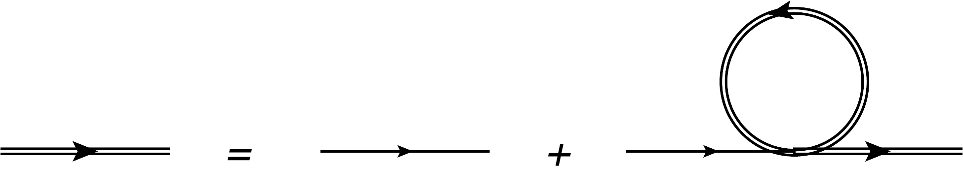
Figure 1. Diagrammatic representation of Eq. (2), which establishes the connection between dressed quark (double solid line) with constituent mass
$ M_f $ and bare quark (single solid line) with current quark mass$ m_f $ .$ \begin{aligned}[b] \Omega = & - {2 N_c N_f} \int {\frac {{\rm d}^3 p} {(2 \pi)^3}}{\sqrt {p^2 + M^2}}\\& - {2 N_c N_f T} \int {\frac {{\rm d}^3 p}{(2 \pi)^3}} \Bigg(\ln\left(1+\exp\left(-\frac{(E-\mu)}{T}\right)\right)\\ & + \ln \left(1+ \exp \left(-\frac{(E+\mu)}{T}\right)\right)\Bigg) + \frac{(M - m)^2}{4G} \end{aligned} $

(3) where each term bears its usual significance, which can be found in [39,40].
Next, to study mesonic states as a quark condensate, the conventional step is to iterate the four-point vertex as presented in Fig. 2, which interprets that infinite series of quark-anti-quark loops are equivalent to a meson propagator [37,38,40,41]. The mesonic polarization function
$ \Pi_{\pi,\sigma} $ is given as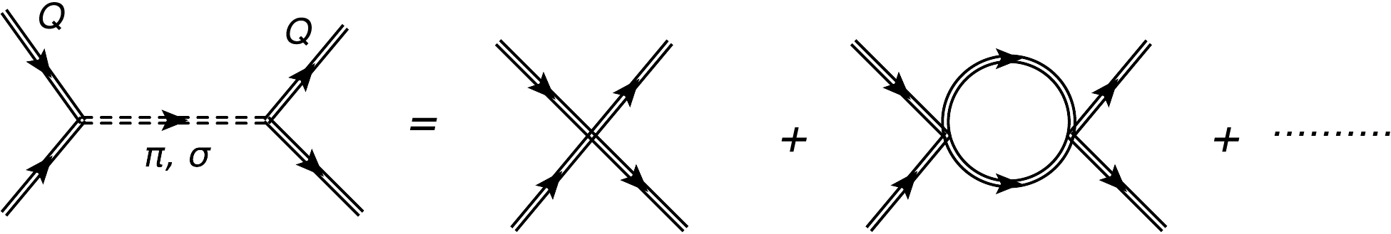
Figure 2. Diagrammatic representation of the transformation of a quark-quark interaction into an effective
$ \pi $ ,$ \sigma $ meson propagators (double dash line).$ \Pi^{M,M^\prime}_{\pi,\sigma} (\omega, \vec{q}) = \int_\lambda {\frac{{\rm d}^4p}{(2\pi)^4}} {\rm Tr} (\gamma_M S(p+q) \gamma_{M^\prime} S(q)) $

(4) where
$ S(p) $ denotes the Hartree quark propagator.$ \gamma_M $ refers to the scalar or pseudoscalar interaction vertex and the index$ M $ denotes the scalar or pseudoscalar interaction channel. The polarization function can be expressed as [40]$ \Pi^{M, M^\prime} = I_1 - (\omega^2 - q^2 -\epsilon^2_{M, M^\prime}) I_2 (\omega, \vec q) $

(5) where
$ I_1 = N_c N_f \int_\lambda {\frac{{\rm d}^3p}{(2\pi)^3}} {\frac{1}{E_p}} \left[\tanh {\frac{\beta(E_p + \mu)}{2}} + \tanh {\frac{\beta (E_{p} - \mu)}{2}} \right] $

(6) and the function
$ I_2(\omega, \vec q) $ given as$ \begin{aligned}[b] I_2 (\omega, \vec q) = & - N_c N_f \int_\lambda {\frac{{\rm d}^3 p}{(2 \pi)^3}} {\frac{1}{2 E_p E_(p+q)}}\\ & \times \Bigg\{ {\frac{1}{\omega + E_p -E_{p+q}}}[n(E_p - \mu) - n(E_{p+q}- \mu) \\ &+ n(-E_{p+q} -\mu) - n(-E_p - \mu)]\\ & + \left[{\frac{1}{\omega-E_p -E_{p+q}}}-{\frac{1}{\omega+E_p +E_{p+q}}}\right]\\ & \times [n(E_p - \mu) - n(-E_{p+q}-\mu)]\Bigg\}. \end{aligned}$

(7) The complex function that appears in the thermodynamic potential can be simplified, as it can be expressed as [40]
$ 1-2G \Pi_M (\omega+{\rm i}\epsilon, \vec q) = [1 - 2G \Pi_M(\omega-{\rm i}\epsilon, \vec q)] \exp(-2{\rm i} \Phi_M (\omega, \vec q)), $

(8) $ \Phi_M $ represents the scattering phase shift associated with the quark-antiquark scattering in the interaction channel and it can be divided in two parts$ \Phi_M = \phi + \phi_M $

(9) with
$ {\rm tan} \phi = -\frac{{\rm Im} I_2 (\omega + {\rm i}\epsilon, \vec q)}{{\rm Re} I_2 (\omega + {\rm i}\epsilon, \vec q)} $

(10) and
$ {\rm tan}\phi_M = -\frac{{\rm Im} M^2(\omega +{\rm i}\epsilon, \vec q)} {(\omega^2 - q^2-\epsilon^2_M + {\rm Re} M^2(\omega+{\rm i}\epsilon, \vec q))} , $

(11) where
$ M^2(\omega,\vec q) = \frac{1-2GI_1}{2GI_2(\omega,\vec q)} , $

(12) where
$ \phi_M $ denotes the meson phase shift and$ \phi $ represents the background phase shift. The mass of the meson is extracted from the pole of the meson propagator in Random Phase Approximation at zero momentum, which is given by the following equation [38,40]$ 1- 2G \,{\rm Re}\, \Pi_{\pi,\sigma} (m_{\pi, \sigma}, \overrightarrow{0}) = 0\; , $

(13) where the real part of
$ \Pi_{\pi, \sigma} (\omega, \vec{0}) $ are expressed as [38]$ {\rm Re}\Pi_\pi (\omega, \vec{0}) = 2 N_c N_f\int\frac{{\rm d}^3p}{(2\pi)^3} \frac{(1-2n_p)}{ \omega_p} \frac{ \omega_p^2}{ \omega_p^2- \omega^2/4} , $

(14) $ {\rm Re}\Pi_\sigma (\omega, \vec{0}) = 2 N_c N_f\int\frac{{\rm d}^3p}{(2\pi)^3} \frac{(1-2n_p)}{ \omega_p} \frac{ \omega_p^2-M_q^2}{ \omega_p^2- \omega^2/4}\, . $

(15) The mass of the unbound resonance has been considered as the real part of
$ \Pi_{\pi, \sigma} $ at zero density. For$ (\omega = m_{\pi, \sigma} < 2M_q) $ , the imaginary part of the polarization function is zero; hence, the decay channel into the dressed$ q \bar q $ pair is closed, and the spectral function gets a bound state contribution expressed by a delta peak in correspondence of the meson mass. For$ m_{\pi, \sigma} > 2M_q $ , the meson can decay into a constituent quark-antiquark pair. Hence, it is not a stable bound state, but a resonant state.$ \Pi_{\pi, \sigma} $ has an imaginary part, and the meson spectral function receives a contribution from the continuum cut. Then, the pole mass equation can be expressed in the complex form to determine the resonant mass$ m_{\pi,\sigma} $ and its associated decay width$ \Gamma_{\pi,\sigma} $ from the relationship [40],$ 1-2G \Pi_{\pi,\sigma}\left(m_{\pi,\sigma}-{\rm i}\frac{1}{2}\Gamma_{\pi,\sigma},\vec 0\right) = 0 $

(16) From the imaginary part of
$ M^2 $ , we can define the decay width as,$ \Gamma_{\pi,\sigma} = \frac{{\rm Im} M^2 (m_{\pi,\sigma}-{\rm i}\epsilon, \vec 0)}{m_{\pi,\sigma}} , $

(17) where [38]
$ \begin{aligned}[b] {\rm{Im}}I_2^\pi (\omega ,\vec 0) =& \theta ({\omega ^2} - 4M_q^2)\theta (4({\Lambda ^2} + M_q^2) - {\omega ^2})\\&\times\frac{{{N_c}{N_f}}}{{16\pi }}{\omega ^2} \sqrt {1 - \frac{{4M_q^2}}{{{\omega ^2}}}} [1 - 2n(\omega /2)]\;, \end{aligned} $

(18) $ \begin{aligned}[b] {\rm Im}I_2^{\sigma}(\omega, \vec {0}) = & \theta (\omega^2 - 4M_q^2)\theta (4(\Lambda^2 +M_q^2)- \omega^2) \\&\times{\frac{N_c N_f}{16\pi}}(\omega^2-4M_q^2) \sqrt{1-\frac{4M_q^2}{ \omega^2}}\\&\times[1-2n( \omega/2)]\; . \end{aligned} $

(19) To implement the effect of finite system sizes, proper boundary conditions must be chosen: periodic for bosons and anti-periodic for fermions. In effect, this leads to a sum of infinite extent over discretized momentum values,
$ p_i = \dfrac{\pi n_i}{R} $ , where$ R $ denotes the dimension of cubical volume and$ n_i $ are positive integers with i = x, y, z. Negative values of$ n_i $ are neglected, because they will provide wave-functions identical to the positive$ n_i $ solutions except for a physically irrelevant sign change. Here, we have done several simplifications: i) We neglect surface and curvature effects. ii) The infinite sum is considered as an integration over a continuous variation of momentum, but with the lower cut-off. iii) We do not adopt any modifications to the mean-field parameters due to finite size effects. Our philosophy had been to maintain the known physics at zero$ T $ , zero$ \mu $ , and infinite volume fixed.This implies a lower momentum cut-off
$p_{\rm min}\approx\dfrac{\pi}{R} = \lambda (\rm say)$ . The infinite sum over discrete momentum values is replaced by integration over continuum momentum variation, but with the lower momentum cut-off. Hence, by replacing the lower limit zero by the lower cut-off$ \lambda $ in Eq. (2), Eqs. (14)–(15), and Eqs. (18)–(19), we obtain modified results of constituent quark mass$ M_q $ , meson masses$ m_{\pi, \sigma} $ , and meson dissociation probabilities$ \gamma_{\pi, \sigma} $ , which depend on the volume of the medium along with the temperature of the medium.In principle, discrete momentum values should be summed over, but for simplicity, we integrate over continuous values of momentum. This simplified picture of the finite size effect by implementing a lower momentum cut-off is well justified in Refs. [42,43]. It is well demonstrated in Fig. 1 of Ref. [42].
-
It is known that
$ \pi $ and$ \sigma $ mesons are pseudo-scalar and scalar modes comprising$ u, d $ quarks with the same spin quantum no ($ J = 0 $ ) but different parity states$ \pi = -1, +1 $ . Particle physicists generally follow the compact notation of the spin and parity quantum number as$ J^\pi $ . Hence, we can visualize that$ \pi $ and$ \sigma $ mesons are$ J^\pi = 0^{-1} $ and$ 0^{+1} $ quantum states of the same quark composition. They are called chiral partners. Quarks are the fundamental building blocks of hadrons, and a non-zero quark condensate is responsible for the mass difference between chiral partners at$ T = 0 $ . Therefore, by increasing the temperature of nuclear or hadronic matter, a phase transition from hadrons to quarks can occur beyond a transition temperature, and the corresponding condensate also melts down. Owing to this transformation from large to nearly zero condensate and breaking to the restoration phase of chiral symmetry, the mass difference between chiral partners disappears. The NJL model (as well as other effective QCD models) can optimally capture these facts, and its mathematical framework has already been addressed in Sec. II.B, while its results will be discussed in Sec. III. In this subsection, we will discuss the drag, diffusion, and conduction of two mesonic modes via dissociations into quarks and anti-quarks. The mathematical anatomy of the dissociation process has already been addressed in Eqs. (18)–(19) and it can be directly connected with drag and then with the diffusion and conduction of chiral partners. Here, we will first devlop the diagrammatic construction of conductivity and diffusion. Then, in the end, we will observe the position of the drag coefficient in the diagrammatic expression of conductivity and diffusion. In real-time thermal field theory, any two point function at finite temperature can always be expressed in a$ 2\times 2 $ matrix structure because the contour in a complex time plane offers four possible sets of two points [44,45]. For a symmetric contour (although there are many other ways to draw it), time evolution starts from$ -\infty $ to$ +\infty $ along a horizontal real-time axis, then it shifts down along the imaginary-time axis by$ -i\frac{\beta}{2} $ , and then returns from$ +\infty $ to$ -\infty $ ; finally, it completes its remaining shift by$ -i\frac{\beta}{2} $ along imaginary-time axis, such that its final destination point is$ -i\beta $ . This time evolution along the imaginary-time axis up to$ -i\beta $ is the basic requirement of thermal field theory, where the time evolution operator has to be converted into a density matrix [44,45]. In real time formalism, we have two real-time axes from$ -\infty $ to$ +\infty $ and from$ +\infty $ to$ -\infty $ . Four possible approaches are available to choose two points on these two axes, which can be considered as four components of a$ 2\times 2 $ matrix structure. Realizing the propagator as a two-point function of field operators, if one can proceed for finding thermal propagator in real-time formalism, then a$ 2\times 2 $ matrix structures with four components$ D^{11} $ ,$ D^{12} $ ,$ D^{21} $ ,$ D^{22} $ can be found. Similarly, one-loop self-energy at finite temperature forms a$ 2\times 2 $ matrix structure with four components$ \Pi^{11} $ ,$ \Pi^{12} $ ,$ \Pi^{21} $ ,$ \Pi^{22} $ .This matrix can normally be diagonalized in terms of a single element like retarded component
$ \Pi^R_{\mu\nu}(q_0, \vec q) $ or the spectral function$ \rho_{\mu\nu}(q_0, \vec q) $ of that mesonic correlator. Starting with 11 components ($ \Pi^{11}_{\mu\nu} $ ) of the$ 2\times 2 $ matrix, anyone of these quantities can be obtained by adopting their connecting relationship [46,47]:$ \begin{aligned}[b] \rho_{\mu\nu}(q_0, \vec q) = &2{\rm Im}\Pi^R_{\mu\nu}(q_0, \vec q) {}\\ = &2{\rm tanh}(\frac{\beta q_0}{2}){\rm Im}\Pi^{11}_{\mu\nu}(q_0, \vec q)\; . \end{aligned} $

(20) Using the Wick contraction technique, 11 components of the current-current correlator can be derived as [46,47]
$ \begin{aligned}[b] \Pi^{11}_{\mu\nu}(q_0, \vec q) = & {\rm i}\int {\rm d}^4x {\rm e}^{{\rm i}qx}\langle T J_\mu(x)J_\nu(0) \rangle_\beta {}\\ = & {\rm i}\int {\rm d}^4x {\rm e}^{{\rm i}qx} \langle T{\phi}\underbrace{(x){\partial}_\mu{\phi}\overbrace{(x) {\phi}}(0){\partial}_\nu\phi}(0)\rangle_\beta {}\\ = & {\rm i}\int \frac{{\rm d}^4k}{(2\pi)^4}N_{\mu\nu}(q,k) D_{11}(k)D_{11}(p = q+k)\; , \end{aligned} $

(21) where
$ D^{11}(k) = \frac{-1}{k_0^2- \omega_k^2+ {\rm i} \epsilon}+2\pi i n_k \delta(k_0^2- \omega_k^2)\; , $

(22) where
$n_k = 1/({\rm e}^{\beta \omega_k} - 1)$ represents Bose-Einstein (BE) distribution function of mesonand
$ N_{\mu\nu}(q,k) = -4k_\mu(q-k)_\nu\; . $

(23) Eq. (21) can diagrammatically be associated with a one-loop type of self-energy diagram with internal meson lines, as illustrated in Fig. 3(A). Then, from this correlator
$ \Pi^{11}_{\mu\nu} $ , it is possible to obtain the useful correlators - (1). The density-density correlator is obtained as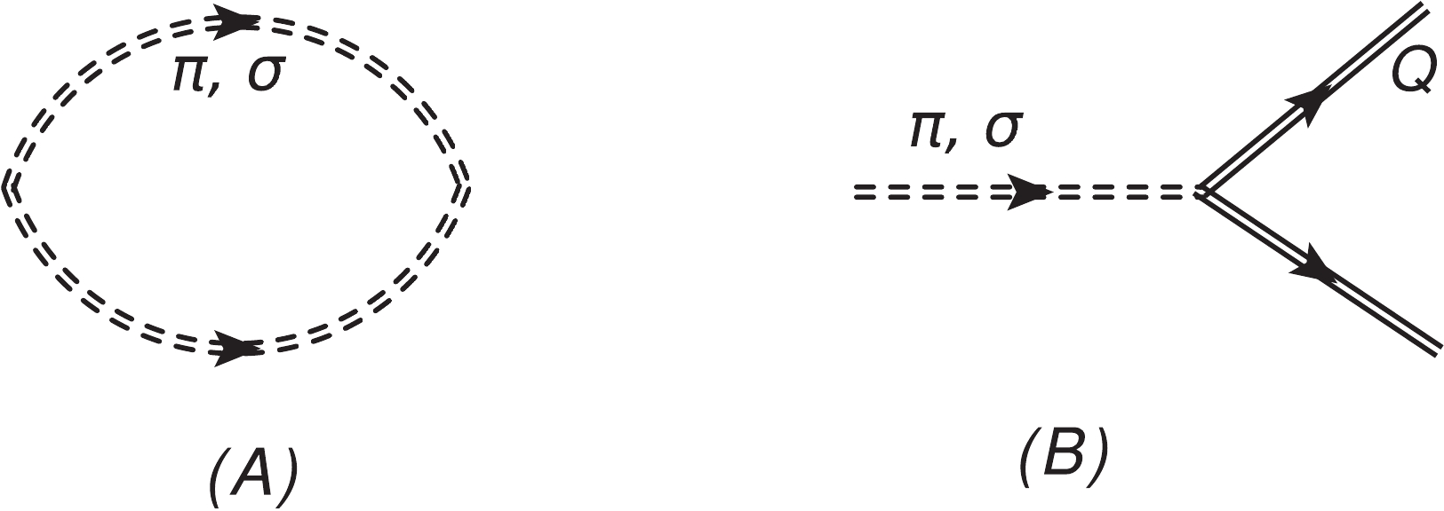
Figure 3. (A) One-loop schematic representation of
$ \pi $ or$ \sigma $ meson current-current correlator, whose low frequency limit is connected with its diffusion coefficient or conductivity. (B) Dissociation diagram of$ \pi $ or$ \sigma $ meson to quark and anti-quark.$ \Pi^{R}_{00}(q_0, \vec q) = {\rm i}\int {\rm d}^4x {\rm e}^{{\rm i}qx}\langle [J_0(x),J_0(0)]\rangle_\beta $

(24) (2), while the spatial current-current correlator is defined as
$ \Pi^{R}_{ij}(q_0, \vec q) = {\rm i}\int {\rm d}^4x {\rm e}^{{\rm i}qx}\langle [J_{i}(x),J_{j}(0)]\rangle_\beta\; . $

(25) The spatial current-current correlator can be decomposed into transverse and longitudinal components as
$ \Pi^{R}_{ij}(q_0, \vec q) = \left(\frac{q_iq_j}{q^2} -\delta_{ij} \right)\Pi^{R}_{T}(q_0, \vec q) + \frac{q_iq_j}{q^2}\Pi^{R}_{L}(q_0, \vec q)\; , $

(26) where our matter of interest is on the longitudinal component
$ \Pi^{R}_{L}(q_0, \vec q) $ , which can be extracted from both density-density and (spatial) current-current correlators by using the relationship$ \Pi^{R}_{L}(q_0, \vec q) = \frac{q_0^2}{q^2}\Pi^{R}_{00}(q_0, \vec q) = \frac{q^iq^j}{q^2}\Pi^{R}_{ij}(q_0, \vec q)\; . $

(27) Hence, we can define a spectral function without Lorentz indices
$ \rho = 2\Pi^{R}_{L}(q_0, \vec q)\; . $

(28) Using Eq. (22) in Eq. (21) and then using the other Eqs. (20), (28), we obtain the simplified structure in a positive but low
$ q_0 $ region [46,47]$ \begin{aligned}[b] \rho(q_0, \vec q) =& 2\int\frac{{\rm d}^3k}{(2\pi)^3} \frac{(-\pi)N}{4 \omega_k \omega_p}\\&\times[q_0\beta\{n^+_k(1-n^+_k)\}\delta(q_0+ \omega_k- \omega_p)] {}\\ =& 2\int\frac{{\rm d}^3k}{(2\pi)^3} \frac{N}{4 \omega_k \omega_p}\lim\limits_{\gamma \rightarrow 0}\left[ \frac{q_0\beta\{n^+_k(1-n^+_k)\}\gamma}{(q_0+ \omega_k- \omega_p)^2+\gamma^2}\right]\; . \end{aligned} $

(29) We will consider the finite value of
$ \gamma $ in further calculations to obtain non-divergent values of pion ($ \pi $ ) and sigma ($ \sigma $ ) meson conductivity$ \begin{aligned}[b] \kappa =& \frac{1}{6}\lim\limits_{q_0, \vec q \rightarrow 0}\frac{\rho(q_0, \vec q)}{q_0} {}\\ = &\frac{1}{\gamma}2\beta\int^{\infty}_{0} \frac{{\rm d}^3 \vec k}{(2\pi)^3}\frac{1}{3}\Big(\frac{ \vec k}{ \omega_k}\Big)^2[n_k\{1+n_k\}] \end{aligned} $

(30) where
$ \chi_s = 2\beta\int^{\infty}_{0} \frac{{\rm d}^3 \vec k}{(2\pi)^3}[n_k\{1+n_k\}] $

(31) represents static susceptibility and
$ \omega_k = \{ \vec k^2+m_{\pi,\sigma}^2\}^{1/2} $ . Therefore, by identifying$ \gamma_{\pi,\sigma} $ as the drag coefficient of$ \pi $ and$ \sigma $ mesons, one can calculate spatial diffusion constant$ D = \kappa/\chi_s $

(32) Eq. (29) can be approximated as
$ \kappa = \frac{1}{\gamma}\langle v^2/3\rangle\chi_s\; , $

(33) and then using the further approximated relationship
$ \langle v^2/3\rangle = T/m $ , based on the non-relativistic equipartition theorem, Einstein relationship can easily be determined$ \langle v^2/3\rangle\frac{1}{\gamma} = \frac{T}{m_{\pi,\sigma}\gamma} = D\; . $

(34) Eqs. (30) to (34) basically represents general connections among the quantities -
$ D $ ,$ \gamma $ ,$ \kappa $ ,$ \chi_s $ . For$ \pi $ and$ \sigma $ mesonic condensates, these quantities can be denoted as$ D_{\pi,\sigma} $ ,$ \gamma_{\pi,\sigma} $ ,$ \kappa_{\pi,\sigma} $ ,$ \chi^{\pi,\sigma}_s $ respectively. Similar calculations of the same quantities for heavy quark can be found in Ref. [48].Here, we want to obtain drag (
$ \gamma_{\pi,\sigma} $ ), diffusion ($ D_{\pi,\sigma} $ ) coefficients, and conductivity ($ \kappa_{\pi,\sigma} $ ) for$ \pi $ and$ \sigma $ mesons near and beyond Mott temperature, where these mesonic condensates can dissociate in quarks and anti-quarks in the medium via the decay process$ \pi/\sigma\rightarrow Q + {\bar Q} $ and the mesonic condensates will dissipate through a medium, whose corresponding$ \gamma_{\pi,\sigma} $ ,$ D_{\pi,\sigma} $ , and$ \kappa_{\pi,\sigma} $ we wish to estimate. Here, drag coefficients of$ \pi,\sigma $ states are estimated via the decay process of$ \pi\rightarrow Q{\bar Q} $ and$ \sigma\rightarrow Q{\bar Q} $ . Hence, we can precisely equate$ \gamma_{\pi,\sigma} $ with Eq. (17), which estimates the decay probability of$ \pi, \sigma\rightarrow Q{\bar Q} $ from the imaginary part of the mesonic self-energy. These dissociation diagrams are illustrated in Fig. 3(B). After obtaining the drag coefficients$ \gamma_{\pi,\sigma} $ , we can calculate$ D_{\pi,\sigma} $ and$ \kappa_{\pi,\sigma} $ using Eqs. (30), (32). -
This section will numerically explore the spectral and dissipation properties of chiral partners
$ \pi $ and$ \sigma $ mesons at finite temperature and size. Their masses will reveal their spectral properties, while their drag, diffusion, and conductivity will measure their dissipation properties.The masses of the
$ \pi $ and$ \sigma $ mesons are obtained from Eqs. (13)–(15), and the decay widths can be calculated from Eqs. (17)–(19). Fig. 4 presents the temperature dependence of chiral partners,$ \pi $ and$ \sigma $ mesons, for different system sizes$ R $ . In real world (for$ T = 0 $ ), their masses are well separated; however, they will be in degenerate states at a high temperature. This fact of merging chiral partners is considered as an alternative signature of chiral symmetry restoration. This transition from chiral symmetry breaking to restoration is observed for both infinite and finite system sizes; however, their merging pattern becomes different. In the beginning, pion mass increases and sigma meson mass decreases with$ T $ , then beyond the transition temperature, both increase to be merged. In this context, the reader may find an interesting trend pion mass in Ref. [49], where it can be reduced near the transition temperature. At$ T = 0 $ , the mass of the$ \pi $ meson increases as we decrease the system size, while the mass of$ \sigma $ meson remains unchanged. As the volume decreases, the difference between$ \pi $ and$ \sigma $ mesons also decreases, which indicates that the chiral symmetry effect reduces with decreasing volume. The exact mathematical analysis finite volume effect on Eqs. (14) and (15) might be a challenging job; however, shrinking the thermodynamical phase-space can be considered as the main source of modifications. Results obtained from the increasing pion mass with decreasing volume have also been observed in other frameworks like the chiral perturbation theory [50] and renormalization group methods in the quark-meson model [51]. However, the pion mass generally shoots up after the critical temperature in the infinite volume case, but its blowing trend becomes quite suppressed in the finite volume case. As collective result of increasing the pion mass and suppressing blowing trends after critical temperature, we infer that the masses are suppressed from$ R = \infty $ to$ R = 4\; \rm{fm} $ , whereas they are enhanced from$ R = 4\; \rm{fm} $ to$ R = 2\; \rm{fm} $ .
Figure 4. (color online)
$ T $ dependence of pion (black) and sigma (red) meson masses for$ R=\infty $ (solid line),$ 4 $ fm (dash-dotted line),$ 3 $ fm (dash line), and$ 2 $ fm (dotted line).Next, in Fig. 5, we have plotted
$ \pi $ and$ \sigma $ decay widths in a$ Q{\bar Q} $ channel for different system sizes. Because the$ \sigma $ meson mass is more significant than two times the quark mass ($ m_\sigma>2M_q $ ) in the entire temperature range, we will obtain non-zero$ \gamma_\sigma $ in the entire$ T $ . However, for the case of the$ \pi $ meson mass, the kinematic threshold$ m_\pi>2M_q $ is valid above the Mott temperature$ T_M $ , below which the$ \pi\rightarrow Q{\bar Q} $ decay is forbidden. For$ R = \infty $ case,$ T_M = 0.201 $ GeV, and it shows that the solid black line, denoting$ \gamma_\pi $ , is non-zero beyond that temperature. In this study, we have only considered the dissociation diagram of pion. This explains why we obtain this kind of pattern. However, one can obtain a non-zero scattering probability of pion below the Mott temperature$ T_M $ by considering other possible scattering diagrams. For example,$ \pi + \pi \rightarrow \pi + \pi $ scattering is possible in higher-order diagrams as addressed in Ref. [52]. Accordingly, this present study is intended to solely consider the dissociation diagram and zoom in on the finite size effect of merging patterns of chiral partners. A merging pattern in the decay width of chiral partners is observed. It is expected that as the kinematic phase-space of two decay probabilities depend on their mass only, their coupling constants are not different, and similar to the NJL model,$ \pi $ and$ \sigma $ meson states are basically considered as condensates of the same quark composition, but with a different spin-parity quantum number$ J^\pi $ (=$ 0^- $ and$ 0^+ $ for$ \pi $ and$ \sigma $ meson respectively). When we consider the finite size effect, we find that the$ \gamma_\sigma $ increases in the low$ T $ domain. Mott temperature decreases as$ R $ decreases, which can be observed from shifting the threshold pion decay width along the$ T $ -axis.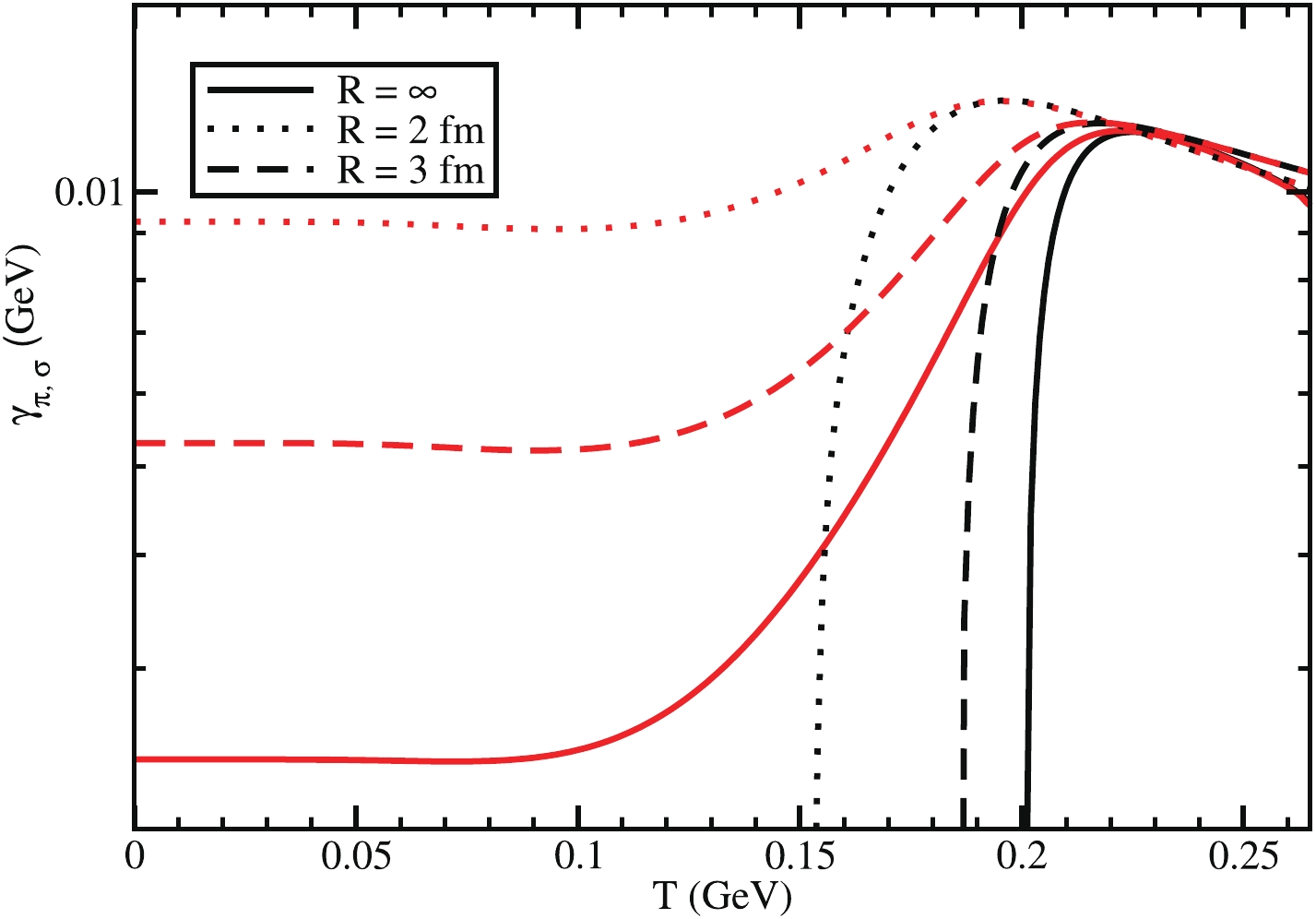
Figure 5. (color online)
$ T $ dependence of pion (black) and sigma (red) meson decay widths through quark-anti-quark channel for different system sizes.Fig. 6(a) presents quark masses as a function of
$ T $ and$ R $ . It can be observed that$ M_q $ decreases with decreasing system size due to the shrinking of the phase-space integration in gap Eq. (2). Accordingly, due to the term$ \sqrt{m_{\pi,\sigma}-4M_q^2} $ in Eqs. (18) and (19), the$ \gamma_{\pi, \sigma} $ become larger (in low T domain) as the system size decreases. Knowing$ M_q(T,R) $ and$ m_\pi(T,R) $ , the Mott temperature$ T_M(R) $ can be determined as a function of$ R $ , where$ m_\pi-2M_q = 0 $ . It is plotted in Fig. 6(b), from where we obtain$ T_M(R) $ , which is plotted as a solid red line with circles in Fig. 7. From Fig. 6 it can be observed that the Mott temperature value decreases in a lower system size. The value of the Mott temperature for$ R = 2 $ fm is quite smaller than the higher volume systems.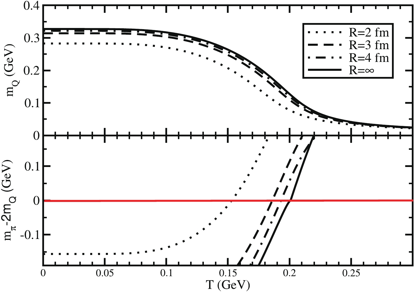
Figure 6. (color online)
$ T $ dependence of (a)$ M_q $ and (b)$ m_\pi-2M_q $ for different system sized. Straight horizontal red lined, located at$ m_\pi-2M_q = 0 $ , are indicating corresponding Mott temperature$ T_M $ for different values of$ R $ .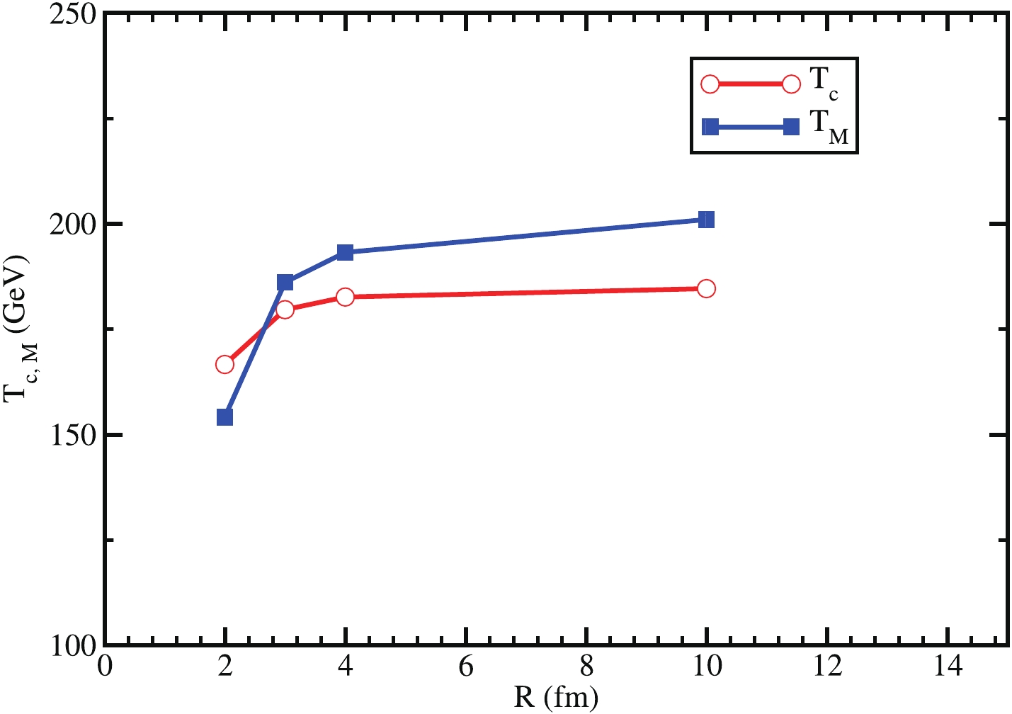
Figure 7. (color online) Modification of transition temperature
$ T_c $ and Mott temperature$ T_M $ for changing the system size$ R $ , where$ R = 10 $ is approximately considered as infinite volume.Fig. 7 represents the variation of the transition temperature and Mott transition temperature with
$ R $ . The transition temperature can be obtained from the maxima of the first derivative of the chiral condensates for the different finite system sizes. As$ R $ increases, both the transition and Mott transition temperatures increase, and after$R = 4\; {\rm fm}$ , they both attain saturation. The value of the Mott transition temperature is lower than that of the transition temperature below$R = 3\; {\rm fm}$ . As we increase the system's size, the Mott temperature value starts increasing more than the transition temperature and saturates at a higher value than the transition temperature.Using the
$ m_{\pi,\sigma}(T,R) $ and$ \gamma_{\pi,\sigma}(T,R) $ in Eq. (30), we have obtained the conductivity of the pion and sigma$ \kappa_{\pi,\sigma}(T,R) $ , which is plotted in Fig. 8. Below the Mott temperature, a divergence trend and sharp divergence of$ \kappa_{\pi}(T,R) $ are observed for infinite and finite system size cases. The source of divergence is the relationship$ \kappa_{\pi}\propto 1/\gamma_{\pi} $ . The pion and sigma meson's conductivity changes significantly with the variation of the system size and decreases with the decreasing volume. The conductivity of the pion and sigma meson merges after the transition temperature, which is again decreased as the system size decreases.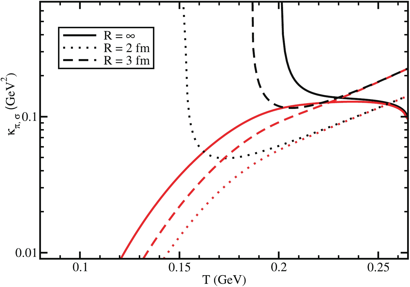
Figure 8. (color online) Conductivity of
$ \pi $ (black) and$ \sigma $ (red) mesons or light flavor condensates with quantum numbers$ J^\pi=0^- $ and$ 0^+ $ for$ R=\infty $ (solid line) and$ 2 $ fm (dotted line).Fig. 9(a) shows the diffusion coefficients of
$ \pi $ and$ \sigma $ mesons by using Eq. (32), while Fig. 9(b) shows corresponding results by using the Einstein relationship given in Eq. (34). Furthermore, one can notice the divergence nature of$ D_{\pi}(T,R) $ below the Mott temperature and realize the feasible relationship$ D_{\pi}\propto 1/\gamma_\pi $ .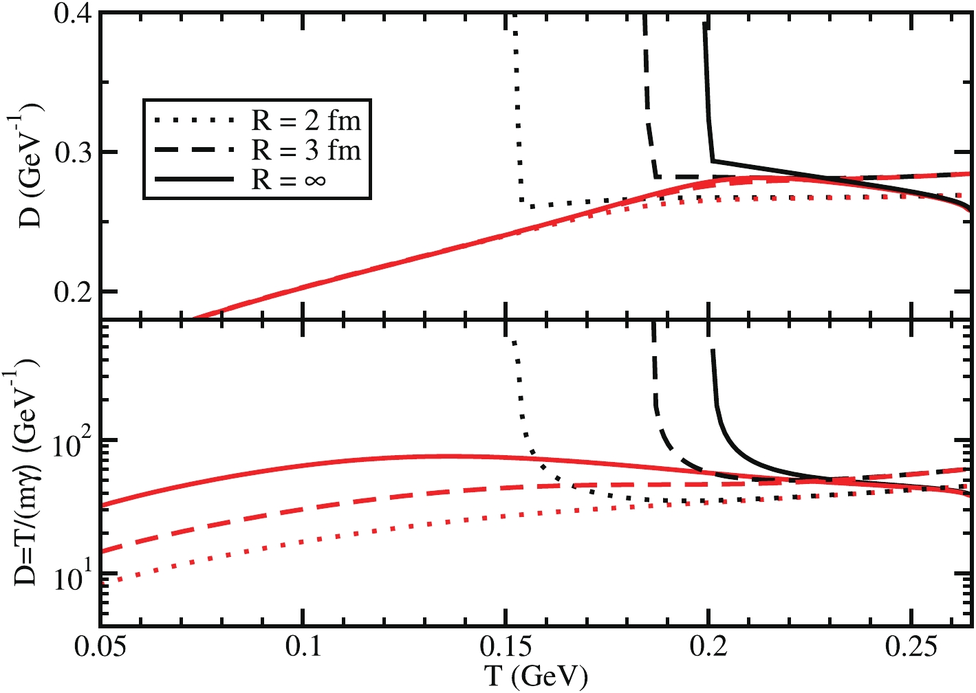
Figure 9. (color online) Diffusion coefficients
$ D $ of$ \pi $ (black) and$ \sigma $ (red) mesons or light flavor condensates with quantum number$ J^\pi = 0^- $ and$ 0^+ $ for$ R = \infty $ (solid line),$ 3 $ fm (dash line), and$ 2 $ fm (dotted line).At the end, if we briefly take a look at all the quantities of chiral partners for infinite (
$ R = \infty $ ) and finite ($ R = 2 $ fm) sizes of the medium, we can obtain a table, as presented in Table 1. The transition and Mott temperatures for$ R = \infty $ and$ R = 2 $ fm are presented in Table 1, which also includes the temperatures, where the masses ($4^{\rm th}$ column), drag coefficients ($2^{\rm nd}$ column), diffusion coefficients ($3^{\rm rd}$ column), and conductivity ($4^{\rm th}$ column) of$ \pi $ and$ \sigma $ mesons tend to merge. Along with the well-known conventional concepts of transition and Mott temperatures, we have defined the temperatures, beyond which the system forms the doublet of masses, drag coefficients, diffusion coefficients, conductivity. All these temperatures reveal a common fact that their positions shift towards lower values during the transition from infinite to finite system sizes. Similar to chiral condensate melting, forming mass doublets beyond the transition temperature is another demonstration of chiral symmetry restoration. Accordingly, merging other quantities such as drag, diffusion coefficients, and conductivity might also be considered alternative realization chiral symmetry restoration. In fact, collecting all quantities provides a deep understanding of the different thermodynamical properties of chiral partners and transition details from breaking to restore the phase of chiral symmetry. The transition point with respect to the drag, diffusion coefficients, and conductivity will also shifts in a lower temperature when one goes from infinite to finite size matter.Size Transition
TemperatureMott
TemperatureMass
Doublet$ R=\infty $ 

184 200 245 $ R=2 $ fm

166 153 223 Size Drag
DoubletDiffusion
DoubletConductivity
Doublet$ R=\infty $ 

234 245 236 $ R=2 $ fm

188 195 212 Table 1. Transition (
$2^{\rm nd}$ column) and Mott ($3^{\rm rd}$ column) temperatures, where masses ($4^{\rm th}$ column), drag coefficients ($2^{\rm nd}$ column), diffusion coefficients ($3^{\rm rd}$ column), and conductivity ($4^{\rm th}$ column) of chiral partners are merged for$ R=\infty $ ($2^{\rm nd}$ and$5^{\rm th}$ rows) and$ R=2 $ fm ($3^{\rm rd}$ and$6^{\rm th}$ rows), temperatures are in MeV.At the end, the reader should accept the quantitative limitations of the present simplified approach, where integration with lower momentum cut-off
$ \lambda $ is considered in place of a quantized momentum sum. For a small system with$ R = 2 $ fm, the phase space becomes significantly smaller due to larger values of lower momentum cut-off$ \lambda $ . We observed significant changes in different quantities due to this phase-space shrinking at$ R = 2 $ fm. For this significantly smaller-size case, in principle, we should use quantized momentum sum instead of integration because of larger energy level steps. Again, in place of cubical size, considering the exact cylindrical size of RHIC or LHC matter might be a more realistic problem for phenomenological purposes. All these realistic complicated pictures are not covered in this present study, but will certainly be interesting future research problems. -
We studied the finite volume effect on the spectral functions of strongly interacting matter at zero chemical potential. We presented the pion and sigma meson masses and decay widths at different finite system sizes. In addition, we calculated the conductivity and diffusion coefficients of pion and sigma mesons. All these quantities exhibit significant variations with the finite system size.
At low temperatures, the chiral symmetry is broken, and after the transition temperature, the chiral symmetry is restored. The transition from the chiral symmetry broken phase to the chiral symmetry restored phase can be visualized in both the infinite and finite volume systems. Based on the quark condensate or quark mass melting, we can define a chiral transition temperature, which shifts to lower values when we go from infinite to finite size matter. An alternative chiral symmetry restoration can be realized from the merging of
$ \pi $ and$ \sigma $ masses near and after the transition temperature. This merging point also shifts towards lower temperature due to finite size consideration.We have shown the decay widths of the pion and sigma meson masses with different system sizes. Decay widths are estimated from the imaginary part of self-energy for pion and sigma meson, which interpret the thermodynamical probabilities of their dissociation to quark and anti-quark channels. For the sigma meson, the decay width is observed for the entire temperature range. However, for the pion, the decay width begins after the Mott transition temperature, which also decreases with decreasing system size. Similar to masses of the chiral partners, their decay widths also merge in the temperature domain of the restored phase. Again, the finite size consideration makes their merging points shift towards lower temperature values. For the finite size effect, we find that the decay width of the
$ \sigma $ meson is enhanced in the low$ T $ domain, which is a quite interesting and new outcome.Considering the dissociation process as the dragging mechanism of
$ \pi $ and$ \sigma $ modes with a medium, we estimated their diffusion coefficients and conductivities. Low temperature$ \pi $ mode diffusion or conduction diverges because of the vanishing drag process below the Mott temperature; however, its non-divergent values beyond Mott temperature are merged later with corresponding quantities of$ \sigma $ . Similar to merging the masses and decay widths of chiral partners, their merging of diffusion and conduction values can be considered as an alternative realization of the restored phase, and again, their merging points shift towards the low-temperature direction when the size of the matter is reduced.The finite size effect of quark and hadronic matter, explored in this study, can be connected with RHIC or LHC phenomenology. Here, we have found mass reductions of a constituent quark and pion; however, the mass of the sigma meson remains approximately the same in the low-temperature zone. These changes modify the kinematic phase-space part of meson to quark-antiquark dissociation, as well as the diffusion probabilities of mesons. This finite size effect of the NJL model's phase-space structure can be implemented in other quantities connected with RHIC or LHC phenomenology. For example, in the exploration of the finite size effect on dilepton production, heavy mesons suppression, for which a systematic detail evolution picture has to be adopted. In a finite size system, there is the possibility of a coordinate-dependent condensate, which would be the research topic of a future study.
Finite size effect on dissociation and diffusion of chiral partners in Nambu-Jona-Lasinio model
- Received Date: 2021-05-11
- Available Online: 2022-04-15
Abstract: The masses of pion and sigma meson modes, along with their dissociation in the quark medium, provide detailed spectral structures of the chiral partners. Collectivity has been observed in pA and pp systems both at LHC and RHIC. In this research, we studied the restoration of chiral symmetry by investigating the finite size effect on the detailed structure of chiral partners in the framework of the Nambu-Jona-Lasinio model. Their diffusion and conduction have been studied using this dissociation mechanism. It is determined that the masses, widths, diffusion coefficients, and conductivities of chiral partners merge at different temperatures in the restoration phase of chiral symmetry. However, merging points are shifted to lower temperatures when finite size effect is introduced into the picture. The strengths of diffusions and conductions are also reduced once the finite size is introduced in the calculations.


 DownLoad: