


 Abstract
 HTML
HTML Reference
 Related
 PDF
PDF


-
With over 20 years of development, gauge/gravity duality has become a useful tool to deal with the QCD problem through gravitational theory. Quark-antiquark potential is one of the hottest topics in holographic QCD because heavy quarkonia are among the most sensitive probes used in the experimental study of quark-gluon plasma (QGP) and its properties. The holographic potential of the quark-antiquark pair was first recorded in Ref. [1]. It was found that the quark-antiquark potential exhibits a purely Coulombian (non-confining) behavior and agrees with a conformal gauge theory. Soon after, the potential at finite temperature was discussed in [2, 3]. The deformed
$ AdS_5 $ model and Einstein-Maxwell-Dilation models were used to calculate the quark-antiquark potential in these studies [4–27].Moreover, the recent discovery of a doubly charmed baryon (DHB)
$ \Xi_{c c}+ $ through LHCb experiments at CERN [28, 29] has reinforced interest in the search for a theoretical description of doubly heavy baryons. Inside a DHB, there is a heavy diquark and light quark. Because the heavy quark in a DHB is almost near its mass shell, it is reasonable to expect the heavy quark limit to be applicable in this system [30]. Although lattice gauge theory remains a basic tool for studying nonperturbative phenomena in QCD, it has achieved limited results on QQq potentials to date [31, 32].In recent years, the multi-quark potential from the holographic model has been discussed by Oleg Andreev in Refs. [33–37]. In this effective string model, heavy quarks are connected by string to a baryon vertex, whose action is given by a five brane wrapped around an internal space, and a light quark is a tachyon field coupled to the worldsheet boundary. The main reason for pursuing this model is that its results on the quark-antiquark and three-quark potentials are consistent with lattice calculations and QCD phenomenology [4, 33–37]. The technology we use to extract the QQq potential is same as that in lattice QCD [38]. The QQq potential is extracted from the expectation value of the QQq Wilson loop
$ { W_{QQq}}(R, T) $ . The QQq Wilson loop is constructed from the heavy-quark trajectories and light-quark propagator. Hence, we investigate the QQq potential at finite temperature in this paper using gauge/gravity duality.The remainder of this paper is organized as follows: We establish the different configurations of string at finite temperature in Sec. II. Then, we numerically solve these configurations at different temperatures and provide a discussion in Sec. III. In Sec. IV, we discuss string breaking for the confined phase. Finally, the summary and conclusion are given in Sec. V.
-
First, we briefly review the holographic model used in the paper. Following Ref. [35], this background metric at finite temperature is
$ {\rm d} {\boldsymbol{s}}^{2}={\rm{e}}^{s r^{2}} \frac{R^{2}}{r^{2}}\left(f(r){\rm d} t^{2}+{\rm d} \vec{x}^{\,2}+ f^{-1}(r) {\rm d} r^{2}\right)+{\rm{e}}^{-s r^{2}} g_{a b}^{(5)} {\rm d} \omega^{a} {\rm d} \omega^{b}. $

(1) This model parameterized by s is a one-parameter deformation of Euclidean
$ AdS_5 $ space with a constant radius R, and a five-dimensional compact space (sphere)$ {\boldsymbol{X}} $ , whose coordinates are$ \omega^a $ and$ f(r) $ , is a blackening factor. The Nambu-Goto action of a string is expressed as$ S=\frac{1}{2 \pi \alpha^{\prime}} \int_{0}^{1} {\rm d} \sigma \int_{0}^{T} {\rm d} \tau \sqrt{\gamma}, $

(2) where γ is an induced metric on the string world-sheet (with a Euclidean signature). For
$ AdS_5 $ space,$ f(r) = 1- {r^4}/{r_h^4} $ with the boundary conditions$ f(0) = 1 $ and$ f(r_h) = 0 $ .$ r_h $ is the position of the black hole (brane). The Hawking temperature identified with the temperature of a dual gauge theory can be defined as$ T=({1}/{4 \pi})\left|\partial_{r} f\right|_{r=r_{h}} $ . The motivations for this metric have been clarified in Ref. [35]. However, such a deformed$ AdS_5 $ metric leads to linear Regge-like spectra for mesons [39, 40] and the Cornell potential of a quark-antiquark [4]. The deformed metric satisfies the thermodynamics of lattice [41].Subsequently, we introduce the baryon vertex. According to the AdS/CFT correspondence, this is a five brane [42]. At leading order in
$ \alpha' $ , the brane action is$ S_{\rm vert} = {\cal{T}}_5 \times \int {\rm d}^6 \xi \sqrt{\gamma^{(6)}} $ , where$ {\cal{T}}_5 $ is the brane tension, and$ \xi^{i} $ are the world-volume coordinates. Because the brane is wrapped around the internal space, it appears point-like in$ AdS_5 $ . We choose a static gauge$ \xi^0 = t $ and$ \xi^a = \theta^a $ with$ \theta^a $ coordinates on$ {\boldsymbol{X}} $ . Thus, the action is$ S_{\rm{vert}}=\tau_{v} \int {\rm d} t \frac{{\rm{e}}^{-2 s r^{2}}}{r} \sqrt{f(r)}, $

(3) where
$ \tau_{v} $ is a dimensionless parameter defined by$ \tau_{v}= {\cal{T}}_{5} R {\rm{vol}}({\boldsymbol{X}}) $ , and$ {\rm{vol}}({\boldsymbol{X}}) $ is a volume of$ {\boldsymbol{X}} $ .Finally, we consider that the light quark at string endpoints is a tachyon field, which couples to the world-sheet boundary via
$ S_{q}=\int {\rm d} \tau e \;{T} $ ; this is the usual sigma-model action for a string propagating in the tachyon background [43]. The integral is over a world-sheet boundary parameterized by τ, and e is a boundary metric. We consider a constant background$ {T}(x,r) = {T}_0 $ and worldsheets whose boundaries are lines in the t direction. Thus, the action can be written as$ S_{q}={m} \int {\rm d} t \frac{{\rm{e}}^{\frac{s}{2} r^{2}}}{r} \sqrt{f(r)}, $

(4) where
$ {\rm{m}}=R \;{T}_{0} $ . This is the action of a point particle of mass$ T_0 $ at rest. We choose the model parameters as follows:$ {\boldsymbol{g}}=\dfrac{R^{2}}{2 \pi \alpha^{\prime}}, \;{k}=\dfrac{\tau_{v}}{3 {\boldsymbol{g}}} $ , and$ {n}=\dfrac{m}{\boldsymbol{g}} $ . -
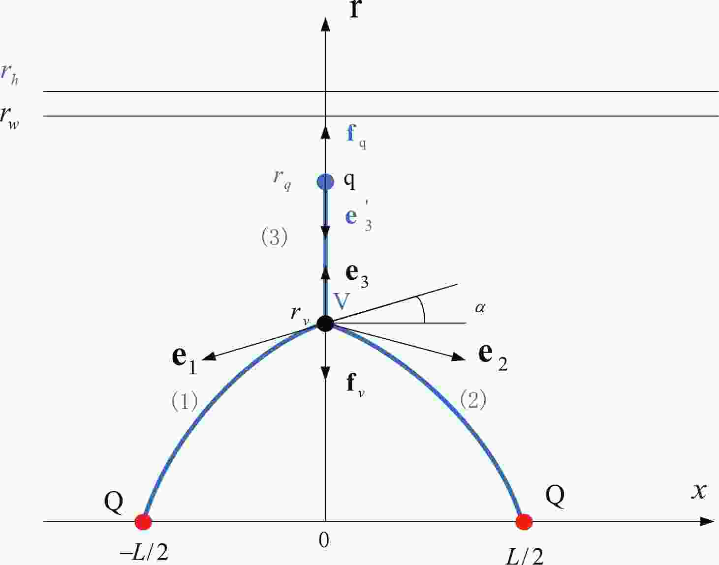
The configuration of QQq is plotted in Fig. 1. The total action is the sum of the Nambu-Goto actions plus the actions for the vertex and background scalar.
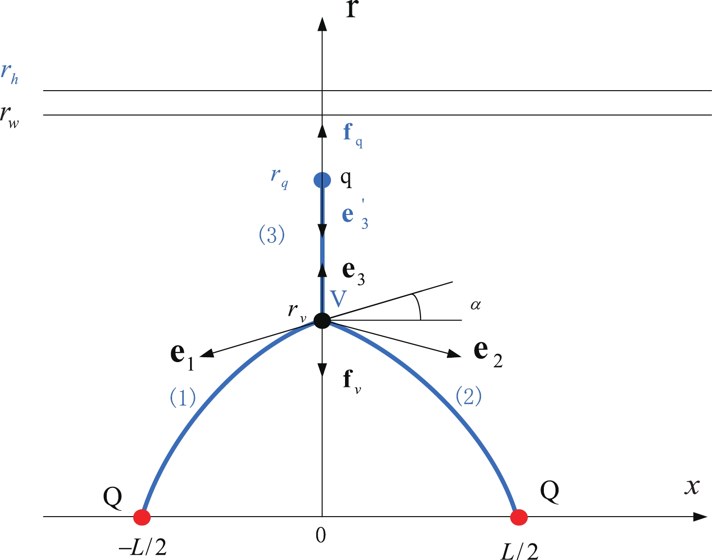
Figure 1. (color online) Static string configuration at a small separation distance of a heavy-quark pair. The heavy quarks Q are placed on the x-axis, while the light quark q and baryon vertex V are on the r-axis at
$r = r_q$ and$r = r_v$ , respectively. The quarks and baryon vertex are connected by the blue string. The force exerted on the vertex and light quark are depicted by the black arrows.$r_h$ is the position of the black-hole horizon.$r_w$ is the position of a soft wall in the confined phase.$ S=\sum\limits_{i=1}^{3} S_{{\rm{NG}}}^{(i)}+S_{\rm{vert}}+S_{q}. $

(5) If we choose the static gauge
$ \xi^{1}=t $ and$ \xi^{2}=r $ , the boundary conditions for$ x(r) $ become$ x^{(1)}(0)=-\frac{L}{2} , \quad x^{(2)}(0)=\frac{L}{2}, \quad x^{(i)}\left(r_{v}\right)=x^{(3)}\left(r_{q}\right)=0. $

(6) The action can now be written as
$ \begin{aligned}[b] S=&{\boldsymbol{g}} T \Bigg(2 \int_{0}^{r_{v}} \frac{{\rm d} r}{r^{2}} {\rm{e}}^{s r^{2}} \sqrt{1+f(r)\left(\partial_{r} x\right)^{2}}\\& +\int_{r_{v}}^{r_{q}} \frac{{\rm d} r}{r^{2}} {\rm{e}}^{{s} r^{2}} \sqrt{1+f(r)\left(\partial_{r} x\right)^{2}}\\&+3 {k} \frac{{\rm{e}}^{-2 {s} r_{v}^{2}}}{r_{v}}\sqrt{f(r_v)} +{n} \frac{{\rm{e}}^{\frac{1}{2} {s} r_{q}^{2}}}{r_{q}}\sqrt{f(r_q)}\Bigg), \end{aligned} $

(7) where
$ \partial_{r} x={\partial x}/{\partial r} $ and$ T=\int_{0}^{T} {\rm d} t $ . We consider the first term in (7), which corresponds to string (1) and (2) in Fig. 1. The equation of motion (EoM) for$ x(r) $ can be obtained from the Euler-Lagrange equation. Thus, we have$ {\cal{I}}=\frac{w(r) f(r) \partial_{r} x}{\sqrt{1+f(r)\left(\partial_{r} x\right)^{2}}}, \quad w(r)=\frac{{\rm{e}}^{{\rm{s}} r^{2}}}{r^{2}}. $

(8) $ {\cal{I}} $ is a constant. At$ r_v $ , we have$ \left.\partial_{r} x\right|_{r=r_{v}}=\cot \alpha $ with$ \alpha>0 $ and$ {\cal{I}}=\frac{w(r_v) f(r_v) {\rm cot} \alpha}{\sqrt{1+f(r)\left({\rm cot} \alpha\right)^{2}}}. $

(9) $ \partial_{r} x $ can be solved as$ \partial_{r} x = \sqrt{\frac{\omega\left(r_{v}\right)^{2} f\left(r_{v}\right)^{2}}{\left(f\left(r_{\nu}\right)+\tan ^{2} \alpha\right) \omega(r)^{2} f(r)^{2}-f(r) w\left(r_{v}\right)^{2} f(r_v)^{2}}}. $

(10) Using (10), the integral over [
$ 0,r_v $ ] of dr is$ L=2 \int_{0}^{r_{v}} \frac{{\rm d}x}{{\rm d}r} {\rm d}r. $

(11) L is a function of
$ r_v $ , α, and$ r_h $ (or equally, temperature). The energy of string (1) can be found from the first term of (7).$ E_R=\frac{S}{T}={\boldsymbol{g}} \int_{0}^{r_{v}}\frac{{\rm d} r}{r^{2}} {\rm{e}}^{{\bf{s}} r^{2}} \sqrt{1+f(r)\left(\partial_{r} x\right)^{2}}. $

(12) Subtracting the divergent term
$ {\boldsymbol{g}} \int_{0}^{\infty}{\rm d}r\dfrac{1}{r^2} $ , we have the regularized energy:$ E_{1}=\frac{S}{T}={\boldsymbol{g}} \int_{0}^{r_{v}}\left(\frac{1}{r^{2}} {\rm{e}}^{{\bf{s}} r^{2}} \sqrt{1+f(r)\left(\partial_{r} x\right)^{2}}-\frac{1}{r^2}\right){\rm d} r - \frac{{\boldsymbol{g}}}{r_v} + c. $

(13) Here, c is a normalization constant. Because string (2) produces the same results, we move to string (3), whose action is given by the second term in (7). This string is a straight string stretched between the vertex and light. The energy can be calculated as
$ E_{2}={\boldsymbol{g}} \int_{r_{v}}^{r_{q}} \frac{{\rm d} r}{r^{2}} {\rm{e}}^{{\rm{s}} r^{2}}. $

(14) Now, we can present the energy of the configuration. From (7), it follows that
$ \begin{aligned}[b] E_{Q Qq} =& {\boldsymbol{g}} \Bigg(2\int_{0}^{r_{v}}\left(\frac{1}{r^{2}} {\rm{e}}^{{\boldsymbol{s}} r^{2}} \sqrt{1+f(r)\left(\partial_{r} x\right)^{2}}-\frac{1}{r^2}\right){\rm d} r\\& - \frac{2}{r_v} + \int_{r_{v}}^{r_{q}} \frac{{\rm d} r}{r^{2}} {\rm{e}}^{{s} r^{2}}+ {n} \frac{{\rm{e}}^{\frac{1}{2} s r_q^2}}{r_q}\sqrt{f(r_q)}\\& +3 {k} \frac{{\rm{e}}^{-2 s r_v^2}}{r_v}\sqrt{f(r_q)}\Bigg) +2 c. \end{aligned} $

(15) The energy is also a function of
$ r_v $ , α, and$ r_h $ . There are two steps to be compeleted: The first is to determine the position of the light quark, which is a function of temperature, and the second is to determine α. To achieve this goal, the net forces exerted on the light quark and vertex vanish. We first write the force balance equation of the light quark as$ {\boldsymbol{f}}_{q}+{\boldsymbol{e}}_{3}^{\prime}=0. $

(16) By varying the action with respect to
$ r_q $ , it is found that${\boldsymbol{f}}_{q}=\left(0,-{\boldsymbol{g}} n \partial_{r_{q}} \left(\big({{\rm{e}}^{\frac{1}{2} {sr}_{q}^{2}}}/{r_{q}}\big)\sqrt{f(r_q)}\right)\right)$ and$ {\boldsymbol{e}}_{3}^{\prime}={\boldsymbol{g}} w\left(r_{q}\right)(0,-1) $ . Hence, the force balance equation becomes$ 2{\rm e}^{({r_q^{2} s})/{2}}\sqrt{f(r_q)}+2n\left(-1+r_q^{2} s\right) f(r_q)+n r_q f^{\prime}(r_q)= 0. $

(17) Note that
$ r_q $ (the position of the light quark) is only a function of$ r_h $ . At fixed temperature,$ r_q $ can be fixed via the above equation. The force balance equation on the vertex is$ {\boldsymbol{e}}_{1}+{\boldsymbol{e}}_{2}+{\boldsymbol{e}}_{3}+{\boldsymbol{f}}_{v}=0. $

(18) $ {\boldsymbol{e}}_{i} $ is the string tension, which can be calculated in the same manner as in Ref. [37]. As a result, the force on the vertex is$ {\boldsymbol{f}}_{v}=\left(0,-3 {\boldsymbol{g}} k \partial_{r_{v}} \left(\big({{\rm{e}}^{-2 s r_{v}^{2}}}/{r_{v}}\big)\sqrt{f(r_v)}\right)\right) $ , and the string tensions are$\begin{aligned}[b]&{\boldsymbol{e}}_{1}={\boldsymbol{g}} w\left(r_{v}\right)\left(-\frac{f(r_{v})}{\sqrt{{\rm tan}^2 \alpha + f(r_{v})}},-\frac{1}{\sqrt{f(r_{v}) {\rm cot}^2 \alpha + 1}}\right), \\&{\boldsymbol{e}}_{2} ={\boldsymbol{g}} w\left(r_{v}\right)\left(\frac{f(r_{v})}{\sqrt{{\rm tan}^2 \alpha + f(r_{v})}},-\frac{1}{\sqrt{f(r_{v}) {\rm cot}^2 \alpha + 1}}\right),\\& {\boldsymbol{e}}_{3}={\boldsymbol{g}} w\left(r_{v}\right)(0,1).\end{aligned}$

The non-trivial component of the force balance equation is
$\begin{aligned}[b]& 2 {\rm e}^{3 s r_v^{2}}\left(1-\frac{2}{1+{\rm cot}\alpha^2 f(r_v)}\right)+6\left(k+4 k s r_v^{2} \right)\sqrt{f(r_{v})}\\-&\frac{3 k r_v f^{\prime}(r_v)}{\sqrt{f(r_v)}}=0. \end{aligned}$

(19) This equation provides the relationship between
$ r_v $ and α when the temperature is fixed. With (15) and (17), we can numerically solve the energy at small L. -
The total action in the configuration plotted in Fig. 2 is expressed as
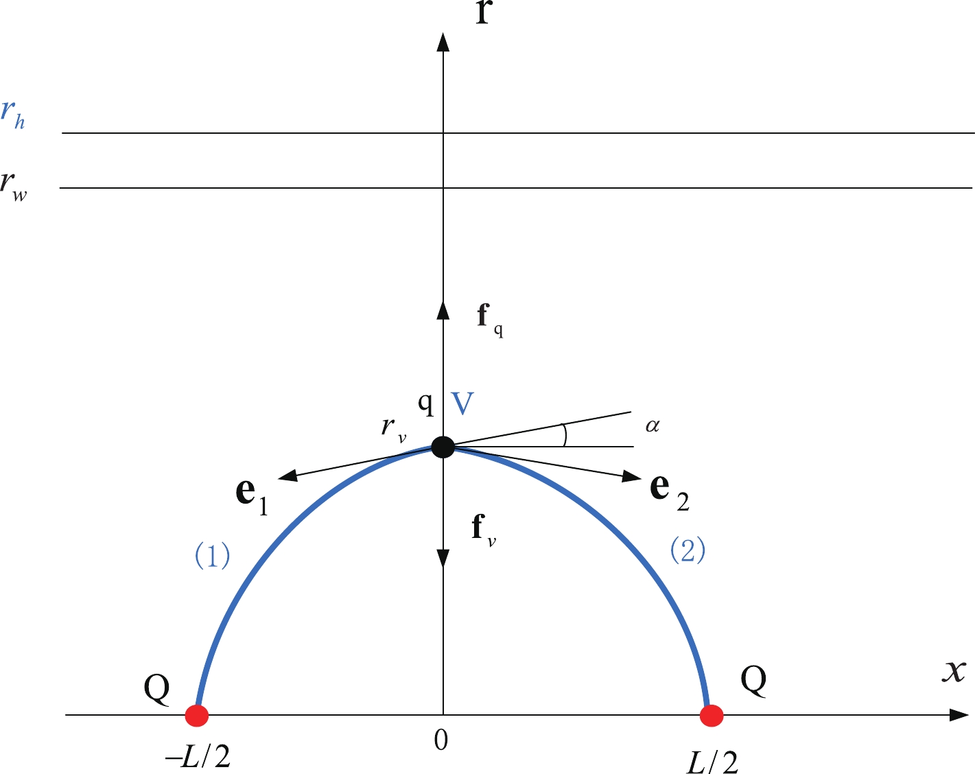
Figure 2. (color online) Static string configuration at an intermediate separation distance of a heavy-quark pair. The heavy quarks Q are placed on the x-axis, while the light quark q and baryon vertex V are at the same point
$r_v$ on the r-axis. The forces exerted on the point are depicted by the black arrows.$r_h$ is the position of the black-hole horizon.$r_w$ is the position of a soft wall in the confined phase.$ S=\sum\limits_{i=1}^{2} S_{{\rm{NG}}}^{(i)}+S_{\rm{vert}}+S_{q}. $

(20) We still choose the same static gauge as before. The boundary conditions then take the form
$ x^{(1)}(0)=-\frac{L}{2}, \quad x^{(2)}(0)=\frac{L}{2} , \quad x^{(i)}\left(r_{v}\right)=0. $

(21) In this configuration, the expressions (11) and (13) still hold. Naturally, we can express the total energy of the string without the contribution from string (3) as follows:
$ \begin{aligned}[b] E_{Q Qq}=&{\boldsymbol{g}} (2\int_{0}^{r_{v}}\left(\frac{1}{r^{2}} {\rm{e}}^{{\boldsymbol{s}} r^{2}} \sqrt{1+f(r)\left(\partial_{r} x\right)^{2}}-\frac{1}{r^2}\right){\rm d} r - \frac{2}{r_v}\\ & + {n} \frac{{\rm{e}}^{\frac{1}{2} s r_v^2}}{r_v} \sqrt{f(r_v)} +3 {k} \frac{{\rm{e}}^{-2 s r_v^2}}{r_v}\sqrt{f(r_v)})+2 c. \end{aligned} $

(22) The force balance equation at the point
$ r = r_v $ is$ {\boldsymbol{e}}_{1}+{\boldsymbol{e}}_{2}+{\boldsymbol{f}}_{v}+{\boldsymbol{f}}_{q}=0. $

(23) Each force is given by
$ {\boldsymbol{f}}_{q}=\left(0,-n {\boldsymbol{g}} \partial_{r_{q}}\left(\frac{{\rm{e}}^{\frac{1}{2} s r_{q}^{2}}}{r_{q}} \sqrt{f\left(r_{q}\right)}\right)\right), $

$ {\boldsymbol{f}}_{v}=\left(0,-3 {\boldsymbol{g}} k \partial_{r_{v}}\left(\frac{{\rm{e}}^{-2 s r_{v}^{2}}}{r_{v}} \sqrt{f\left(r_{v}\right)}\right)\right), $

$ {\boldsymbol{e}}_{1}={\boldsymbol{g}} w\left(r_{v}\right)\left(-\frac{f(r_{v})}{\sqrt{{\rm tan}^2 \alpha + f(r_{v})}},-\frac{1}{\sqrt{f(r_{v}) {\rm cot}^2 \alpha + 1}}\right), $

$ {\boldsymbol{e}}_{2}={\boldsymbol{g}} w\left(r_{v}\right)\left(\frac{f(r_{v})}{\sqrt{{\rm tan}^2 \alpha + f(r_{v})}},-\frac{1}{\sqrt{f(r_{v}) {\rm cot}^2 \alpha + 1}}\right), $

where
$ r_{q} = r_{v} $ . The force balance equation leads to$ \begin{aligned}[b] &2(-{\rm e}^{({5 r_v^2 s})/{2}} n (-1 + r_v^2 s)+3 k (1+4r_v^2 s))\sqrt{f(r_v)}\\-&\frac{4{\rm e}^{3r_v^2 s}}{\sqrt{1+{\rm cot}\alpha^2 f(r_v)}}-\frac{(3k+{\rm e}^{({5r_v^2 s})/{2}})r_v f'(r_v)}{\sqrt{f(r_v)}}=0. \end{aligned} $

(24) -
The total action of the configuration plotted in Fig. 3 is the same as Eq. (20). However, it is convenient to choose another static gauge
$ \xi^{1}=t $ and$ \xi^{2}=x $ here. Then, the boundary conditions are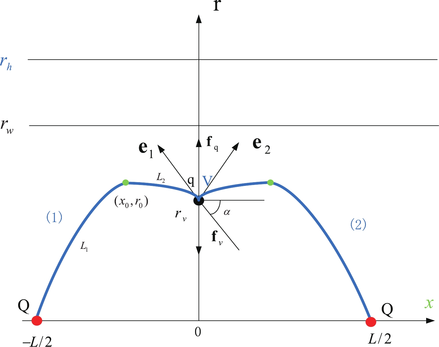
Figure 3. (color online) Static string configuration at a large separation distance of a heavy-quark pair. The heavy quarks Q are placed on the x-axis, while the light quark q and baryon vertex V are at the same point
$r_v$ on the r-axis. The forces exerted on the point are depicted by the black arrows. There is a turning point located at$(x_0, r_0)$ for string (1).$r_w$ is the position of a soft wall in the confined phase.$r_h$ is the position of the black-hole horizon.$ r^{(1)}(-L / 2)=r^{(2)}(L / 2)=0, \quad r^{(i)}(0)=r_{v} . $

(25) The total action becomes
$ \begin{aligned}[b] S=&{\boldsymbol{g}} T\Bigg(\int_{-L / 2}^{0} {\rm d} x w(r) \sqrt{f(r)+\left(\partial_{x} r\right)^{2}}\\&+\int_{0}^{L / 2} {\rm d} x w(r) \sqrt{f(r)+\left(\partial_{x} r\right)^{2}}\\ & +3 {k} \frac{{\rm{e}}^{-2 s r_{v}^{2}}}{r_{v}}\sqrt{f(r_v)}+{n} \frac{{\rm{e}}^{\frac{1}{2} {\rm{s}} r_{v}^{2}}}{r_{v}}\sqrt{f(r_v)}\Bigg). \end{aligned} $

(26) We consider string (1), whose action is given by the first term in (26). The first integral has the form
$ {\cal{I}}=\frac{w(r)f(r)}{\sqrt{f(r)+\left(\partial_{x} r\right)^{2}}}. $

(27) At points
$ r_0 $ and$ r_v $ , we have$ \frac{w(r)f(r)}{\sqrt{f(r)+\left(\partial_{x} r\right)^{2}}}=w(r_0)\sqrt{f(r_0)}, $

(28) $ \frac{w(r_v)f(r_v)}{\sqrt{f(r_v)+ {\rm tan}\alpha^2}}=w(r_0)\sqrt{f(r_0)}. $

(29) The relationship between
$ r_0 $ ,$ r_v $ , and α can be obtained from Eq. (29). Using Eq. (28), the separation distance and energy can be subsequently obtained. As before,$ \partial_x r $ can be solved as$ \partial_x r =\sqrt{\frac{w(r)^2f(r)^2f(r_0) - f(r)w(r_0)^2 f(r_0)^2}{w(r_0)^2 f(r_0)^2}}. $

(30) The separation distance consists of two parts:
$ \begin{aligned}[b] L =& 2(L_1 + L_2) = 2\left(\int_0^{r_0} \frac{1}{r^{\prime}} {\rm d}r + \int_{r_v}^{r_0} \frac{1}{r^{\prime}} {\rm d}r\right)\\ =&2\left(\int_0^{r_0} \sqrt{\frac{w(r_0)^2 f(r_0)^2}{w(r)^2f(r)^2f(r_0) - f(r)w(r_0)^2f(r_0)^2}} {\rm d}r \right.\\ & + \left.\int_{r_v}^{r_0} \sqrt{\frac{w(r_0)^2 f(r_0)^2}{w(r)^2f(r)^2f(r_0) - f(r)w(r_0)^2f(r_0)^2}} {\rm d}r\right). \end{aligned} $

(31) The energy of string (1) can be obtained by summing two parts.
$ \begin{aligned}[b] E_R =& E_{R_1} + E_{R_2}\\ =&{\boldsymbol{g}} \int_0^{r_0} w(r)\sqrt{1 + f(r) x^{\prime 2}} {\rm d}r + {\boldsymbol{g}} \int_{r_v}^{r_0} w(r)\sqrt{1 + f(r) x^{\prime 2}} {\rm d}r \\ =&{\boldsymbol{g}} \int_0^{r_0} w(r) \sqrt{\frac{w(r)^2 f(r)^2 f(r_0)}{w(r)^2f(r)^2f(r_0) - f(r) w(r_0)^2 f(r_0)^2}} {\rm d}r \\ & + {\boldsymbol{g}} \int_{r_v}^{r_0} w(r) \sqrt{\frac{w(r)^2 f(r)^2 f(r_0)}{w(r)^2f(r)^2f(r_0) - f(r) w(r_0)^2 f(r_0)^2}} {\rm d}r . \end{aligned} $

(32) After subtracting the divergent term, the renormalized energy of string (1) is
$ \begin{aligned}[b] E =&{\boldsymbol{g}} \int_{r_v}^{r_0} \Bigg(w(r) \sqrt{\frac{w(r)^2 f(r)^2 f(r_0)}{w(r)^2f(r)^2f(r_0) - f(r) w(r_0)^2 f(r_0)^2}}\Bigg) {\rm d}r \\&+{\boldsymbol{g}} \int_0^{r_0} \Bigg( w(r) \sqrt{\frac{w(r)^2 f(r)^2 f(r_0)}{w(r)^2f(r)^2f(r_0) - f(r) w(r_0)^2 f(r_0)^2}}\\ &- \frac{1}{r^2}\Bigg) {\rm d}r - \frac{1}{r_0}+ 2c. \end{aligned} $

(33) The calculation of string (2) has the same procedure as before and gives the same expressions for L and E. Then, the total energy of the configuration can be written as
$ \begin{aligned}[b] E_{QQq} =& \Bigg{(} 2\int_{r_v}^{r_0} w(r) \sqrt{\frac{w(r)^2 f(r)^2 f(r_0)}{w(r)^2f(r)^2f(r_0) - f(r) w(r_0)^2 f(r_0)^2}} {\rm d}r\\&+ 2\int_0^{r_0} \Bigg(w(r) \sqrt{\frac{w(r)^2 f(r)^2 f(r_0)}{w(r)^2f(r)^2f(r_0) - f(r) w(r_0)^2 f(r_0)^2}} \\& - \frac{1}{r^2}\Bigg) {\rm d}r - \frac{1}{r_0}+ 3 {k} \frac{{\rm{e}}^{-2 \;{\rm{s}} r_{v}^{2}}}{r_{v}}+{n} \frac{{\rm{e}}^{\frac{1}{2} {\boldsymbol{s}} r_{v}^{2}}}{r_{v}}\Bigg){\boldsymbol{g}} + 2c. \end{aligned} $

(34) The force balance equation is the same as Eq. (23). Each force is similarly given in the previous section. With Eq. (29) and (24), we can numerically solve L and
$ E_{QQq} $ .Except in the symmetric case, the light quark can be in a position far from the r-axis. The non-symmetric configuration has been discussed in Ref. [33], which, as noted in Ref. [33], is not energetically favorable. In this paper, we mainly focus on the symmetric configuration.
-
The system will change from the confined to deconfined phase with increasing temperature. The procedure for determining the melting temperature of QQq is similar to that of
$ {Q\bar{Q}} $ . We can judge the meting temperature from the behavior of the potential energy. In the confined phase, if we do not consider string breaking, the potential will rise linearly forever. When changing from a low to high temperature, the behavior of the potential will have an endpoint, as shown in the figures of Sec. III.B.3. Besides the potential, we can also judge the melting temperature from the behavior of the separation distance. Further discussions can be found in [6, 8, 16, 19].In this section, we investigate the effect of different temperatures on the QQq potential. The configurations of QQq change with temperature. With an increase in temperature, QQq melts. Because we want to approach the lattice at vanishing temperature, all the parameters are fixed as follows:
$ s = 0.42\;{\rm{GeV}}^2 $ ,$ {\boldsymbol{g}} = 0.176 $ ,$ n = 3.057 $ ,$ k = -\dfrac{1}{4}{\rm e}^{{1}/{4}} $ , and$ c = 0.623\;{\rm GeV} $ [33]. -
First, we investigate the configurations of QQq at the low temperature
$ T=0.1\;{\rm GeV} $ . At this temperature, the system is in the confined phase with a soft wall below the black-hole horizon, and the string and light quark cannot exceed this wall [6, 8, 16, 19]. -
From (17), we can determine the position of the light quark at fixed temperature. The force balance equation of the light quark
$ F_l(r_q) $ as a function of$ r_q $ is presented in Fig. 4(a), where two solutions are observed. However, one solution beyond the soft wall is unphysical. At temperature$ T=0.1\;{\rm{GeV}} $ ,$ r_q = 1.15\;{\rm{ GeV}}^{-1} $ is a solution of the force balance equation. Then, α can be numerically solved from Eq. (19). The force balance equation for the vertex can give the relationship between the angle α and$ r_v $ , as shown in Fig. 4(b). In the range$ 0 \leq r_v \leq r_q $ , we find that α is not a monotone function of$ r_v $ ; it first decreases and then increases with an increase in$ r_v $ . A schematic diagram is shown in Fig. 5.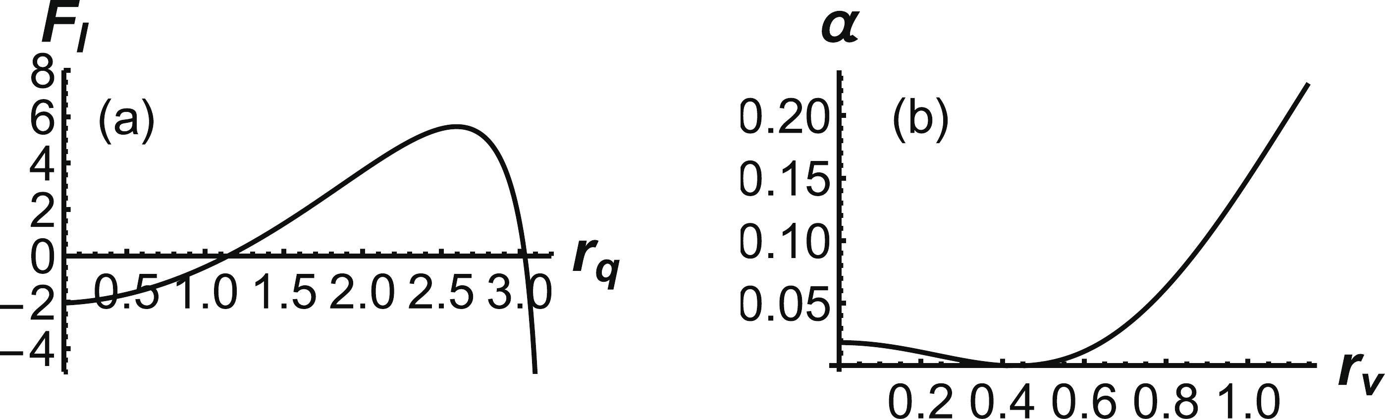
Figure 4. (a) Force balance equation of the light quark as a function of
$ r_q $ . (b) α as a function of$ r_v $ . The unit for$ r_q $ and$ r_v $ is$ \rm{GeV^{-1}} $ .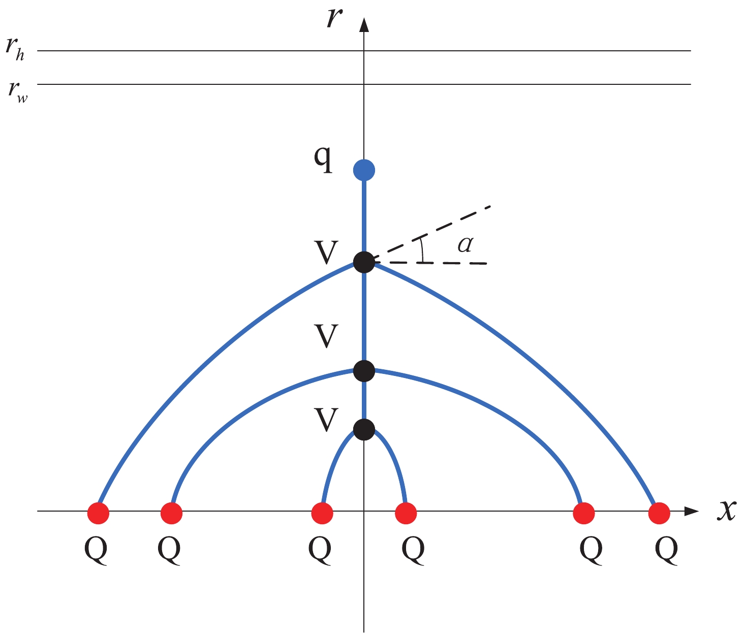
Figure 5. (color online) Schematic diagram of the string configuration with increasing
$ r_v $ for small L. α is always positive.Furthermore, the separation distance of a heavy-quark pair, which can be calculated using Eq. (11), is shown inFig. 6(a). L is a monotonously increasing function of
$ r_v $ . At$ r_v = r_q $ , there is a cutoff. Beyond$ r_q $ , the configuration will turn into the second case. The corresponding energy can be calculated using Eq. (15), which is shown in Fig. 6 (b). It is found that the energy is a Coulomb potential at small separation distances and a linear potential at large distances.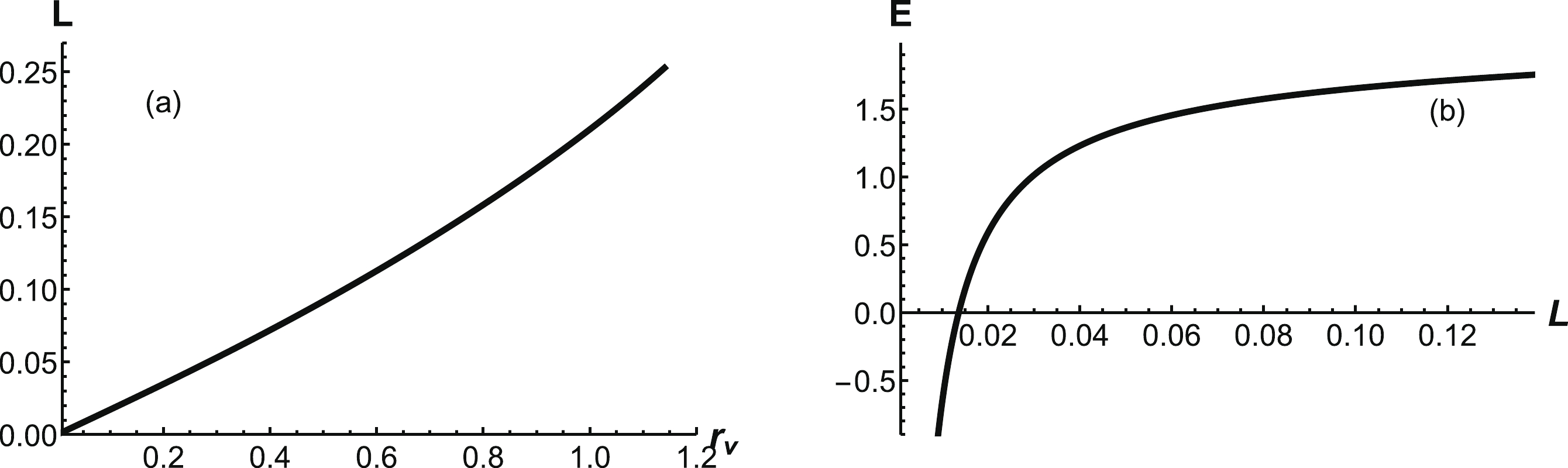
Figure 6. (a) Separation distance L as a function of
$ r_v $ . (b) Energy E as a function of separation distance L. The unit of E is$ {\rm{GeV}} $ , the unit of L is$ {\rm{fm}} $ , and that of$ r_v $ is$ \rm{GeV^{-1}} $ . -
In the second configuration,
$ r_v $ ranges from$ r_q $ to a certain position where α vanishes, as shown in Fig. 7. A schematic diagram for this case is shown in Fig. 8. At the beginning,$ \alpha \approx 0.22 $ . When we increase$ r_v $ , α slowly tends to zero.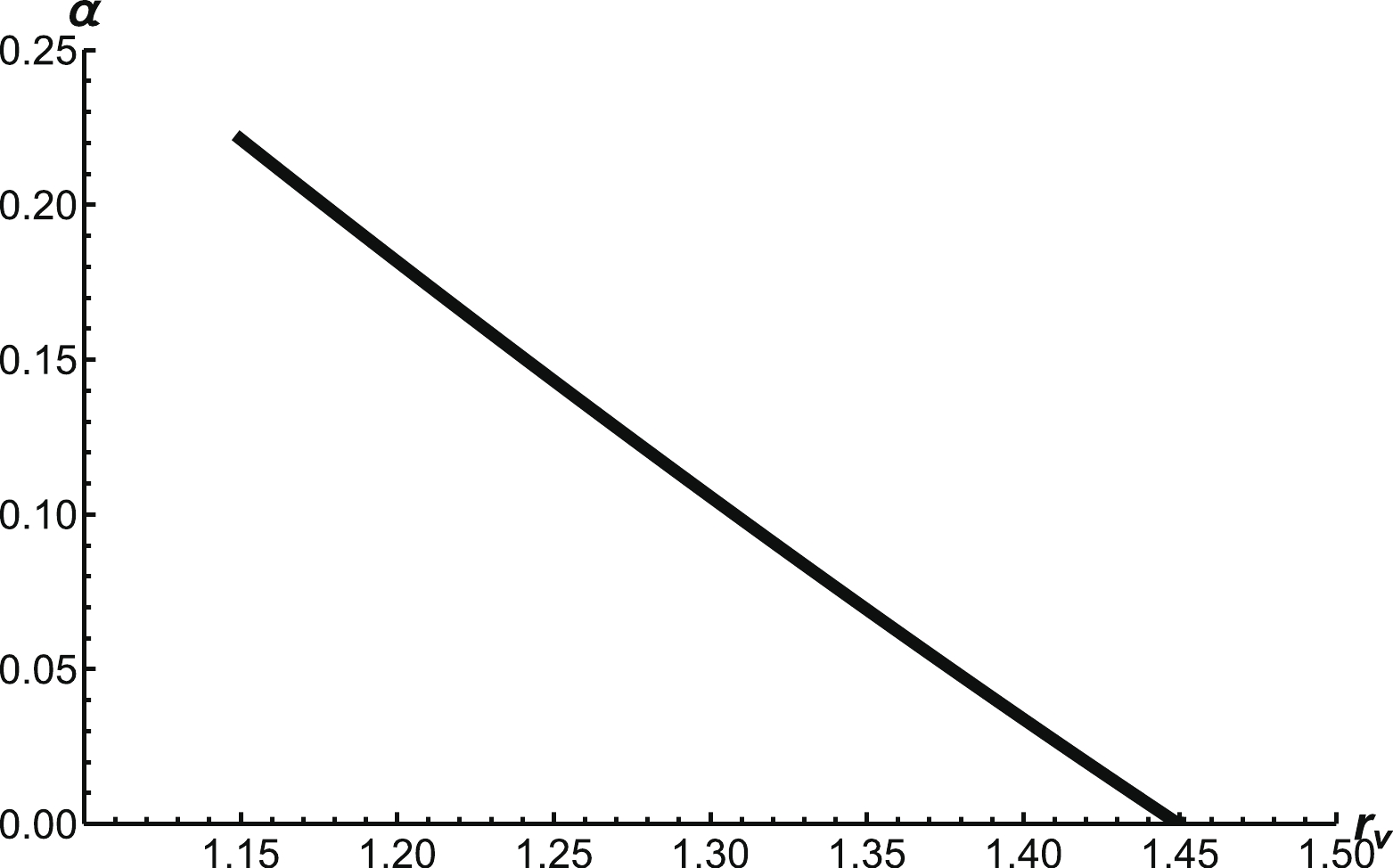
Figure 7. α as a function of
$r_v$ . The unit of$r_v$ is$\rm{GeV^{-1}}$ .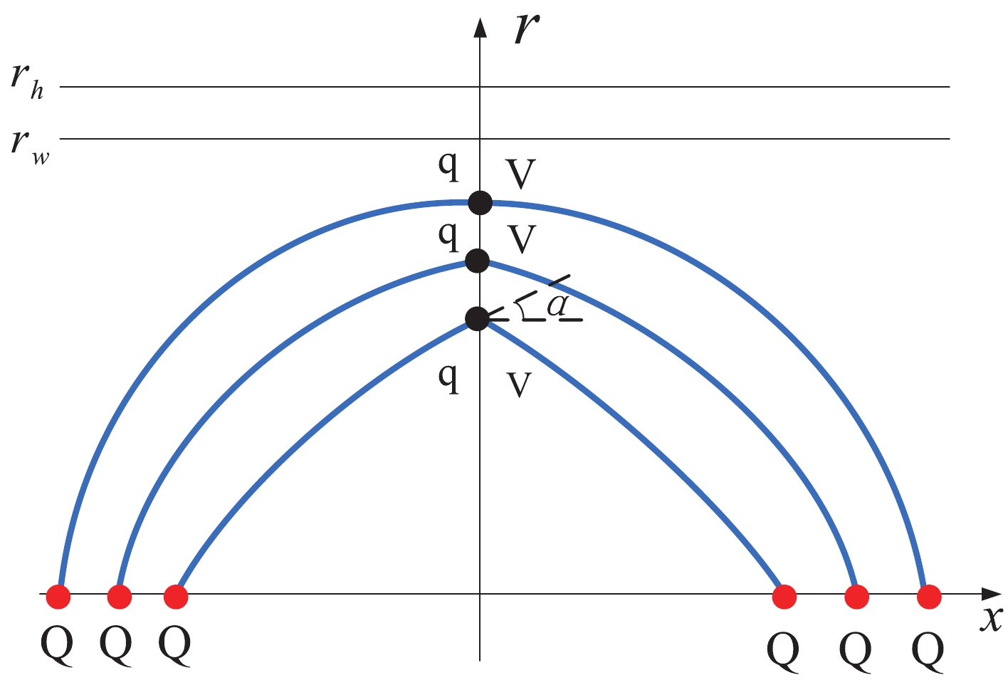
Figure 8. (color online) Schematic diagram of the string configuration with increasing
$r_v$ for intermidiate$L$ . α is always positive.The separation distance of a heavy-quark pair can also be calculated from Eq. (11). In Fig. 9(a), we can see that L increases with an increase in
$ r_v $ . There is an endpoint$ r_v = 1.45 \;\rm{GeV^{-1}} $ , where α tends to zero. Similarly, by solving the force balance equation of (24), we obtain numerical results for α. It is found that α is a monotone function of$ r_v $ and decreases with an increase in$ r_v $ . From Fig. 9(a), it is clear that the separation distance will increase with increasing$ r_v $ . It should be noted that$ r_v $ has a maximum value, beyond which the configuration will turn to the third case. The maximum separation distance and energy emerge at$ r_v =1.45\; \rm{GeV^{-1}} $ . The corresponding energy can also be evaluated, which is shown in Fig. 9(b). In this configuration, the energy is a linear function of L. Next, we turn to the third case and discuss it further.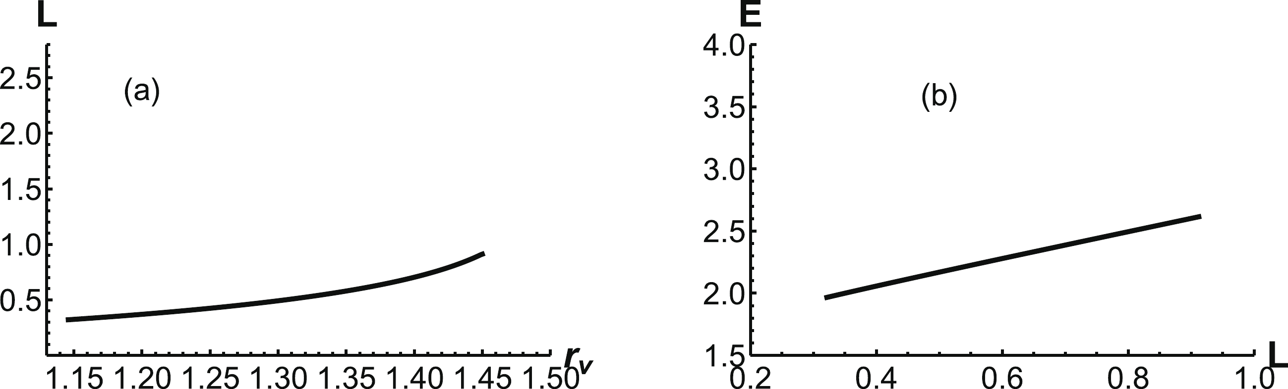
Figure 9. (a) Separation distance L as a function of
$ r_v $ . (b) The energy E as a function of L. The unit of E is$ {\rm{GeV}} $ , the unit of L is$ {\rm{fm}} $ , and that of$ r_v $ is$ \rm{GeV^{-1}} $ . -
Using Eq. (24), we first numerically obtain the relationship between α and
$ r_v $ , as shown in Fig. 10(a). Unlike the previous case, the difference here is a negative α. Calculating the first integral from Eq. (29), we find that$ r_0 $ is a function of$ r_v $ in Fig. 10(b). As shown, the maximum$ r_v $ is$ r_v \approx 1.48\;{\rm{GeV}}^{-1} $ , which corresponds to the position of the soft wall$ r_w \approx r_0 \approx 1.53 {\rm{GeV}}^{-1} $ . We can also see that the separation distance tends to infinity when$ r_0 $ approaches$ 1.53 \;{\rm{GeV}}^{-1} $ in Fig. 11(a).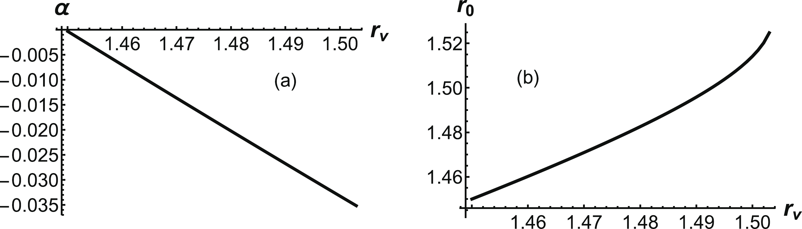
Figure 10. (a) α as a function of
$ r_v $ .$ r_0 $ as a function of$ r_v $ .$ r_0 $ and$ r_v $ have the unit of$ {\rm GeV}^{-1} $ .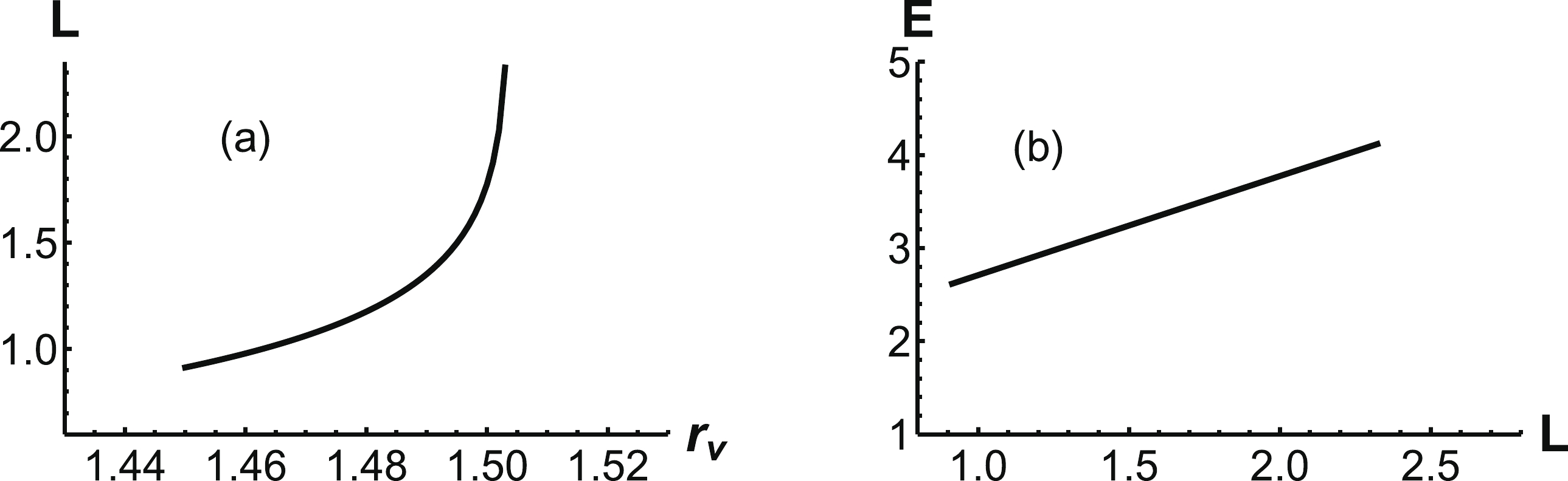
Figure 11. (a) Separation distance L as a function of
$ r_v $ . (b) The energy E as a function of L. The unit of E is$ {\rm{GeV}} $ , the unit of L is$ {\rm{fm}} $ , and that of$ r_v $ is$ \rm{GeV^{-1}} $ .Finally, the corresponding potential energy is shown in Fig. 11(b). Because the absolute value of α decreases with increasing
$ r_v $ , we present a schematic diagram of the third configuration in Fig. 12. At$ r_0 \approx r_w $ , α tends to zero, and the separation distance becomes extremely large.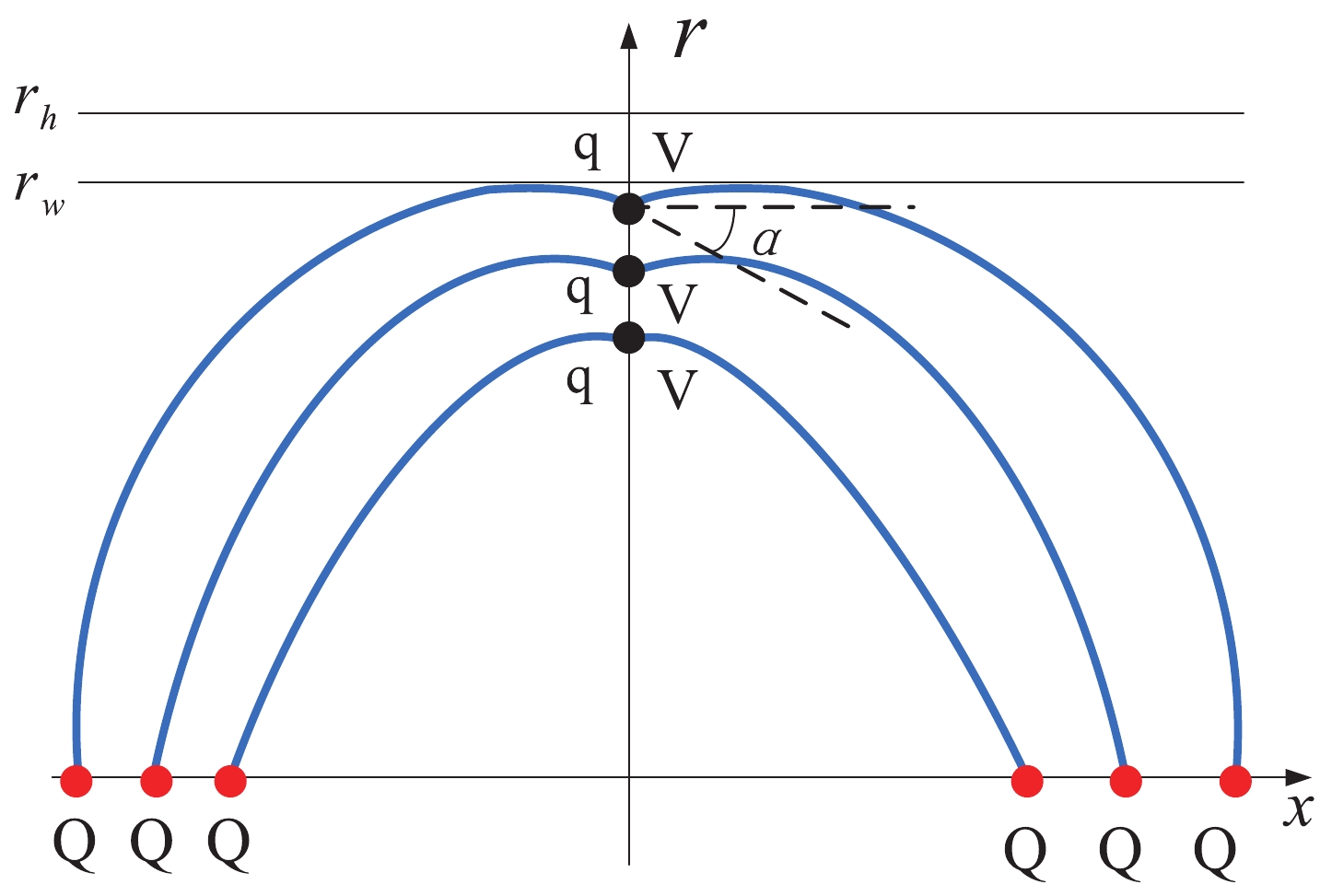
Figure 12. (color online) Schematic diagram of the string configuration with increasing
$r_v$ for large L. α is always negative. -
If we combine all the configurations, we can present the energy as a function of L at all distances, as shown in Fig. 13. Clearly, the energy is smoothly increasing with separation distance for all configurations.

Figure 13. (color online) Energy E as a function of L at all separation distances. The black line represents small distances, the blue line represents intermediate distances, and the red line represents large distances. The unit of E is GeV, and the unit of L is fm.
-
At temperature
$ T=0.148\;{\rm{GeV}} $ , the system is in the deconfined phase. In this phase, the soft wall disappears, and QQq will melt at a sufficient distance. -
First, we can determine the position of the light quark from (17). At
$ T=0.148\;{\rm{GeV}} $ , we find$ r_q = 1.38 {\rm{ GeV}}^{-1} $ or$ r_q = 1.54 \;{\rm{GeV}}^{-1} $ . In this study, we focus on the ground state and only consider$ r_q = 1.38 \;{\rm{GeV}}^{-1} $ at$ T=0.148 {\rm{GeV}} $ . The angle α can be calculated from Eq. (19). The energy and separation distance are calculated using the same procedure as before, and the results are shown in Fig. 14. L is still an increasing function of$ r_v $ , and E is a Cornell-like potential.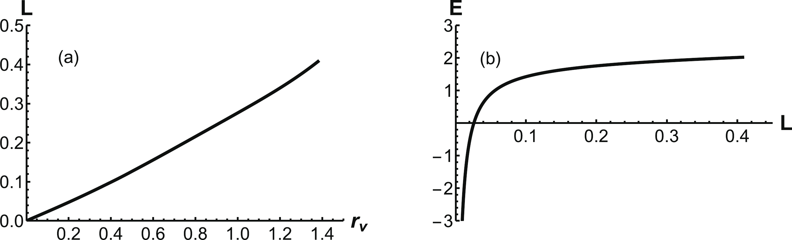
Figure 14. (a) Separation distance L as a function of
$ r_v $ . (b) The energy E as a function of L. The unit of E is$ {\rm{GeV}} $ , the unit of L is$ {\rm{fm}} $ , and that of$ r_v $ is$ \rm{GeV^{-1}} $ . -
In this configuration, we calculate the energy and separation distance in Fig. 15. With an increase in
$ r_v $ , the separation distance increases. There is a maximum value$ L_{\rm max} = 0.445\; {\rm{fm}} $ beyond which the configuration cannot exist and quarks become free. Thus, we find that the third configuration cannot exist at$ T= 0.145 \;{\rm GeV} $ .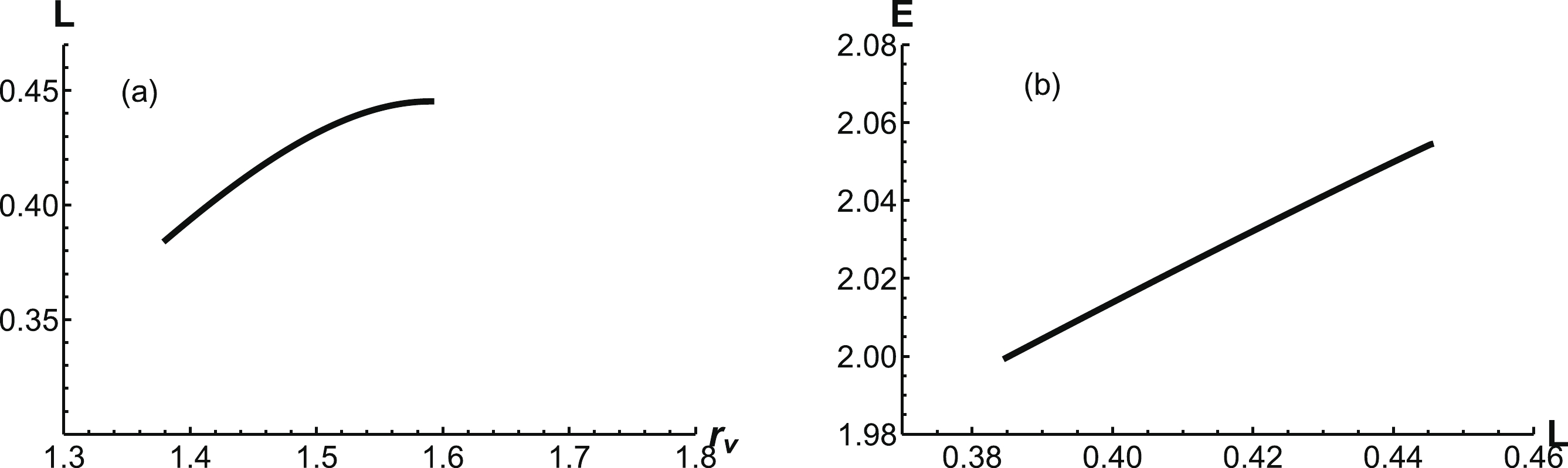
Figure 15. (a) Separation distance L as a function of
$ r_v $ . (b) The energy E as a function of L. The unit of E is$ {\rm{GeV}} $ , the unit of L is$ {\rm{fm}} $ , and that of$ r_v $ is$ \rm{GeV^{-1}} $ . -
Only the first and second configurations can exist at
$ T = 0.148\;{\rm{GeV}} $ . We present the energy as a function of separation distance from 0 to$ L_{\rm max} $ in Fig. 16. The potential is smoothly increasing from small distances to intermediate distances. The potential ends at$ L_{\rm max} = 0.445\;{\rm{fm}} $ , marked by the red dot in the figure. At large distances, QQq melts and becomes free quarks.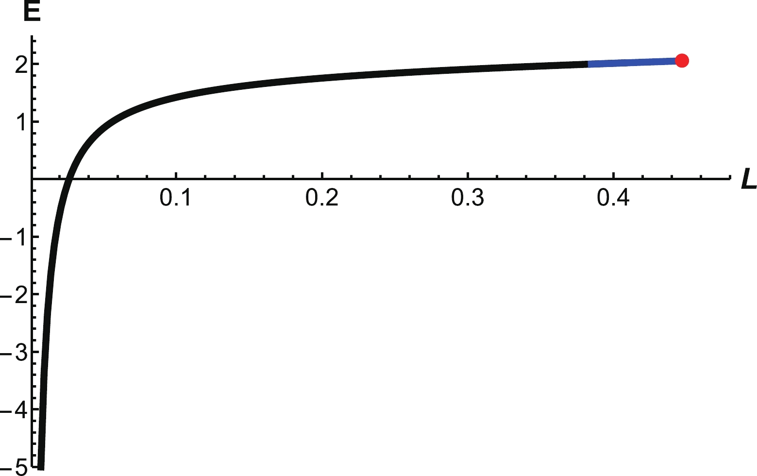
Figure 16. (color online) Energy E as a function of L at all distances. The black line represents
$E_{QQq}$ at small distances, the blue line represents$E_{QQq}$ at intermediate distances, and the red line represents$E_{QQq}$ at large distances. The unit of E is GeV, and the unit of L is fm. -
First, we check the force balance equation of the light quark for the first configuration and find there is no solution for any
$ r_q $ at$ T=0.15\;{\rm GeV} $ , as shown in Fig. 17. Thus, the first configuration cannot exist at this temperature. From Eq. (24), we can find the relationship between α and$ r_v $ . There is also a maximum value$ r_{\rm max} $ at$ T=0.15\;{\rm GeV} $ , beyond which QQq meltsas shown in Fig. 18. The separation distance and energy of the string are shown in Fig. 19.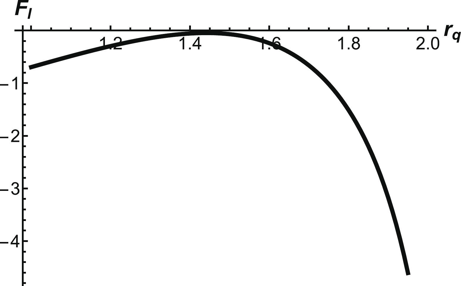
Figure 17. Force balance equation of the light quark as a function of
$r_q$ . The unit of$r_q$ is${\rm{GeV}}^{-1}$ .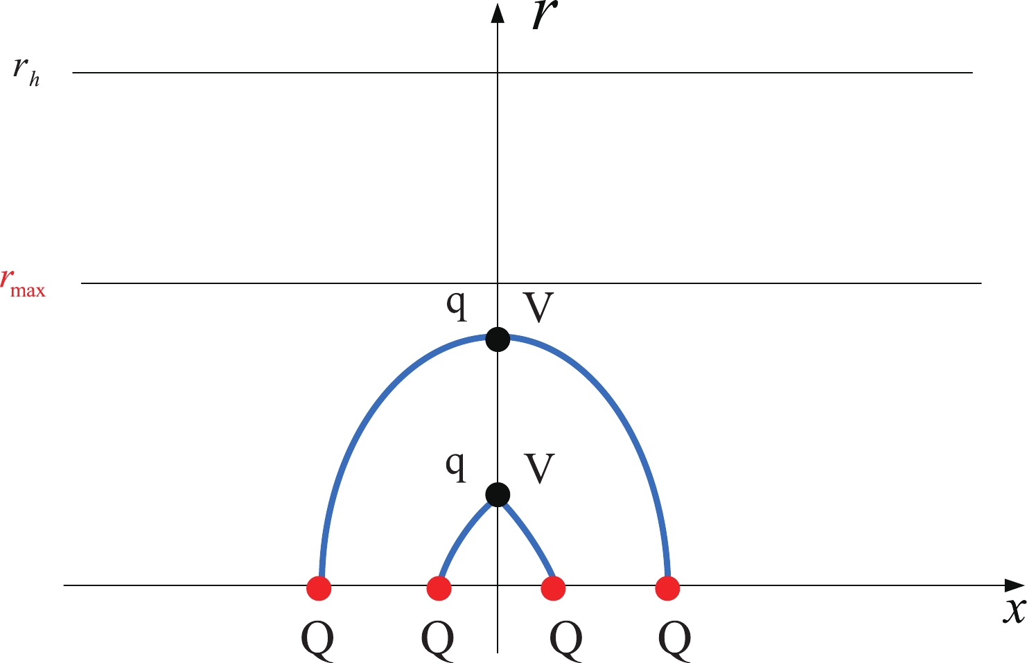
Figure 18. (color online) Schematic diagram of the string configuration with increasing
$r_v$ .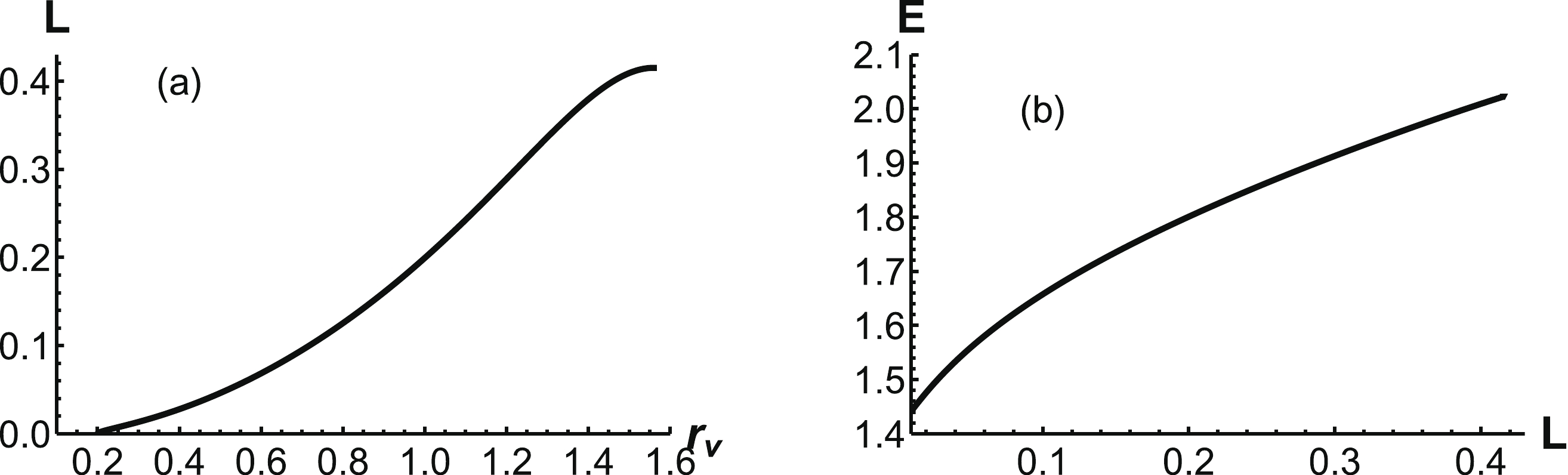
Figure 19. (a) Separation distance L as a function of
$ r_v $ . (b) The energy E as a function of L. The unit of E is$ {\rm{GeV}} $ , the unit of L is$ {\rm{fm}} $ , and that of$ r_v $ is$ \rm{GeV^{-1}} $ . -
In the confined phase, the quarks are confined in the hadrons. Can QQq exist at extremely large distances? The answer is no. The light quarks and anti-quark will be excited from vacuum at large distances. We call this string breaking and consider the following decay mode:
$ Q Q q \rightarrow Q q q+Q \bar{q}. $

(35) Qqq consists of three fundamental strings: a vertex and two light quarks. Thus, the total action of Qqq is
$ S=\sum_{i=1}^{3} S_{{\rm{NG}}}^{(i)}+S_{\rm{vert}}+2S_{\rm{q}} $ .$ Q\bar{q} $ consists of a fundamental string and a light quark. Thus, the total action of Qqq is$ S= S_{{\rm{NG}}}+S_{q} $ . The total actions of$ Qqq $ and$ Q\bar{q} $ are$ \begin{aligned}[b] S_{ {Qqq} }=& {\boldsymbol{g}} \Bigg(2 \int_{r_v}^{r_q} \frac{{\rm e}^{s r^2}}{r^2} {\rm d}r + \int_{0}^{r_v} \frac{{\rm e}^{s r^2}}{r^2}+ 3k \frac{{\rm e}^{-2 s r_v^2} \sqrt{f(r_v)}}{r_v}\\&+2 n \frac{{\rm e}^{\frac{1}{2}s r_q^2}}{r_q} \sqrt{f(r_q)}\Bigg), \\ {S_ {Q\bar{q}} }=& {\boldsymbol{g}} \int_{0}^{r_q}\frac{{{\rm e}^{s r^2}}}{r^2} + n {\boldsymbol{g}} \frac{{\rm e}^{\frac{1}{2}s r_q^2}}{r_q} \sqrt{f(r_q)} . \end{aligned} $

(36) Varying the action with respect to
$ r_q $ gives Eq. (17), and varying the action with respect to$ r_v $ gives$ \begin{aligned}[b] &1 + 3k {\rm e}^{-3 s r_v^3} \sqrt{f(r_v)} + 12 k s {\rm e}^{-3 s r_v^3} r_v^2\sqrt{f(r_v)}\\ -& \frac{3 k {\rm e}^{-3 s r_v^2} r_v f'(r_v)}{2\sqrt{f(r_v)}} = 0. \end{aligned} $

(37) We can obtain
$ r_v=0.410 \;{\rm{GeV}}^{-1} $ or$ r_v=0.453\;{\rm{ GeV}}^{-1} $ . Because the difference in energy is extremely small for the two states, we take$ r_v=0.410\;{\rm{GeV}}^{-1} $ for simplicity. The configuration for$ Q q q+Q \bar{q} $ is shown in Fig. 20. The renormalized total energy is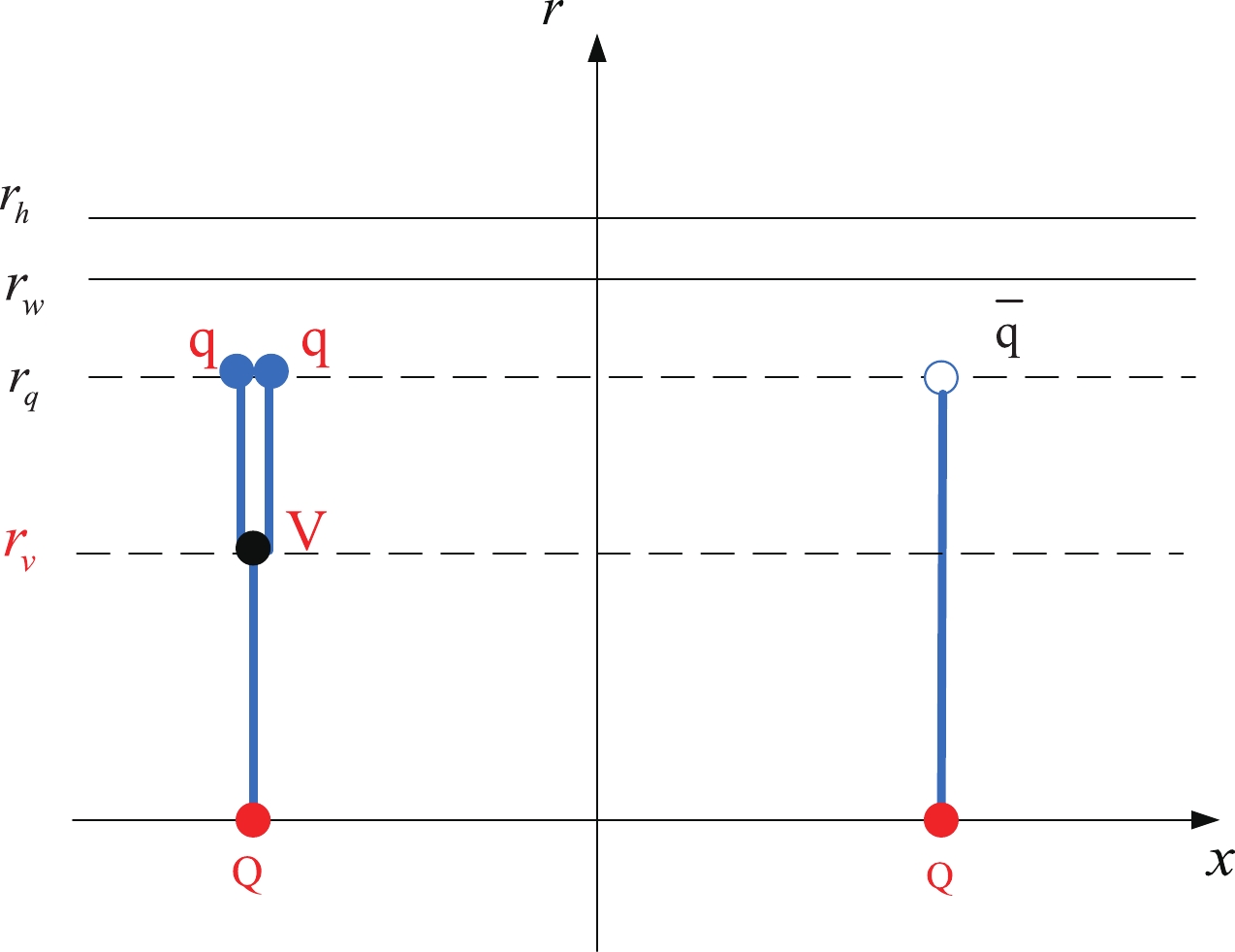
Figure 20. (color online) Schematic diagram of
$Q q q+Q \bar{q}$ .$ \begin{aligned}[b] E_{ {Qqq}}+E_{ {Q\bar{q}}} =& {\boldsymbol{g}} \Bigg(2 \int_{r_v}^{r_q} \frac{{\rm e}^{s r^2}}{r^2} {\rm d}r + \int_{0}^{r_q}\left(\frac{{{\rm e}^{s r^2}}}{r^2} - \frac{1}{r^2}\right) - \frac{1}{r_q} \\ &+\int_{0}^{r_v} \left(\frac{{\rm e}^{s r^2}}{r^2}-\frac{1}{r^2}\right)- \frac{1}{r_v}+ 3k \frac{{\rm e}^{-2 s r_v^2} \sqrt{f(r_v)}}{r_v}\\& + 3 n \frac{{\rm e}^{\frac{1}{2}s r_q^2}}{r_q} \sqrt{f(r_q)}\Bigg) + 2c. \end{aligned} $

(38) For fixed
$ r_q=1.146 \;{\rm{GeV}}^{-1} $ and$ r_v=0.410\;{\rm{ GeV}}^{-1} $ , we have$ E_{ {Qqq}}+E_{ {Q\bar{q}}} = 3.006\;{\rm{ GeV}} $ . Figure 21 is a schematic diagram of string breaking. To determine the string breaking distance, we plot the energy$ E_{QQq} $ and$ E_{Q\bar{q}}+ E_{Qqq} $ as a function of$ r_v $ at$ T = 0.1\;{\rm{GeV}} $ in Fig. 22. The cross point shown in the figure enables us to determine$ L_{QQq} $ at fixed temperature. We find the distance of string breaking to be$ L_{QQq} = 1.27\; {\rm{fm}} $ .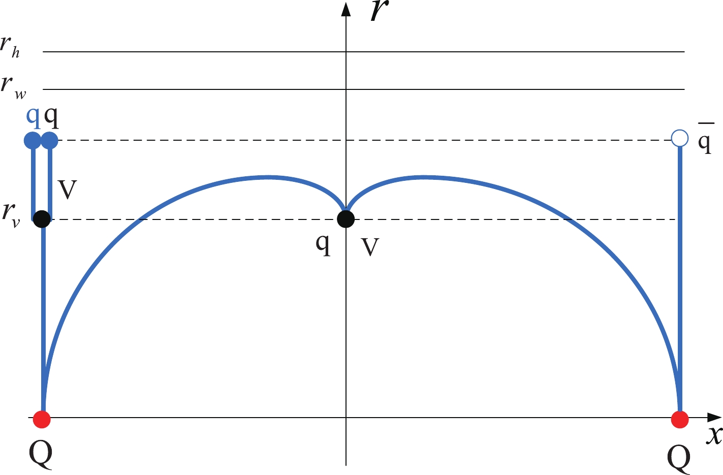
Figure 21. (color online) Schematic diagram of string breaking from the third configuration of QQq to
$Q q q+Q \bar{q}$ .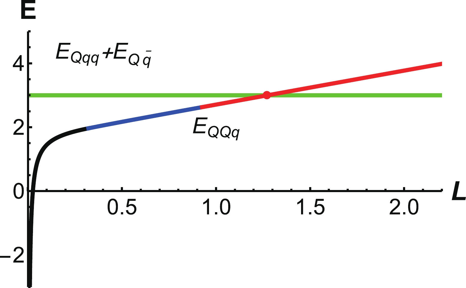
Figure 22. (color online) Green line is the energy
$E_{Qqq}+E_{Q\bar{q}}$ . The black line represents$E_{QQq}$ at small distances, the blue line represents$E_{QQq}$ at intermediate distances, and the red line represents$E_{QQq}$ at large distances. The unit of E is GeV, and the unit of$r_v$ is$\rm GeV^{-1}$ . -
The energy of
$ {Q\bar{Q}} $ has been extensively studied in many holographic models. In this section, we focus on comparing the energy of${Q\bar{Q}} $ with QQq in the confined and deconfined phases. First, we only show the results of the separation distance and energy of$ {Q\bar{Q}} $ $ L_{Q\bar{Q}} = 2 \int_{0}^{r_0} \left(\frac{g_2(r)}{g_1(r)}\left(\frac{g_2(r)}{g_2(r_0)}-1\right)\right)^{-{1}/{2}}, $

(39) $ E_{ {Q\bar{Q}}} =2 {\boldsymbol{g}} \left(\int_{0}^{z_0} \sqrt{\frac{g_2(r) g_1(r)}{g_2(r)-g_2(r_0)}}-\frac{1}{r^2}\right) - \frac{2 {\boldsymbol{g}}}{r_0} + 2c, $

(40) where
$ g_1(r) = \dfrac{{\rm e}^{2 s r^2}}{r^4},\; g_2(r) = \dfrac{{\rm e}^{2 s r^2}}{r^4} f(r) $ , and$ z_0 $ is the turning point of the U-shape string. A detailed calculation can be found in our previous paper [19, 24, 25]. We consider the decay mode$ {Q \bar{Q}\rightarrow Q\bar{q} + \bar{Q}q}. $ It is clear that$ E_{ {Q\bar{q}}} = {\boldsymbol{g}} \left(\int_{0}^{r_q} \frac{1}{r^2}({\rm e}^{s r^2} - 1)\right) -\frac{{\boldsymbol{g}}}{r_q} + {\boldsymbol{g}} n \frac{{\rm e}^{\frac{s}{2}r_q^2}}{rq}\sqrt{f(r_q)} + c. $

(41) Thus, we can calculate
$ E_{ {Q\bar{q}}}+E_{ {\bar{Q}q}} = 2.39 \;{\rm{GeV}} $ at$ T = 0.1\;{\rm{GeV}} $ . In the confined phase, such as when$ T = 0.1\;{\rm{GeV}} $ , we present the energy of$ E_{ {Q\bar{q}}}+E_{ {\bar{Q}q}} $ and$ E_{ {Q\bar{Q}}} $ in Fig. 23. Through a comparison with Fig. 22, we find the distance of string breaking$ L=1.25\; {\rm{fm}} $ is close to that of QQq.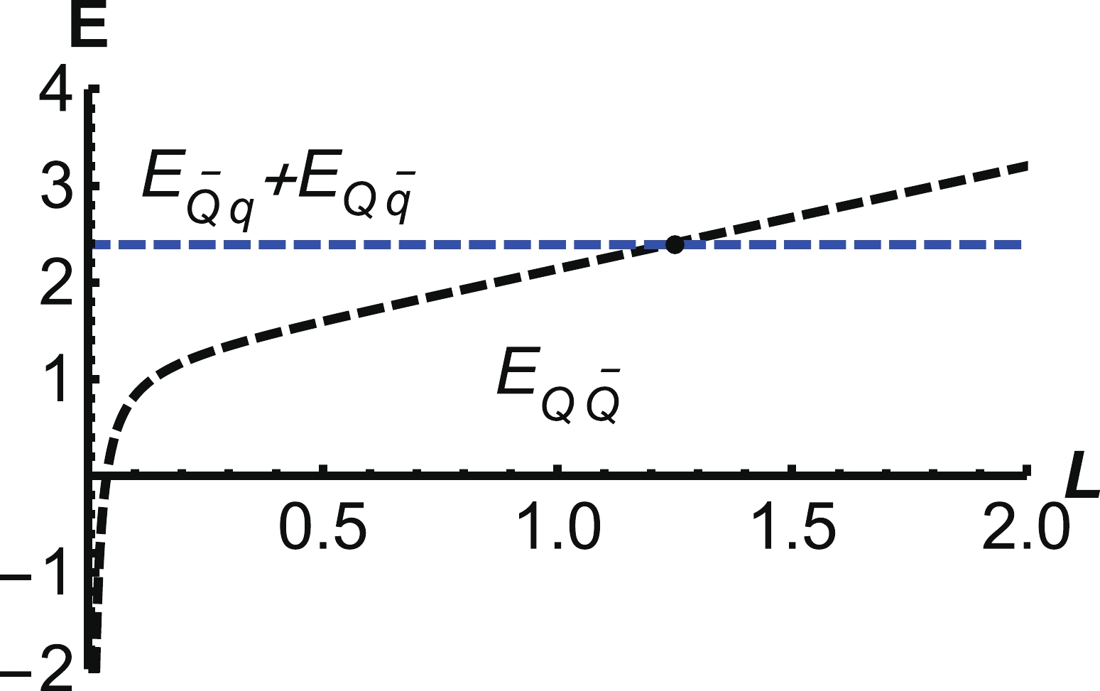
Figure 23. (color online) Blue dashed line is the energy of
$E_{ {Q\bar{q}}}+E_{ {\bar{Q}q}}$ , and the black dashed line is the energy of$E_{ {Q\bar{Q}}}$ . The temperature is$T = 0.1\; \rm{GeV}$ . The unit of E is GeV, and the unit of L is fm.In the deconfinement phase, we compare the energies of
$ E_{ {Q\bar{Q}}} $ and$ E_{ {QQq}} $ at$ T = 0.148\;{\rm{GeV}} $ . Fig. 24 shows that the screening distance of$ E_{ {QQq}} $ ($ L = 0.45\;\rm{fm} $ ) is significantly smaller than that of$ E_{ {Q\bar{Q}}} $ ($ L = 0.94\;\rm{fm} $ ) at the same temperature$ T = 1.48 \;{\rm{GeV}} $ . This indicates that$ {Q\bar{Q}} $ is more stable than QQq in the deconfined phase.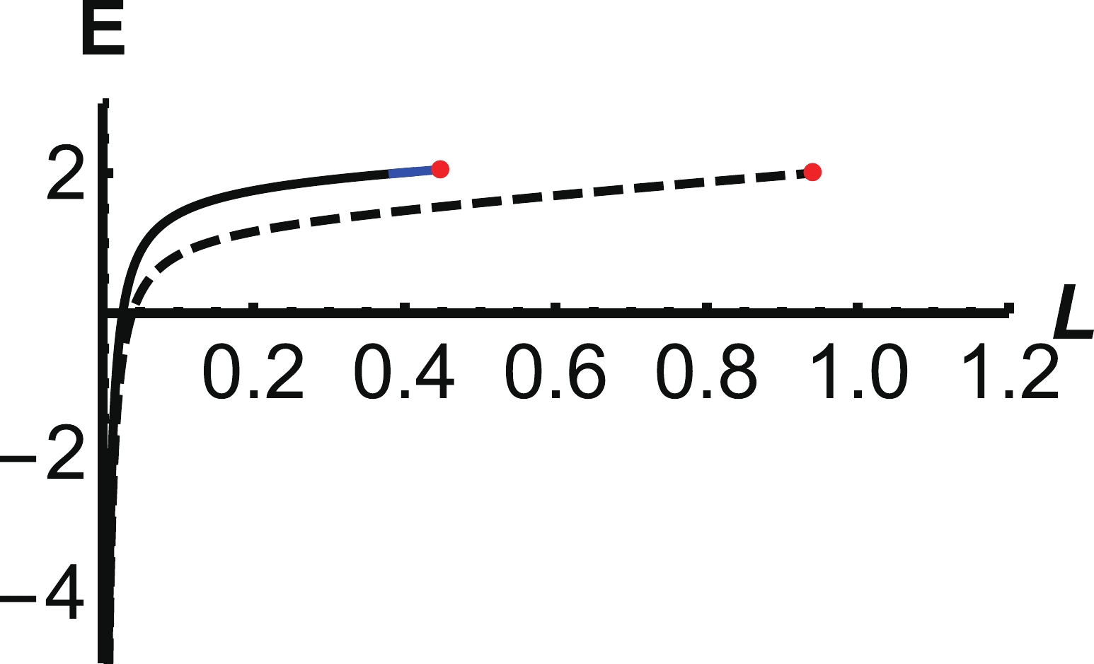
Figure 24. (color online) Solid line is the energy of
$E_{ {QQq}}$ , and the dashed line is the energy of$E_{ {Q\bar{Q}}}$ . The temperature is$T = 0.148\; \rm{GeV}$ . The unit of E is GeV, and the unit of L is fm. -
In this study, we focused on QQq melting and string breaking at finite temperature through a five-dimensional effective string model. For the confined phase, string and light quarks cannot exceed the soft wall. Quarks are permanently confined in the hadrons. However, string breaking of QQq occurs at sufficiently large distances. We considered the decay mode
$ {Q Q q} \rightarrow {Q q q+Q \bar{q}} $ and found the distance of string breaking to be$ L = 1.27\; {\rm{fm}} $ . Other decay modes may be considered in the future studies. At a high temperature, the system is in the deconfined phase, which implies that the soft wall disappears and QQq melts at a certain distance. For example, QQq melts at$ L = 0.45\;\rm{fm} $ for$ T = 0.148\;{\rm{GeV}} $ . In contrast, we found that$ {Q\bar{Q}} $ melts at$ L = 0.94\;\rm{fm} $ for$ T = 0.148\;{\rm{GeV}} $ , which indicates that$ {Q\bar{Q}} $ is more stable than QQq at high temperatures. Finally, we hope that studying the effective string model will provide more observable quantities for future experiments.
Studying the potential of QQq at finite temperature in a holographic model
- Received Date: 2021-12-28
- Available Online: 2022-07-15
Abstract: Using gauge/gravity duality, we investigate the string breaking and dissolution of two heavy quarks coupled to a light quark at finite temperature. It is found that three configurations of QQq exist with the increase in separation distance for heavy quarks in the confined phase. Furthermore, string breaking occurs at the distance


 DownLoad: