


 Abstract
 HTML
HTML Reference
 Related
 PDF
PDF


-
Color glass condensate (CGC) [1–5] is an effective theory for describing physics in the proton saturation regime. Inside a proton, gluons cannot grow infinitely without breaking the unitary limit. Consequently, in the small x regime, the recombination and multiple scattering of gluons reach a balance, and then, the number of gluons does not increase. This is called gluon saturation, which can be described by the CGC effective field theory. For studying the proton structure in the saturation regime at the high energy limit, deep inelastic scattering (DIS), deeply virtual compton scattering (DVCS), and exclusive diffractive vector meson production are excellent probes [6–8].
For analyzing DIS and vector meson production, the color dipole model and CGC effective theory are powerful tools [9–16]. In the dipole model, a virtual photon splits into a quark anti-quark pair (dipole), which interacts with protons by exchanging gluons. Then, the dipole recombines into a meson or photon. The Golec-Biernat and Wusthoff (GBW) model [17] and the CGC model [18] describe the dipole scattering process well. Moreover, two impact-parameter dependent models, the b-CGC model, [19, 20] which is a modification of the CGC model and the IP-Sat [21, 22] model are successful at describing the applications of DIS and the exclusive vector meson production process [18, 23–26]. The saturation effect in the b-CGC model and the IP-Sat model is related to the Balitsky-Kuraev-Fadin-Lipatov (BFKL) equation [27–30] and the Dokshitzer-Gribov-Lipatov-Altarelli-Parisi (DGLAP) equation, [31–33] respectively [34]. These models are also applied to the Large Hadron Collider (LHC) experiment [35–38].
Besides, the evolution of the dipole-target scattering amplitude can be dominated by the Balitsky-Kovchegov (BK) equation [39–42] with a nonlinear term for gluon saturation, which is regarded as the mean field approximation of the Jalilian-Marian-Iancu-McLerran-Weigert-Leonidov-Kovner (JIMWLK) equation [43–46]. There is a considerable amount of research on the BK equation. The influence of the impact parameter b was numerically analyzed for the BK equation in [47]. The solution of the b-dependent BK equation with a collinearly improved kernel has been studied [48]. A discussion of the behavior of the numerical solution of the running coupling BK equation with the Runge-Kutta method was presented in [49]. Reference [50] showed a numerical solution to the BK equation in coordinate space for the next-to-leading order.
In momentum space, it has been shown [40, 41] that the nonlinear evolution equation with the Balitskii-Fadin-Kuraev-Lipatov (BFKL) kernel can be obtained form the BK equation by proper approximation. Then, by variable substitution, this nonlinear evolution equation [51–53] is simplified to the Fisher-Kolmogorov-Petrovsky-Piscounov (FKPP) equation, [54] which is a kind of reaction-diffusion nonlinear equation. The analytical solution of the BK equation is obtained by solving the more concise FKPP equation. The analytical solution [55–59] of the BK equation has been studied by different methods. We also obtain the analytical solution of the BK equation [60] in momentum space. In this work, the analytical solution that we have obtained is used to explain the scattering process between protons and a color dipole.
The arrangement of the article is as follows. In Sec. II, the dipole representation of the exclusive vector meson production is reviewed, and overlaps between the photon and vector mesons (
$ J/\psi $ ,$ \rho^0 $ ) wave functions are shown. In Sec. III, our solution of the BK equation in momentum space is introduced. In addition, the results of the fitting to the structure function$ F_2 $ of a proton using our solution are provided. In Sec. IV, the figures of our calculations for the vector meson ($ J/\psi $ ,$ \rho^0 $ ) production differential cross section with$ {\rm{t}} $ and the total cross section as functions of the center of mass energy W and the photon virtuality$ Q^2 $ are presented. The ratios of the longitudinal to the transverse cross section for$ J/\psi $ and$ \rho^0 $ are shown. Finally, in Sec. V, a discussion and summary are given. -
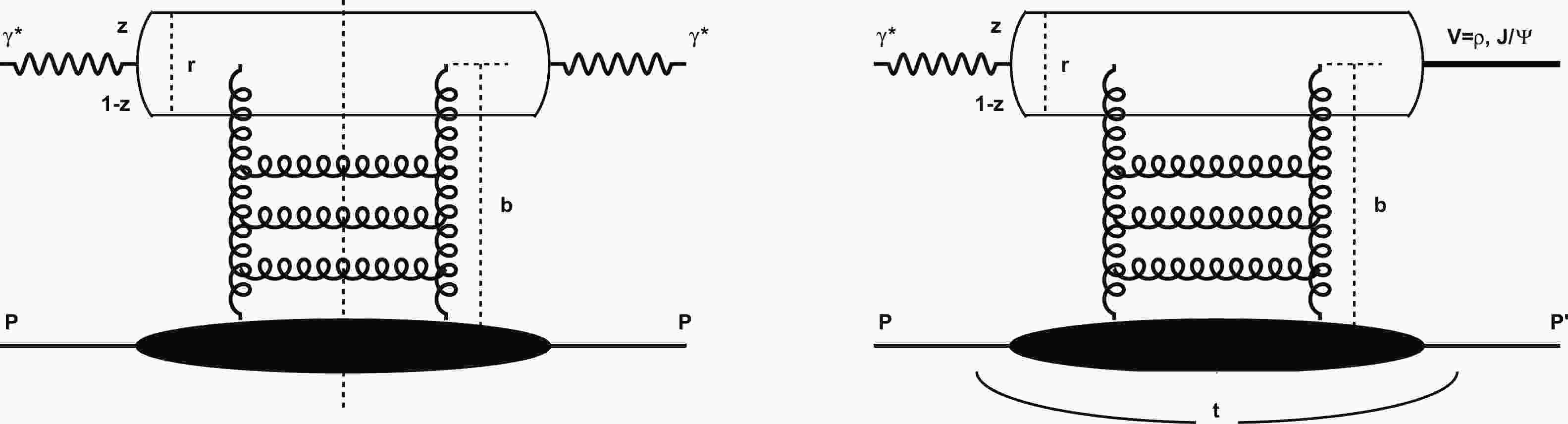
In the proton rest frame, for exclusive vector meson production in the dipole model representation [20, 34, 61], as shown in Fig. 1 (right), even though the momentum transfer
$ {\bf{\Delta}} \neq 0 $ ($ {t}=-{\bf{\Delta}}^{2} $ ), the imaginary part of its amplitude can be similarly expressed as [19]
Figure 1. (left) Elastic scattering amplitude for DIS and (right) amplitude of exclusive vector meson production in dipole model.
$ \begin{aligned}[b] &{\cal{A}}_{\rm T, L}^{\gamma^{*} p \rightarrow V p}(x, Q^{2}, t)= \mathrm{i} \int \mathrm{d}^{2} \boldsymbol{r} \int_{0}^{1} \frac{\mathrm{d} z}{4 \pi} \int \mathrm{d}^{2}\boldsymbol{b}\\ &\times \left(\Psi_{V}^{*} \Psi\right)_{\rm T, L}\left(r,z,Q\right) \mathrm{e}^{-\mathrm{i}[\boldsymbol{b}-(1-z)\boldsymbol{r}]{\bf{\Delta}}}\cdot \frac{ \mathrm{\; d} \sigma_{q \bar{q}}}{\mathrm{\; d}^{2} \boldsymbol{b}}\left(x,r,b\right)\\ =&\mathrm{i} \int_{0}^{\infty} \mathrm{d} r(2 \pi r) \int_{0}^{1} \frac{\mathrm{d} z}{4 \pi} \int_{0}^{\infty} \mathrm{d} b(2 \pi b) \\ &\times\left(\Psi_{V}^{*} \Psi\right)_{\rm T, L} J_{0}(b \Delta) J_{0}([1-z] r \Delta) \frac{\mathrm{d} \sigma_{q \bar{q}}}{\mathrm{\; d}^{2} \boldsymbol{b}}, \end{aligned} $

(1) where
$ \left(\Psi_{V}^{*} \Psi\right)_{\rm T, L} $ is the amplitude of the conversion of a virtual photon into a vector meson.$ { \mathrm{\; d} \sigma_{q \bar{q}}}/{\mathrm{\; d}^{2} \boldsymbol{b}} $ is the dipole scattering differential cross section where$ \boldsymbol{b} $ is the impact parameter. The total dipole-target cross section$ \sigma_{q \bar{q}} $ is obtained by the BK equation.$ J_{0} $ is the first kind of Bessel function. To determine the real part of the amplitude, the ratio of the real to the imaginary parts of the scattering amplitude are used.Thereby, the differential cross section for exclusive vector meson production is given by [14, 16, 20, 21, 61]
$ \frac{\mathrm{d} \sigma_{\rm T, L}^{\gamma^{*} p \rightarrow V p}}{\mathrm{\; d} t}\left(x,Q^2,t \right)=\frac{R^2_g}{16 \pi}\left|{\cal{A}}_{\rm T, L}^{\gamma^{*} p \rightarrow V p}\right|^{2}\left(1+\beta^{2}\right), $

(2) where
$ \beta $ denotes the ratio of the real to the imaginary parts of the scattering amplitude.$ \beta $ is written as$ \beta=\tan (\pi \lambda / 2), \quad {\rm { with }} \quad \lambda \equiv \frac{\partial \ln \left({\cal{A}}_{\rm T, L}^{\gamma^{*} p \rightarrow V p}\right)}{\partial \ln (1 / x)}. $

(3) $ R^2_g $ reflects the skewed effect, given by [62]$ R_{g}=\frac{2^{2 \lambda+3}}{\sqrt{\pi}} \frac{\Gamma(\lambda+5 / 2)}{\Gamma(\lambda+4)}. $

(4) If the dependence of
$ t $ on the amplitude$ {\cal{A}}_{\rm T, L}^{\gamma^{*} p \rightarrow V p} $ is exponential [63], then Eq. (2) is rewritten as$ \frac{\mathrm{d} \sigma_{\rm T, L}^{\gamma^{*} p \rightarrow V p}}{\mathrm{\; d} t}\left(x,Q^2,t \right)=\frac{R^2_g}{16 \pi}\left|{\cal{A}}_{\rm T, L}^{\gamma^{*} p \rightarrow V p}\right|_{t=0}^{2}\left(1+\beta^{2}\right){\rm e}^{-B_{D}|t|}. $

(5) Then, the total cross section is obtained as
$ \sigma_{\rm T, L}^{\gamma^{*} p \rightarrow V p}\left(x,Q^2\right)=\frac{R^2_g}{16\pi B_{D}}\left|{\cal{A}}_{\rm T, L}^{\gamma^{*} p \rightarrow V p}\right|_{t=0}^{2}\left(1+\beta^{2}\right), $

(6) $ \sigma_{\rm tot}^{\gamma^{*} p \rightarrow V p}\left(x,Q^2\right)=\sigma_{\rm T}^{\gamma^{*} p \rightarrow V p}\left(x,Q^2\right)+\sigma_{\rm L}^{\gamma^{*} p \rightarrow V p}\left(x,Q^2\right). $

(7) where
$ B_{D}=N\left(14.0\left(\dfrac{1\; \mathrm{GeV}^{2}}{Q^{2}+M_{V}^{2}}\right)^{0.2}+1\right) $ with$ N=0.55 \;{\rm{GeV}}^{-2} $ for$ \rho^0 $ [63]. For$ J/\psi $ ,$ B_D $ is written as [64, 65]$ B_D= \begin{cases} 4.15+4\times0.116 \ln\left(\dfrac{{W}}{90\;{\rm{GeV}}}\right) &Q^2 \leq 1 \;{\rm{GeV}}^2, \\ 4.72+4\times0.07 \ln\left(\dfrac{{W}}{90\,{\rm{GeV}}}\right) &Q^2 > 1 \;{\rm{GeV}}^2, \end{cases} $

(8) where
$ {W} $ is center of mass energy of$ \gamma^*p $ , which is related to$ x $ and$ Q^2 $ by$ x\,=\,x_{Bj}(1+M^2_V/Q^2)\,=\,\frac{Q^2+M^2_V}{W^2+Q^2}, $

(9) where
$ M_V $ is the mass of the vector meson, and$ x_{Bj} $ is the bjorken scale. For$ J/\psi $ ,$ M_V \,=\,3.097\; {\rm{GeV}} $ , and for$ \rho^0 $ ,$M_V \,=\; 0.776 \;{\rm{GeV}}$ .For overlaps between the photon and vector meson wave functions [19], the transverse and longitudinal polarization parts are
$ \begin{aligned}[b] \left(\Psi_{V}^{*} \Psi\right)_{\rm T}=& \hat{e}_{f} e \frac{N_{\rm c}}{\pi z(1-z)}\left\{m_{f}^{2} K_{0}(\epsilon r) \phi_{\rm T}(r, z)\right.\\ &\left.-\left[z^{2}+(1-z)^{2}\right] \epsilon K_{1}(\epsilon r) \partial_{r} \phi_{\rm T}(r, z)\right\}, \\ \left(\Psi_{V}^{*} \Psi\right)_{\rm L}=& \hat{e}_{f} e \frac{N_{\rm c}}{\pi} 2 Q z(1-z) K_{0}(\epsilon r)\left[M_{V} \phi_{\rm L}(r, z)\right.\\ &\left.+\delta \frac{m_{f}^{2}-\nabla_{r}^{2}}{M_{V} z(1-z)} \phi_{\rm L}(r, z)\right], \end{aligned} $

(10) where
$e = \sqrt{4\pi \alpha_{\rm em}}$ ,$N_{\rm c} = 3$ ,$ \nabla_{r}^{2} \equiv (1 / r) \partial_{r} + \partial_{r}^{2} $ ,$ \epsilon = \sqrt{z(1 - z)Q^2 + m^2_f} $ , Nc = 3 is the number of colors, and the effective charge$ \hat{e}_{f} $ is$ 2/3 $ or$ 1/\sqrt{2} $ for$ J/\psi $ or$ \rho^0 $ , respectively.$ m_f $ is the quark mass.$ K_{0} $ and$ K_{1} $ are the second kind of Bessel function. For the scalar wave functions,$ \phi_{L}(r, z) $ and$ \phi_{T}(r, z) $ , there are two models, "Gaus-LC" [21] and "boosted Gaussian" [61]. It should be noted that we follow the works of other researchers in using$ \delta=0 $ for the "Gaus-LC" model and$ \delta=1 $ for the "boosted Gaussian" model, as mentioned by H. Kowalski et al. [19].For the "Gaus-LC" model, the scalar wave functions,
$ \phi_{L}(r, z) $ and$ \phi_{T}(r, z) $ are written as$ \begin{aligned}[b] \phi_{\rm T}(r, z)=&N_{\rm T}[z(1-z)]^{2} \exp \left(-r^{2} / 2 R_{\rm T}^{2}\right), \\ \phi_{\rm L}(r, z)=&N_{\rm L} z(1-z) \exp \left(-r^{2} / 2 R_{\rm L}^{2}\right). \end{aligned} $

(11) For the "boosted Gaussian" model,
$ \phi_{\rm L}(r, z) $ and$ \phi_{\rm T}(r, z) $ are given by$ \begin{aligned}[b] \phi_{\rm T}(r, z)=& {\cal{N}}_{\rm T} z(1-z) \exp \left(-\frac{m_{f}^{2} {\cal{R}}^{2}}{8 z(1-z)}\right.\left.-\frac{2 z(1-z) r^{2}}{{\cal{R}}^{2}}+\frac{m_{f}^{2} {\cal{R}}^{2}}{2}\right),\\ \phi_{\rm L}(r, z)=& {\cal{N}}_{\rm L} z(1-z) \exp \left(-\frac{m_{f}^{2} {\cal{R}}^{2}}{8 z(1-z)}\right.\left.-\frac{2 z(1-z) r^{2}}{{\cal{R}}^{2}}+\frac{m_{f}^{2} {\cal{R}}^{2}}{2}\right). \end{aligned} $

(12) The parameters in the Eq. (11) and Eq. (12) can be found in [19]. Transverse and longitudinal overlaps between the vector meson functions and the photon function integrated over
$ {z} $ as a function of the dipole size$ {r} $ are presented in Fig. 2.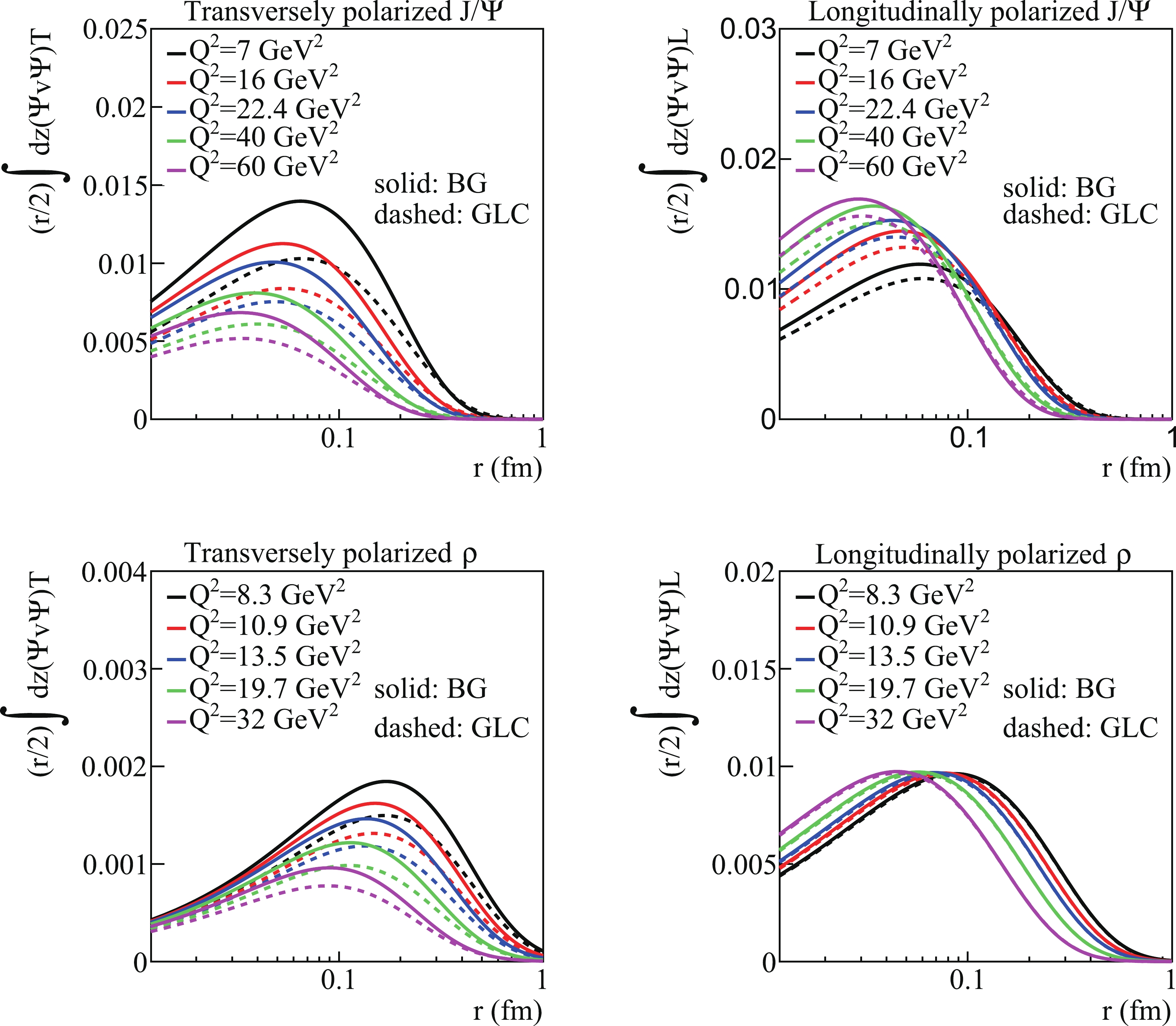
Figure 2. (color online) Transverse and longitudinal overlaps between the vector meson and photon functions as a function of dipole size
$ {r} $ , which are integrated over$ {z} $ . Solid line is for the "Boosted Gaussian" (BG) model, and dashed line is for the "Gaus-LC" (GLC) model.In the following calculations, both models, "Gaus-LC" and "boosted Gaussian," are used. We compare the effects of the two models on the calculation results.
-
In addition to wave functions, the dipole-target scattering amplitude also determines the exclusive vector meson production process. In
$ \left|{\cal{A}}_{\rm T, L}^{\gamma^{*} p \rightarrow V p}\right|_{t=0} $ of Eq. (6), the dipole scattering differential cross section$ \mathrm{d} \sigma_{q \bar{q}}/\mathrm{d}^{2} \boldsymbol{b} $ is integrated and written as$ \int \frac{ \mathrm{\; d} \sigma_{q \bar{q}}}{\mathrm{\; d}^{2} \boldsymbol{b}}(x,r,\boldsymbol{b}) \mathrm{d}^{2} \boldsymbol{b}=\sigma_{q \bar{q}}(x,r)=2\pi R_p^{2}N(x,r), $

(13) where
$ R_p $ is the proton radius, which will be obtained by fitting with the structure function$ F_2 $ data of the proton from the DIS process, and the scattering amplitude$ N(x,r) $ comes from the BK equation.In momentum space, with the proper approximation, the BK equation can be represented as a nonlinear evolution equation [51]
$ \frac{\partial {\cal{N}}({k}, Y)}{\partial Y}= \frac{\alpha_{\mathrm{s}} N_{\mathrm{c}}}{\pi} \chi\left(-\frac{\partial}{\partial \ln {k}^{2}}\right) {\cal{N}}({k}, Y) -\frac{\alpha_{\mathrm{s}} N_{\mathrm{c}}}{\pi} {\cal{N}}^{2}({k}, Y), $

(14) where
$ \chi(\lambda)=\psi(1)-\dfrac{1}{2} \psi\left(1-\dfrac{\lambda}{2}\right)-\dfrac{1}{2} \psi\left(\dfrac{\lambda}{2}\right) $ is the BFKL kernel with$ \psi(\lambda)=\Gamma^{\prime}(\lambda) / \Gamma(\lambda) $ . In addition, αs is a strong coupling constant, and$ Y={\rm ln} $ $ \dfrac{1}{x} $ .When fixing the running strong coupling constant and expanding the BFKL kernel
$ \chi(\lambda) $ [56], we obtain$ A_{0} {\cal{N}}-{\cal{N}}^{2}-\frac{\partial {\cal{N}}}{\partial Y}-A_{1} \frac{\partial {\cal{N}}}{\partial L}+\sum\limits_{p=2}^{P}(-1)^{p} A_{p} \frac{\partial^{p} {\cal{N}}}{\partial^{p} L}=0. $

(15) Here, we need to clarify that the unit of
$ Y $ is$ \bar{\alpha}_{\rm s}=\dfrac{\alpha_{\rm s}N_{\rm c}}{\pi} $ , and$ L={\rm ln}\,k^2/k^2_0 $ . For the calculation, we have fixed$ \bar{\alpha}_{\rm s}=0.191 $ and$ {k}^2_0=\Lambda^{2}_{\rm QCD}=0.04 \; {\rm{GeV}}^2 $ . For$ P=2 $ , the simplified BK equation is given by$ A_{0} {\cal{N}}-{\cal{N}}^{2}-\frac{\partial {\cal{N}}}{\partial Y}-A_{1} \frac{\partial {\cal{N}}}{\partial L}+A_{2} \frac{\partial^{2} {\cal{N}}}{\partial^{2} L}=0. $

(16) The analytical solutions of Eq. (16) have been given as [60]
$ {\cal{N}}( L, Y)=\frac{A_{0} {\rm e}^{5 A_{0} Y / 3}}{\left[{\rm e}^{5 A_{0} Y / 6}+{\rm e}^{\left[-\theta+\sqrt{A_{0} / 6 A_{2}}\left( L- A_{1} Y\right)\right]}\right]^{2}}. $

(17) In this work, the values of
$ A_0 $ ,$ A_1 $ ,$ A_2 $ and$ \theta $ are given by fitting to the proton structure function$ F_2 $ with the following relationship between$ F_2 $ and$ {\cal{N}}(L, Y) $ [66]:$ F_{2}\left(x, Q^{2}\right)=\frac{Q^{2} R_{p}^{2} N_{\rm c}}{4 \pi^{2}} \int_{0}^{\infty} \frac{{\rm d} k}{k} \int_{0}^{1} {\rm d} z \left|\tilde{\Psi}_\gamma\left({k^{2}}, z ; Q^{2}\right)\right|^{2} {\cal{N}}( L, Y), $

(18) where
$ N_{\rm c} $ is the number of colors. Here$ x\,=\,x_{Bj} $ . As shown in Fig. 1 (left), the wave function$ \left|\tilde{\Psi}_\gamma\left({k^{2}}, z; Q^{2}\right)\right|^{2} $ expressed in momentum space represents the probability of a virtual photon splitting into a quark-antiquark pair. It is given by [66]$ \begin{aligned}[b] \left|\tilde{\Psi}_\gamma\left({{k}^{2}}, z ; Q^{2}\right)\right|^{2}= &\sum\limits_{f}\left(\frac{4 \bar{Q}_{f}^{2}}{{{k}^{2}}+4 \bar{Q}_{f}^{2}}\right)^{2} e_{f}^{2}\left.\bigg \{ \left[z^{2}+(1-z)^{2}\right]\right.\\ &\times\left[\frac{4\left({{k}^{2}}+\bar{Q}_{f}^{2}\right)}{\sqrt{{{k}^{2}}\left({{k}^{2}}+4 \bar{Q}_{f}^{2}\right)}} \operatorname{arcsinh}\left(\frac{{{k}}}{2 \bar{Q}_{f}}\right)\right.\\ &\left.+\frac{{{k}^{2}}-2 \bar{Q}_{f}^{2}}{2 \bar{Q}_{f}^{2}}\right]+\frac{4 Q^{2} z^{2}(1-z)^{2}+m_{f}^{2}}{\bar{Q}_{f}^{2}} \\ & \times\left[\frac{{{k}^{2}}+\bar{Q}_{f}^{2}}{\bar{Q}_{f}^{2}}-\frac{4 \bar{Q}_{f}^{4}+2 \bar{Q}_{f}^{2} {{k}^{2}+k^{4}}}{\bar{Q}_{f}^{2} \sqrt{{{k}^{2}}\left({{k}^{2}}+4 \bar{Q}_{f}^{2}\right)}}\right.\\ &\left.\left.\times \operatorname{arcsinh}\left(\frac{{{k}}}{2 \bar{Q}_{f}}\right)\right]\right.\bigg \}, \end{aligned} $

(19) where
$ \bar{Q}_{f}^{2}=z(1-z) Q^{2}+m_{f}^{2} $ , ef and$ m_{f} $ are the charge and the mass of the quark, respectively.In [66], the fitting range for
$ Q^2 $ is$ 0.045 \, \leq Q^{2} \leq 150 \; \mathrm{GeV}^{2} $ , because the corrections from the DGLAP equation should be considered to be in a$ Q^2 $ range that is too high. Therefore, the kinematic fitting range we choose is$ x \, \leq \, 0.01, \quad 1 \, < \, Q^{2} \,\leq \, 45 \; \mathrm{GeV}^{2}. $

(20) The fitting results are presented in Figs. 3, 4. The values of the parameters obtained by fitting to 85
$ F_2 $ data points from H1 and ZEUS [67, 68] with$m_{u,d,s,}\,= \, 0.14\;{\rm{ GeV}} $ and$ m_c\,=\,1.4\;{\rm{GeV}} $ are listed in Table 1.$ \chi^2 $ is also provided in Table 1.$ x $ 

$ Q^2/{\rm{GeV}}^{2} $ 

$ m_{u,d,s}/\,\rm GeV $ 

$ m_{c}/\,\rm GeV $ 

$ \alpha_s $ 

${k }_0/\;\rm GeV$ 

$A_0$ 

$A_1$ 

$A_2$ 

$ \theta $ 

$ R_p/\,\rm GeV^{-1} $ 

$ \chi^2/{\rm nop} $ 

$ \leq\,0.01 $ 

$ (1,45] $ 

0.14 1.4 0.2 0.2 $ 0.696\,\pm\,0.0187 $ 

$ 0.661\,\pm\,0.0295 $ 

$ 0.112\,\pm\,8.0\times10^{-3} $ 

$ -0.463\,\pm\,0.0493 $ 

$ 5.484\,\pm\,0.106 $ 

0.979 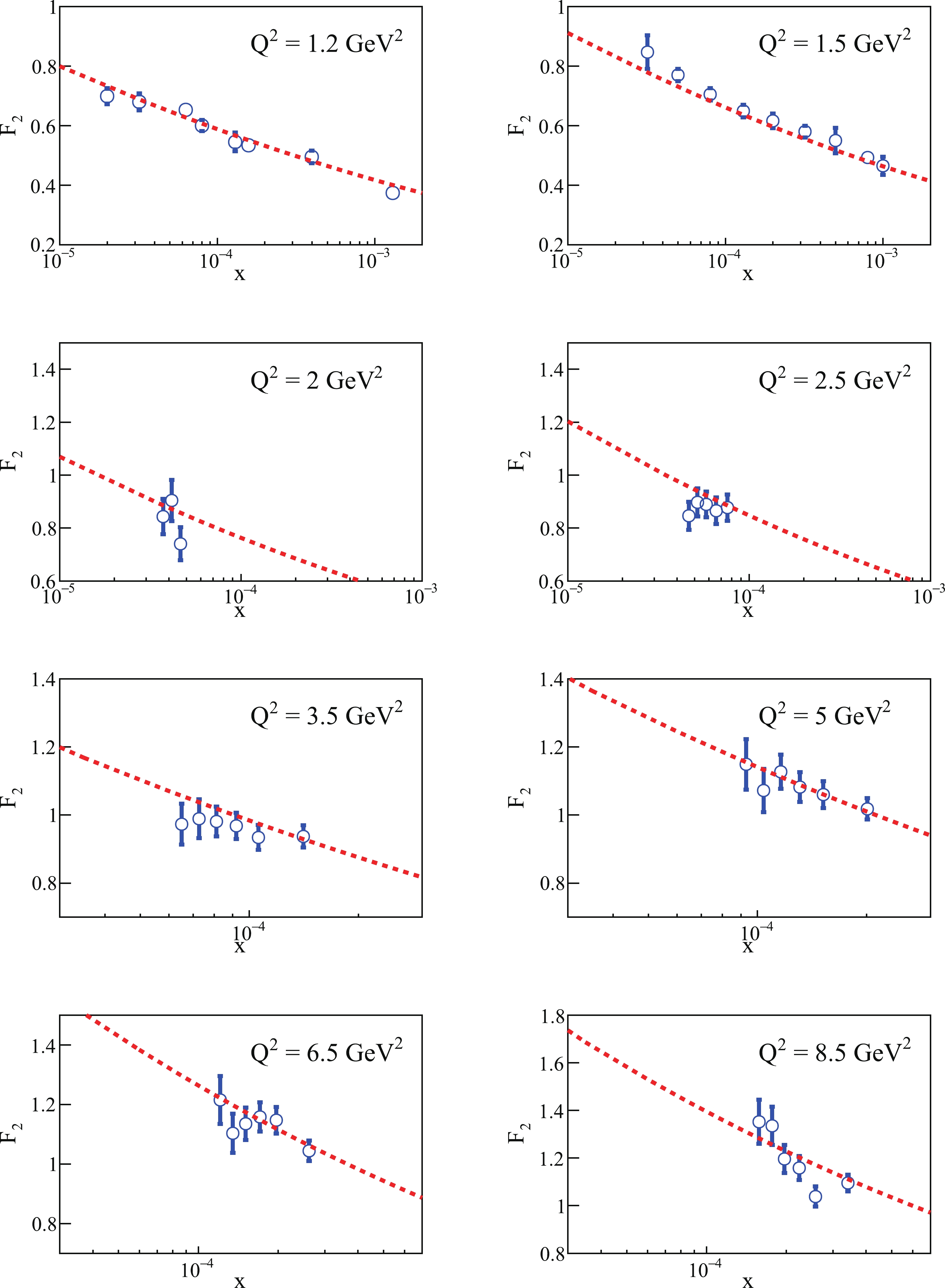
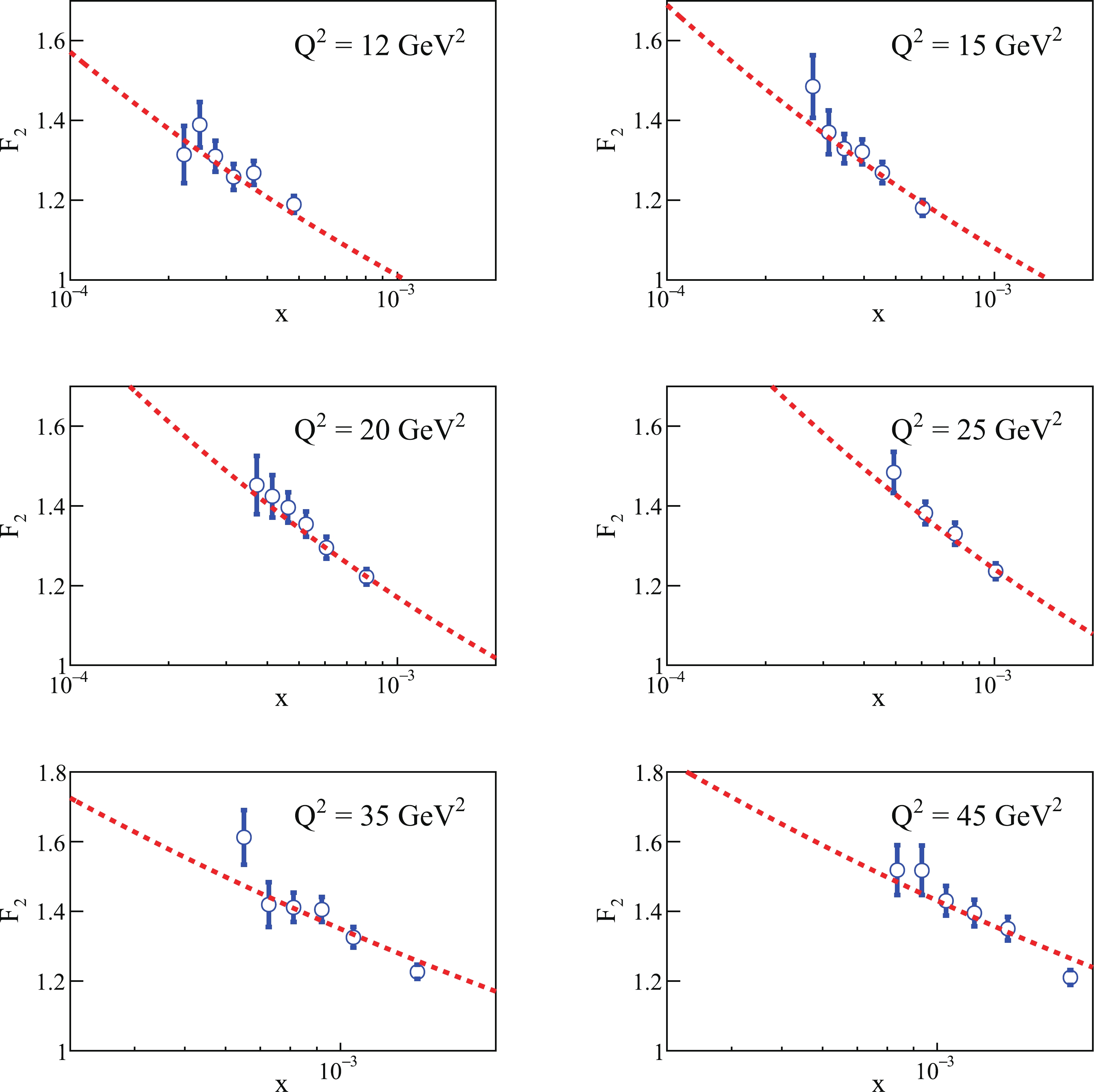
Figure 4. (color online) Continuation of Fig. 3.
Then, in the following calculation, we need the dipole scattering amplitude
$ {\cal{N}}(x,\boldsymbol{r}) $ in the coordinate space.$ {\cal{N}}(x,\boldsymbol{r}) $ is related to$ {\cal{N}}(x,\boldsymbol{k}) $ by the Fourier transformation,$ {\cal{N}}(x,\boldsymbol{k}) = \frac{1}{2\pi}\int\frac{{\rm d}^2\boldsymbol{r}}{r^2}{\rm e}^{{\rm i}\boldsymbol{k}\cdot\boldsymbol{r}}{\cal{N}}(x,\boldsymbol{r}). $

(21) By inverse Fourier transformation, we can get
$ \begin{aligned}[b] {\cal{N}}(x,\boldsymbol{r}) = \frac{r^2}{2\pi}\int{{\rm d}^2\boldsymbol{k}}{\rm e}^{-{\rm i} {k}\cdot\boldsymbol{r}}{\cal{N}}(x,\boldsymbol{k}) =r^2\int^{\infty}_{0}{\rm d}kkJ_0(k\cdot r){\cal{N}}(x,k). \end{aligned} $

(22) Then, we apply Eq. (22) to the total cross section calculations of the
$ J/\psi $ and$ \rho^0 $ productions. -
The cross sections of the vector mesons are calculated with the dipole-amplitude and overlaps between the vector meson and the photon wave functions. In this work, the wave functions of vector mesons adopted are according to two models. The solution of the BK equation shown in the previous section is employed for the dipole-amplitude. We examine whether the solution of the BK equation is valid in these calculations.
We present the differential cross sections, total cross sections and ratios of
$ \sigma_{\rm L} $ and$ \sigma_{\rm T} $ of the$ \rho^0 $ and$ J/\psi $ productions, respectively, using our analytic solution of the BK equation. For the wave functions of the total cross section, we consider the influence of the "Gaus-LC" model and "boosted Gaussian" model. Finally, the total cross sections are calculated theoretically and compared with the experimental data.First of all, the results of the differential cross sections of the
$ J/\psi $ and$ \rho^0 $ productions as a function of t are presented compared with experiment data [69–72], as shown in Fig. 5. Then, we predict the$ {W} $ -dependence total cross sections of two mesons in two wave functions models with our solutions of the BK equation. As shown in Fig. 6, for exclusive$ J/\psi $ and$ \rho^0 $ productions, we compare our results with the experimental data [69–71, 73], in the case of$ 7.0 \leq Q^2\leq22.4 \;{\rm{GeV}}^2 $ and$ 8.3 \leq Q^2 \leq 32.0 \;{\rm{GeV}}^2 $ . From the results, the calculations are reasonable within the range of uncertainty allowed. Moreover, we can find the results obtained by the "Gaus-LC" model and the "boosted Gaussian" model approaching each other as$ Q^2 $ increases. For$ J/\psi $ , the total cross sections obtained by the two models are even flipped-over at higher$ Q^2 $ . This is mainly a contribution from the wave functions. As shown in Fig. 2, for the transversely polarized part of$ \rho^0 $ and$ J/\psi $ , the difference between the two models is gradually reduced as$ Q^2 $ increases. For the longitudinally polarized part of$ \rho^0 $ , the two models are basically the same. However, for$ J/\psi $ , there are some differences between the two models.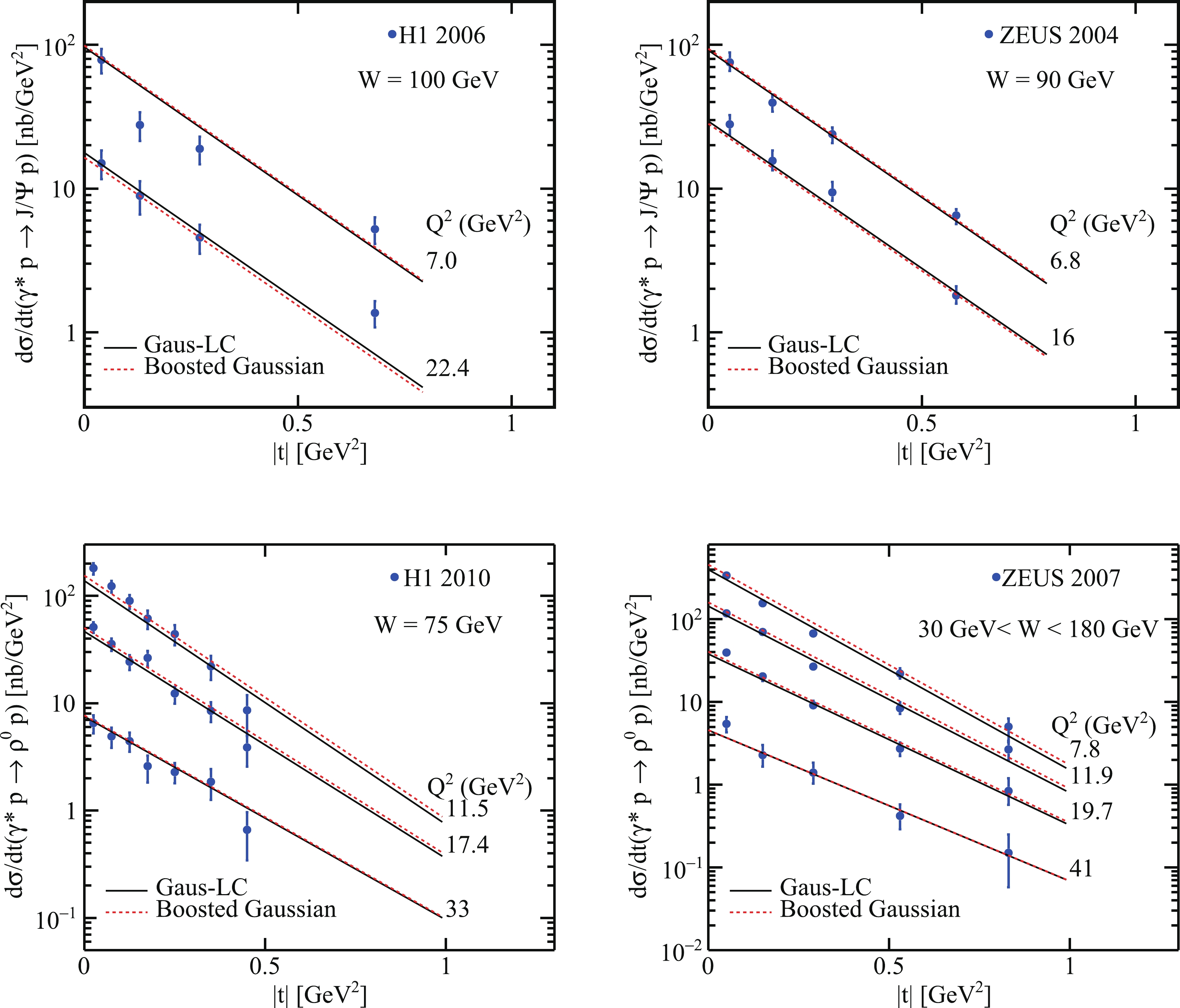
Figure 5. (color online) (above) Calculations of differential cross section of
$\gamma^{*}p \rightarrow J/\psi p$ as a function of$ |{t}| $ compared with experimental data from ZEUS 2004 [69] and H1 2005 [70] using two different meson wave functions. (bottom) Prediction of differential cross section of$ \gamma^{*}p \rightarrow \rho^0 p $ as a function of$ |{t}| $ compared with experimental data from ZEUS 2007 and H1 2010 [71, 72].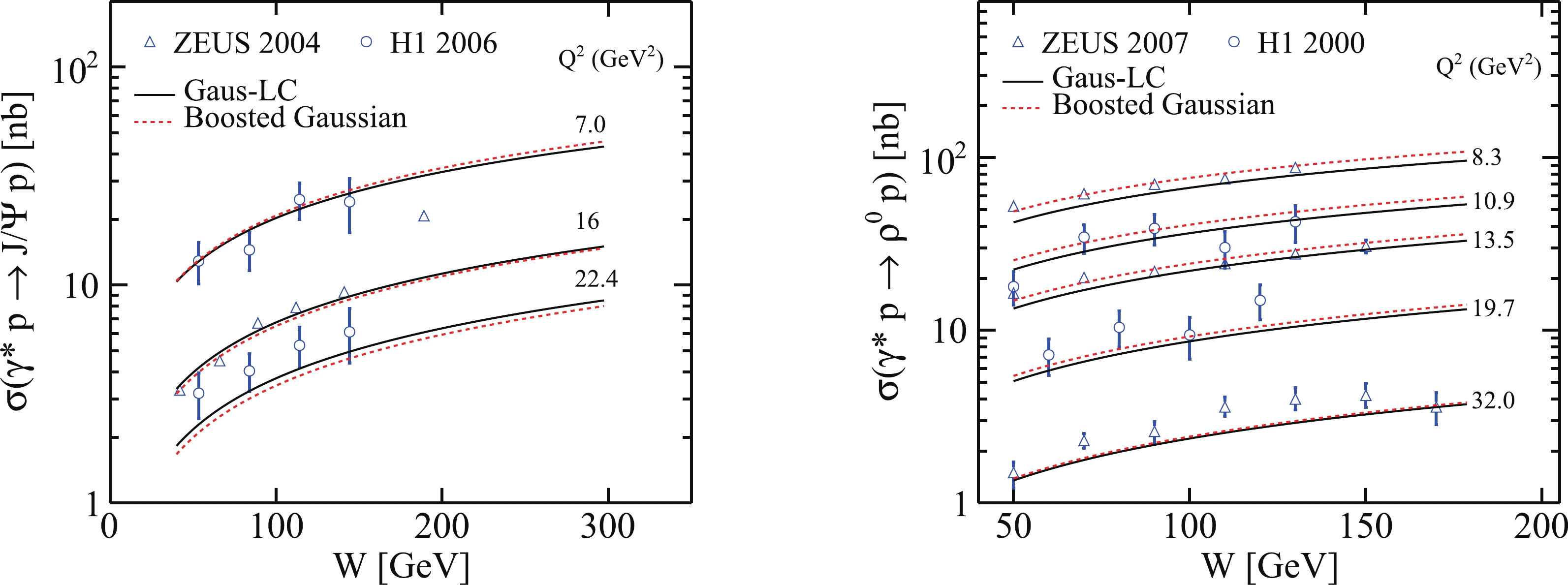
Figure 6. (color online) (left) Prediction of total cross sections of
$\gamma^{*}p \rightarrow J/\psi p$ as a function of$ {W} $ compared with experimental data from ZEUS 2004 [69] and H1 2006 [70] using two different meson wave functions. (right) Prediction of total cross sections of$ \gamma^{*}p \rightarrow \rho^0 p $ as a function of$ {W} $ compared with experimental data from ZEUS 2007 [71] and H1 2000 [73].Secondly, the total cross sections as a function of
$ Q^2 $ are presented in Fig. 7 when$ {W}=90\;{\rm{GeV}} $ for$ J/\psi $ and$ {W}=75\;{\rm{GeV}} $ for$ \rho^0 $ . It can be seen that the predictions agree well with the experimental data. Then, to summarize, the solution of the BK equation is valid for calculations of the cross sections of vector mesons in the diffractive process.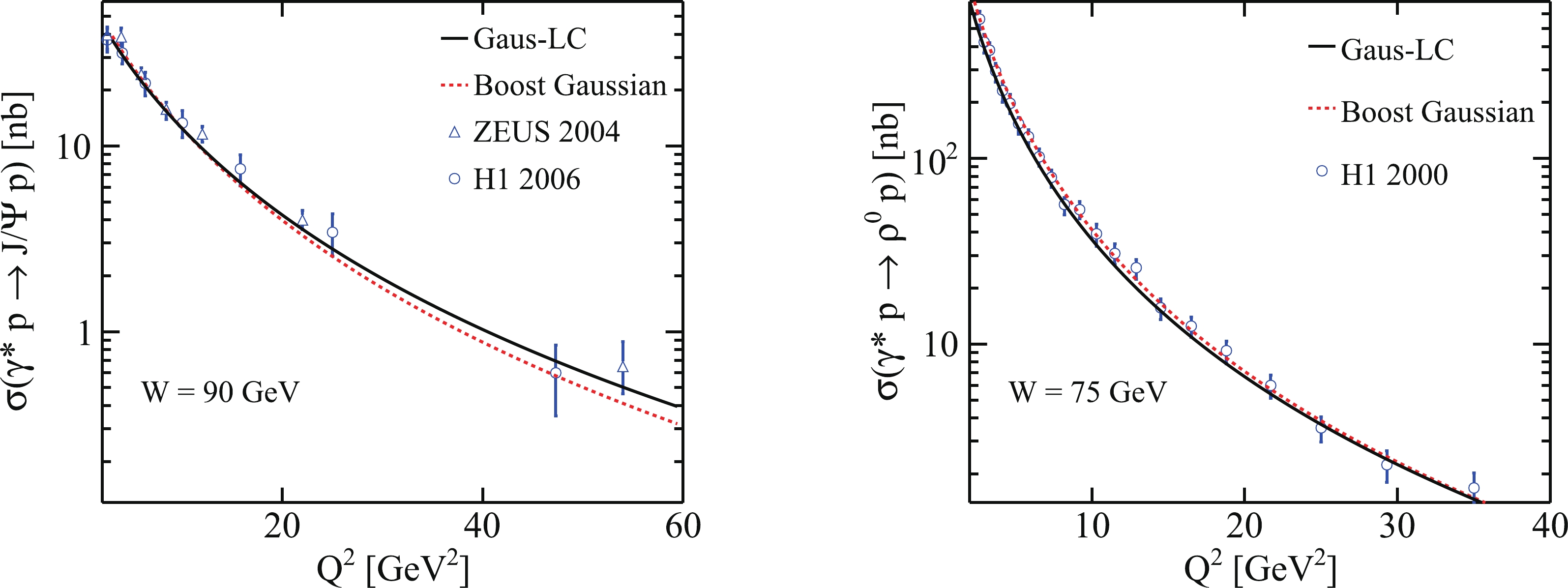
Figure 7. (color online) (left) Prediction for cross sections of
$\gamma^{*}p \rightarrow J/\psi p$ as a function of$ Q^2 $ with two different meson wave functions compared with experimental data from ZEUS 2004 [69] and H1 2006 [70]. (right) Total cross sections of$ \gamma^{*}p \rightarrow \rho^0 p $ as a function of$ Q^2 $ compared with experimental data from H1 2000 [73] using two different meson wave functions.Thirdly, Fig. 8 shows the ratios of the longitudinal to transverse cross section,
$ \sigma_{\rm L}/\sigma_{\rm T} $ , as a function of$ Q^2 $ for fixed$ {\rm{W}} $ . For$ J/\psi $ production,$ \sigma_{\rm L}/\sigma_{\rm T}\,\propto Q^2 $ . Moreover, for the$ \gamma^*p\rightarrow \rho^0 p $ process,$ \sigma_{\rm L}/\sigma_{\rm T} $ based on two wave function models grows rapidly with$ Q^2 $ . As$ Q^2 $ increases, the ratio calculated by us exceeds the experimental data. In [19], a reasonable explanation is given for this situation. The ratios of the longitudinal to transverse cross section are sensitive to the wave functions.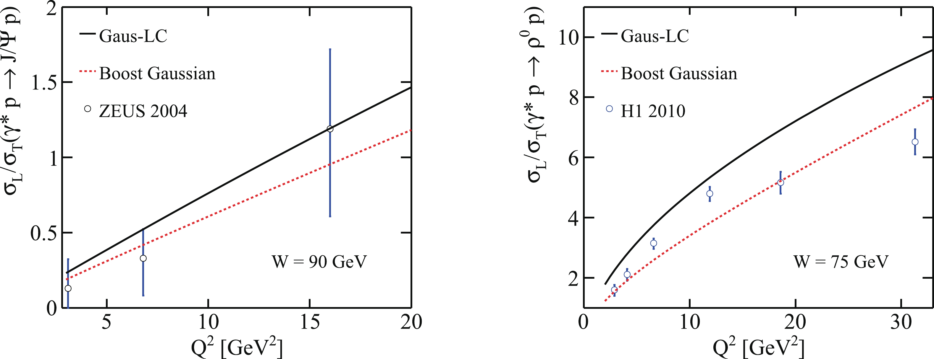
Figure 8. (color online) (left) For
$\gamma^{*}p \rightarrow J/\psi p$ , the ratio of$ \sigma_{\rm L} $ and$ \sigma_{\rm T} $ as a function of$ Q^2 $ with two different meson wave functions compared with experimental data from ZEUS 2004 [69] at$ {\rm{W}}\,=\, 90\;{\rm{GeV}} $ . (right) For$ \gamma^{*}p \rightarrow \rho^0 p $ , the ratio of$ \sigma_{\rm L} $ and$ \sigma_{\rm T} $ as a function of$ Q^2 $ compared with experimental data from H1 2010 [72] using two different meson wave functions at$ {W}= 75\, {\rm{GeV}} $ .Briefly, when the running coupling constant
$ \alpha_s $ is fixed, the solution of the BK equation with the parameters fitted by us in this work is efficient in the prediction of meson production. As$ Q^2 $ increases,$ \alpha_s $ vanishes asymptotically. Only at large$ Q^2 $ , we can assume that its dependence on$ Q^2 $ diminishes. Accordingly, the$ F_2 $ data of$ Q^2\,<\,1\;{\rm{GeV}}^2 $ is not considered. In addition, a very high$ Q^2 $ is also not taken into account, because the DGLAP corrections could work in a region of very high$ Q^2 $ [66]. -
In this work, the good values for the parameters in the solution of the BK equation are obtained by fitting the
$ F_2 $ data first. Then, we use the solution of the BK equation and two wave function models (the "Gaus-LC" model and the "boosted Gaussian" model) to determine the total cross sections of the exclusive$ \rho^0 $ and$ J/\psi $ productions and the ratios of the longitudinal to transverse cross section. The results show that the analytical solution of the BK equation with fixed$ \alpha_{\rm s} $ is suitable for within a certain$ Q^2 $ region. Moreover, the difference between the results caused by the two wave function models decreases with an increase in$ Q^2 $ for$ \rho^0 $ . However, for$ J/\psi $ , at higher$ Q^2 $ , the difference still occurs.To be more precise, our solution of the BK equation with the parameters fitted by us is valid within a region where
$ Q^2 $ is not too high. If this region is exceeded, it may be more appropriate to use the DGLAP equation or the improved BK equation [74, 75].In summary, vector meson production is effective in measuring the properties of protons. In the future, EIC [76] and EicC [77] experimental data will offer more tests of the BK equation.
Exclusive vector meson production with the analytical solution of Balitsky-Kovchegov equation
- Received Date: 2021-12-11
- Available Online: 2022-09-15
Abstract: Exclusive vector meson production is an excellent probe for describing the structure of protons. In this study, based on the dipole model, the differential cross sections, total cross sections, and ratios of the longitudinal to transverse cross section of the


 DownLoad: