


 Abstract
 HTML
HTML Reference
 Related
 PDF
PDF


-
Benefiting from the development of detection technology, cosmic ray physics has entered a precise data-driven era. As we know, secondary cosmic ray particles are produced by primary particles interacting with the interstellar medium (ISM) when they transport in the galaxy. Therefore, the secondary-to-primary ratios reflect the propagation characteristics of cosmic rays. In previous theoretical studies, the cosmic ray propagation paradigm was commonly established using the boron-to-carbon (B/C) ratio [1–5]. However, the importance of other secondary-to-primary ratios, particularly the low-mass ones, has been emphasized in the literature [6–9]. Whether light and heavy nuclei have the same experience in the galaxy is still under debate [8–10]. Recently, antiprotons are suggested to be an important probe in the search for dark matter signals [11–16]. However, if light particles are not accelerated and propagated consistently with the heavy ones, uncertainties may exist in calculating the antiproton background.
To improve our evaluation of cosmic ray physics, we use both the heavy and light nuclei data provided by PAMELA [17], AMS02 [18], ACE-CRIS [19], and Voyager-1 [20] in our analysis. The heavy data used in this paper involve the carbon (C) spectrum and the corresponding secondary-to-primary ratios including the B/C, lithium-to-carbon (Li/C), and beryllium-to-carbon (Be/C) ratios. The low-mass data involve the protons (p) and helium (He) spectra, as well as the corresponding secondary-to-primary ratios such as the antiproton-to-proton (
$ \bar{p}/{p} $ ), the deuteron-to-helium 4 (2H/4He), and the helium 3-to-helium 4 (3He/4He) ratios.Since the AMS02 measurements cover a complex polarity reversal period in the heliospheric magnetic field (HMF), for which the solar effect is difficult to model, we only address AMS02 data [21–26] (including p, He, C,
$ \bar{p}/{p} $ , Li/C, Be/C, B/C) with energies larger than 20 GeV/n. However, no cut is performed on the PAMELA data [27–30] (including p, He, C,$ \bar{p}/{p} $ , 2H/4He, 3He/4He, B/C), since the PAMELA data were collected during a solar minimum period from 2006 to 2008, and the solar modulation during this period is simpler and easier to describe. We also employ the low-energy B/C and C data measured by ACE-CRIS① during the same observational time of PAMELA. Moreover, the energy spectra of interstellar cosmic rays observed by Voyager-1 [31] are included to aid us in further determining the validity of the studied models. With these high-precision data, we aim to study the cosmic ray acceleration and propagation mechanisms more comprehensively and to investigate whether heavy and light nuclei yield compatible results. -
Galactic cosmic rays are frequently considered to be generated from supernova remnants and be accelerated at the expanding supernova shell via the diffusive shock acceleration. They are then ejected into surrounding interstellar gas. For a certain type i of particles, the source abundance can be expressed as
$ {q_i} = \left\{ {\begin{array}{l} {{N_i}f(R){\rho ^{ - {\nu _{1i}}}},}\quad {\rho < {\rho _{bri}}}\\ {{N_i}f(R){\rho ^{ - {\nu _{2i}}}},}\quad {\rho \ge {\rho _{bri}}} \end{array}} \right., $

(1) where R is the radial radius,
$ f \left(R\right) $ is the source spatial distribution in the galaxy,$ N_{i} $ is the normalization abundance of the cosmic ray species i, and ρ is the rigidity of the particle. Different injection indices$ \nu_{1i} $ and$ \nu_{2i} $ above and below a reference rigidity$ \rho_{bri} $ are assumed. In our previous study [8], we assumed that the injection indices for helium nuclei were correlated with those for protons. In contrast, here we permit independent injection indices for different species to determine the actual patterns of source parameters. In this research, we use the cosmic ray propagation software GALPROP v54② [32–35] to calculate the cosmic ray interstellar spectra. The normalization abundances of all other primary species are set relative to the source abundance of protons$ N_{p} $ . Therefore, for species such as He and C, their normalization abundances can be expressed as$ N_{i} = X_{i}N_{p} $ , where$ X_{i} $ is the ratio of the normalized abundance of a certain species i of particles to that of protons. The source radial distribution is assumed to be$ f (R) = (R /R_{\odot})^{\alpha} {\rm e}^{-\beta (R-R_{\odot}} ) $ , where$ R_{\odot} = 8.5 $ kpc. In this study, we set$ \alpha = 0.475 $ and$ \beta = 1.166 $ .After entering the interstellar space, the cosmic rays are influenced by the irregular magnetic field and are scattered randomly in the galaxy. The diffusion coefficient is assumed to be
$ D_{xx} = \left\{ {\begin{array}{l} {D_{0}\beta^{\eta} \left(\dfrac{\rho}{\rho_{0}}\right)^{\delta} ,} \quad {\rho< \rho_{1}} \\ { D_{0}\beta^{\eta} \left(\dfrac{\rho_{1}}{\rho_{0}}\right)^{\delta} \left(\dfrac{\rho}{\rho_{1}}\right)^{\delta_{3}} , } \quad {\rho\geq \rho_{1}} \end{array}} \right. , $

(2) where
$ \beta = \upsilon/c $ is the particle velocity,$ D_{0} $ is the normalization of the diffusion coefficient at a reference rigidity$ \rho_{0} $ , η is a low-energy dependence factor that may be related to the magnetohydrodynamic turbulence dissipation effect [36], and δ is the diffusion slope at rigidities below$ \rho_{1} $ . At rigidities above$ \rho_{1} $ , we introduce a high-energy diffusion slope$ \delta_{3} $ consdiering the hardening at a few hundreds GV observed in primary fluxes [21, 22, 25, 28] and a stronger hardening for secondaries [26]. Moreover, for the pure diffusion model, δ must have different values$ \delta_{1} $ and$ \delta_{2} $ below and above$ \rho_{0} $ [8, 9, 37–39].In addition to diffusion in position space, diffusion may also occur in momentum space owing to the interaction between cosmic rays and magnetic turbulence. As a result, cosmic ray particles may be reaccelerated. The associated diffusion coefficient in momentum space
$ D_{pp} $ is correlated with the spatial diffusion coefficient$ D_{xx} $ as follows:$ D_{pp} = \frac{4v_{A}^{2}p^{2}}{3\delta\left(4-\delta^{2}\right)\left(4-\delta\right)D_{xx}}, $

(3) where
$ v_{A} $ is the Alfvén velocity, corresponding to the turbulence velocity in the hydrodynamical plasma. The magnitude of$ v_{A} $ represents the strength of the reacceleration effect. For the diffusion reacceleration model, a low-energy break on the diffusion slope is not required, i.e.$ \delta_{2} = \delta_{1} $ . Moreover, cosmic rays may also suffer a convection process that transports particles from a galactic disk to a galactic halo. Various assumptions are provided in the literature. For example, a constant convection velocity was assumed in [12, 13], and a linear velocity was adopted in [15, 40]. In this paper, we do not consdier the convection process, but we will further study this mechanism in our future research.After cosmic rays enter the solar system from interstellar space, they are modulated by the solar wind. In this paper, we use force-field approximation [41] to describe the heliospheric modulation. This model can generally describe the periodic data collected during the solar minimum period [42]. For a nucleus with charge Z, mass m, and atomic number A, the modulated cosmic ray energy spectrum at the top of atmosphere
$ J_{\rm{TOA}} $ and the unmodulated interstellar flux$ J_{\rm{IS}} $ are related as follows:$ J_{\rm{TOA}}\left( E \right) = \frac{\left( E+m \right)^2-m^2}{\left(E+m+\dfrac{\left|Z\right|}{A}\phi\right)^2-m^2}J_{\rm{IS}}\left( E+\frac{\left|Z\right|}{A}\phi \right), $

(4) where E is the kinetic energy of the nucleus, and ϕ is the modulation potential.
In summary, the parameters describing the cosmic ray acceleration and propagation mechanisms include the source, propagation, and solar modulation parameters. The source parameters include
$ \nu_{1{p}} $ ,$ \nu_{2{p}} $ ,$ \rho_{br{p}} $ ,$ N_{p} $ ,$ \nu_{1{\rm{He}}} $ ,$ \nu_{2{\rm{He}}} $ ,$ \rho_{br{\rm{He}}} $ , and$ X_{{\rm{He}}} $ for the light nuclei with charge number$ Z\leq2 $ , and$ \nu_{1{\rm{C}}} $ ,$ \nu_{2{\rm{C}}} $ ,$ \rho_{br{\rm{C}}} $ , and$ X_{{\rm{C}}} $ for the heavy nuclei with charge number$ Z>2 $ . The propagation parameters incude$ D_{0} $ ,$ \delta_{1} $ ,$ \delta_{2} $ ,$ \delta_{3} $ ,$ \rho_{0} $ ,$ \rho_{1} $ , η, and$ v_{A} $ . The solar modulation parameter contains only a single parameter ϕ. Since the degeneracy between$ D_{0} $ and the halo size of the galaxy$ z_{h} $ can only be broken by radioactive species, we set$ z_{h} = 4 $ kpc for consistency with earlier studies [8, 40, 43, 44]. However, note that the error estimation of other parameters may be underestimated since$ z_{h} $ is fixed. It is also important to note that the GALPROP resolution parameters influence the accuracy of the calculation. To compromise between calculation speed and accuracy, we set the GALPROP spatial, energy, and time resolution parameters as the values given in Table 1.Resolution parameter Explanation Value $dr$ 

radial grid size 1.0 kpc $dz$ 

height grid size 0.2 kpc $Ekin\_factor$ 

kinetic energy spacing on a logarithmic scale 1.3 $timestep\_factor$ 

scaling factor for timestep reducing 0.25 $start\_timestep$ 

initial timestep $10^{9}$ s

$end\_timestep$ 

final timestep $10^{2}$ s

$timestep\_repeat$ 

timestep repetitions for each timestep_factor 20 Table 1. Numerical scheme parameters of GALPROP adopted in this study.
-
To analyse the experimental data, we use the
$ \chi^{2} $ minimization method in this paper. Compared with the Bayesian analysis, this method requires less computation time and can efficiently estimate the best-fit parameters. It also provides the goodness of fit of each model, i.e., the minimum$ \chi^{2} $ value. Specifically, we interface the minimization library MINUIT [45] with GALPROP to implement the parameter estimation. For each given parameter, the MINUIT processor MINOS is used to reliably calculate its asymmetric errors. The positive and negative MINOS errors are defined as the changes in the value of that parameter that causes the minimum$ \chi^{2} $ value to increase by 1. To achieve accurate estimations of best-fit parameters and their errors, nearly O(104) GALPROP runs are required. For heavy nuclei, the nuclear network begins at 28Si, and the heavy element scan requires nearly 1.4 CPU min per run. For light elements, the nuclear chain begins at 4He, and the scan requires approximately 22 s per run.Fittings are performed using the
$ Z>2 $ and$ Z\leq2 $ nuclei separately. To accurately describe the secondary component of antiprotons, we employ the updated cross-section data provided by [46] and embed a code from [47, 48] in GALPROP to calculate the antiproton productions. For 2H and 3He, based on the cross-sections derived from [6], we modify the corresponding data in the GALPROP file ''eval_iso_cs.dat'' to better determine the productions of 2H and 3He. Some studies observed a possible existence of primary Li [40] or uncertainties on the Li production cross-section [9, 39]. To account for these effects, we introduce a scaling factor on the Li production, i.e.,$ S_ {\rm{Li}} $ . Two different propagation frameworks are studied in this paper: (1) the PDbr model: the plain diffusion model with a low-energy break at a few GV in the diffusion slope, i.e.,$ \delta_{1}\neq \delta_{2} $ ; (2) the DR model: the diffusion-reacceleration model without a low-energy break in the diffusion slope, i.e.,$ \delta_{1} = \delta_{2} $ . -
We first investigate the PDbr and DR models by utilizing a dataset combination with the B/C and C data. The corresponding models are defined as the reference models for heavy particles and are suffixed with "-H0." Since Li and Be, like B, are the secondaries produced by C interacting with the ISM, we further include the accurate AMS02 Li/C and Be/C data in the analysis to check whether they provide compatible results with those derived from only the B/C and C data. When the (Li, Be, B)/C and C data are all included to run the fitting, the corresponding models are suffixed with "-H." Since the normalization abundance of C is calculated according to the abundance of protons, the injection parameters for protons may have an impact on the source term of C. Therefore, when we analyze C and its secondaries, the proton source parameters are fixed at the best-fit values derived from all the light particles, which are detailed in Table 2. By fitting the heavy elements, the estimated source and propagation parameters and the minimized
$ \chi^2 $ value for each model are shown in Table 3.Parameter PDbr-L0 DR-L0 PDbr-L DR-L D0 /(1028cm2 s−1) $3.96\pm^{0.13}_{0.12}$ 

$3.47\pm0.08$ 

$3.76\pm^{0.07}_{0.08}$ 

$4.10\pm0.08$ 

$\delta_{1}$ 

$-0.09\pm0.05$ 

$0.462\pm0.010$ 

$-0.23\pm^{0.04}_{0.05}$ 

$0.386\pm0.009$ 

$\delta_{2}$ 

$0.410\pm0.013$ 

[ $=\delta_{1}$ ]

$0.409\pm^{0.009}_{0.008}$ 

[ $=\delta_{1}$ ]

$\delta_{3}$ 

$0.256\pm^{0.023}_{0.020}$ 

$0.276\pm^{0.023}_{0.027}$ 

$0.257\pm^{0.020}_{0.019}$ 

$0.226\pm^{0.022}_{0.017}$ 

$\rho_{0}$ /GV

$4.62\pm^{0.25}_{0.17}$ 

[4] $4.07\pm^{0.12}_{0.16}$ 

[4] ρ1 /(102GV) $3.2\pm^{0.3}_{0.4}$ 

$4.2\pm0.4$ 

$3.3\pm^{0.3}_{0.4}$ 

$4.0\pm^{0.3}_{0.6}$ 

η $1.06\pm0.14$ 

$-0.03\pm0.08$ 

$1.10\pm0.10$ 

$-0.20\pm^{0.06}_{0.07}$ 

vA /(km s−1) — $15.8\pm^{0.7}_{0.8}$ 

— $12.6\pm^{1.0}_{1.1}$ 

$\nu_{1p }$ 

$1.543\pm0.026$ 

$1.910\pm0.015$ 

$1.47\pm^{0.04}_{0.05}$ 

$1.781\pm0.016$ 

$\nu_{2p }$ 

$2.418\pm0.013$ 

$2.344\pm0.010$ 

$2.417\pm^{0.008}_{0.010}$ 

$2.419\pm0.008$ 

$\rho_{brp }$ /GV

$1.74\pm^{0.08}_{0.07}$ 

$5.9\pm0.4$ 

$1.40\pm^{0.09}_{0.13}$ 

$3.18\pm^{0.11}_{0.10}$ 

$\nu_{1\text{He}}$ 

$1.439\pm0.021$ 

$1.593\pm0.019$ 

$1.455\pm^{0.023}_{0.019}$ 

$1.492\pm^{0.019}_{0.018}$ 

$\nu_{2\text{He}}$ 

$2.357\pm0.012$ 

$2.280\pm0.009$ 

$2.355\pm^{0.008}_{0.009}$ 

$2.365\pm0.007$ 

$\rho_{br\text{He}}$ /GV

$2.43\pm0.06$ 

$2.45\pm^{0.12}_{0.10}$ 

$2.361\pm^{0.022}_{0.013}$ 

$2.36\pm^{0.04}_{0.02}$ 

Np /(10−9cm−2 sr−1 s−1 MeV−1) $4.317\pm0.012$ 

$4.313\pm0.012$ 

$4.318\pm0.012$ 

$4.323\pm^{0.011}_{0.012}$ 

$X_{\text{He}}$ 

$0.032\pm^{0.004}_{0.003}$ 

$0.60\pm^{0.14}_{0.11}$ 

$0.020\pm^{0.004}_{0.005}$ 

$0.151\pm0.011$ 

ϕ GV $0.423\pm0.007$ 

$0.442\pm^{0.007}_{0.008}$ 

$0.424\pm^{0.007}_{0.008}$ 

$0.441\pm^{0.006}_{0.007}$ 

$\chi^{2}$ /d.o.f

1.76 1.90 1.67 2.15 Table 2. Best-fit parameters for PDbr-L0, DR-L0, PDbr-L, and DR-L models constrained by the Z
$ \leq $ 2 data. The fixed parameters appear in square brackets.Parameter PDbr-H0 DR-H0 PDbr-H DR-H D0 /(1028cm2 s−1) $3.2\pm^{0.4}_{0.3}$ 

$2.18\pm^{0.15}_{0.14}$ 

$3.34\pm^{0.25}_{0.22}$ 

$3.00\pm^{0.23}_{0.22}$ 

$\delta_{1}$ 

$-1.6\pm0.4$ 

$0.435\pm^{0.019}_{0.018}$ 

$-1.4\pm0.4$ 

$0.446\pm0.014$ 

$\delta_{2}$ 

$0.462\pm0.016$ 

[ $=\delta_{1}$ ]

$0.472\pm^{0.013}_{0.012}$ 

[ $=\delta_{1}$ ]

$\delta_{3}$ 

$0.31\pm^{0.03}_{0.04}$ 

$0.26\pm^{0.03}_{0.04}$ 

$0.310\pm^{0.026}_{0.027}$ 

$0.29\pm^{0.03}_{0.04}$ 

ρ0 /GV $3.86\pm^{0.19}_{0.15}$ 

[4] $3.91\pm^{0.20}_{0.15}$ 

[4] ρ1 /(102GV) $2.2\pm^{0.4}_{0.3}$ 

$2.2\pm^{0.5}_{0.3}$ 

$2.1\pm0.4$ 

$2.3\pm^{0.5}_{0.4}$ 

η $2.5\pm0.7$ 

$0.04\pm^{0.19}_{0.20}$ 

$2.2\pm^{0.7}_{0.6}$ 

$-0.27\pm0.17$ 

vA /(km s−1) — $17.6\pm1.0$ 

— $17.2\pm^{1.8}_{1.9}$ 

$\nu_{1\text{C}}$ 

$0.32\pm^{0.14}_{0.15}$ 

$0.68\pm^{0.12}_{0.20}$ 

$0.36\pm^{0.11}_{0.12}$ 

$1.42\pm0.04$ 

$\nu_{2\text{C}}$ 

$2.338\pm0.012$ 

$2.412\pm0.010$ 

$2.328\pm0.010$ 

$2.353\pm^{0.011}_{0.012}$ 

$\rho_{br\text{C}}$ /GV

$1.22\pm^{0.06}_{0.05}$ 

$1.51\pm^{0.09}_{0.12}$ 

$1.22\pm0.04$ 

$2.47\pm0.10$ 

XC (10−3) $3.3\pm^{0.5}_{0.4}$ 

$23\pm^{5}_{3}$ 

$3.12\pm^{0.27}_{0.26}$ 

$5.0\pm^{0.8}_{0.7}$ 

$S_{\text{Li}}$ 

[1] [1] $1.234\pm0.013$ 

$1.243\pm0.013$ 

ϕ /GV $0.442\pm0.014$ 

$0.514\pm^{0.013}_{0.012}$ 

$0.443\pm0.012$ 

$0.409\pm0.013$ 

$\chi^{2}/$ d.o.f

0.92 0.91 0.86 1.45 Table 3. Best-fit parameters for PDbr-H0, DR-H0, PDbr-H, and DR-H models constrained by the
$ Z>2 $ data. The fixed parameters appear in square brackets.We observe that the best-fit parameters of the PDbr-H model are consistent with those of the PDbr-H0 model, with slightly improved accuracies. The best-fit propagation parameters of the DR-H model also agree well with those of the DR-H0 model. However, the best-fit source and solar modulation parameters of the DR-H model, i.e.,
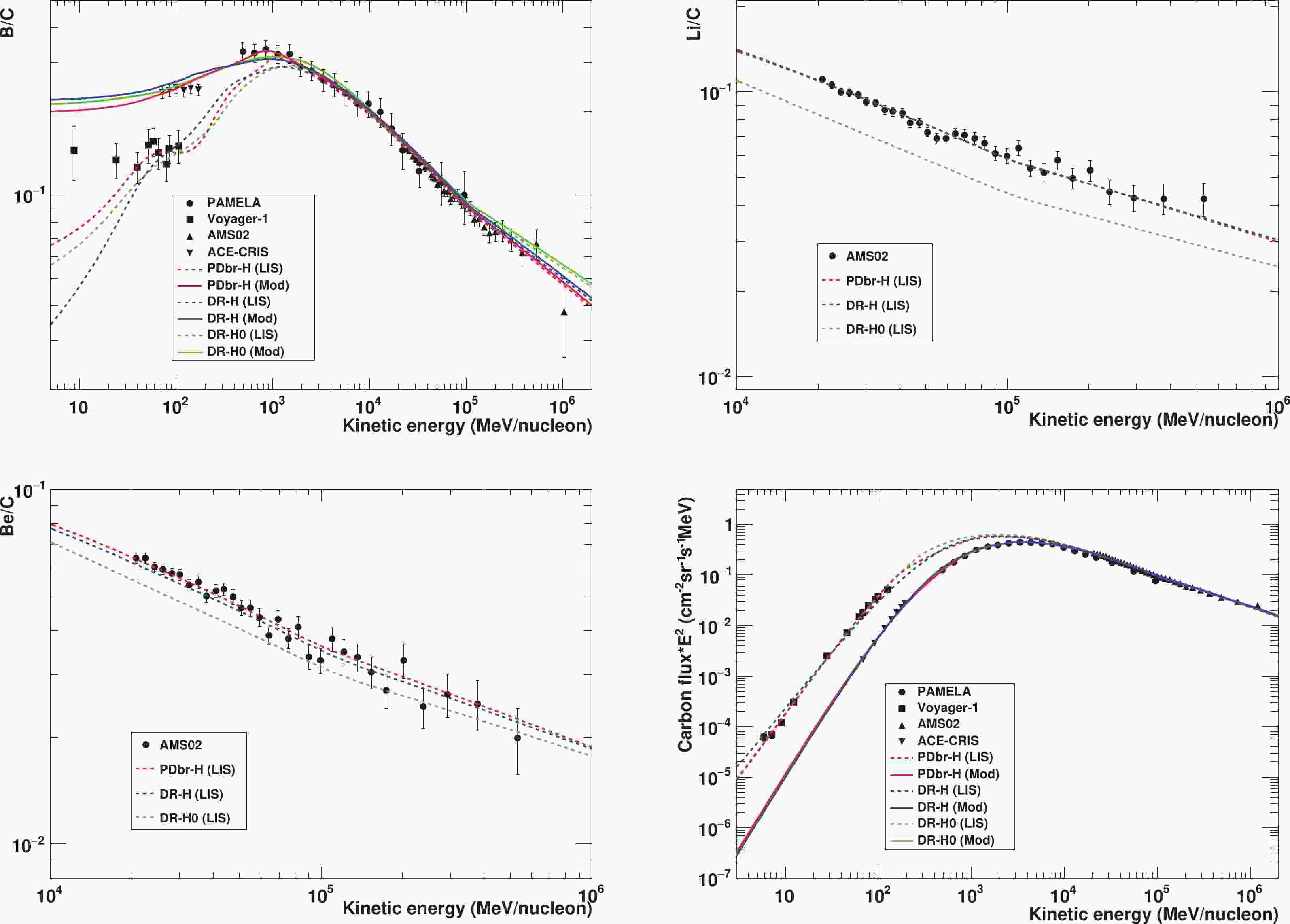
$ \nu_{1{\rm{C}}} $ ,$ \nu_{2{\rm{C}}} $ ,$ X_{{\rm{C}}} $ , and ϕ, differ significantly from those of the DR-H0 model. Moveover, as shown in Fig. 1, the theoretical calculation of Li/C for the DR-H0 model disagrees dramatically with other models and experimental data. This discrepancy of Li may be caused by different values of$ S_{\rm{Li}} $ adopted in the calculation. However, the prediction of Be/C using the DR-H0 model exhibits distinct disagreements with the AMS02 data below 60 GeV/n. This indicates that the use of only the B/C and C data may not provide reliable constraints on the source and transport mechanisms for heavy particles. In the following paragraphs, we focus on discussing the PDbr-H and DR-H models.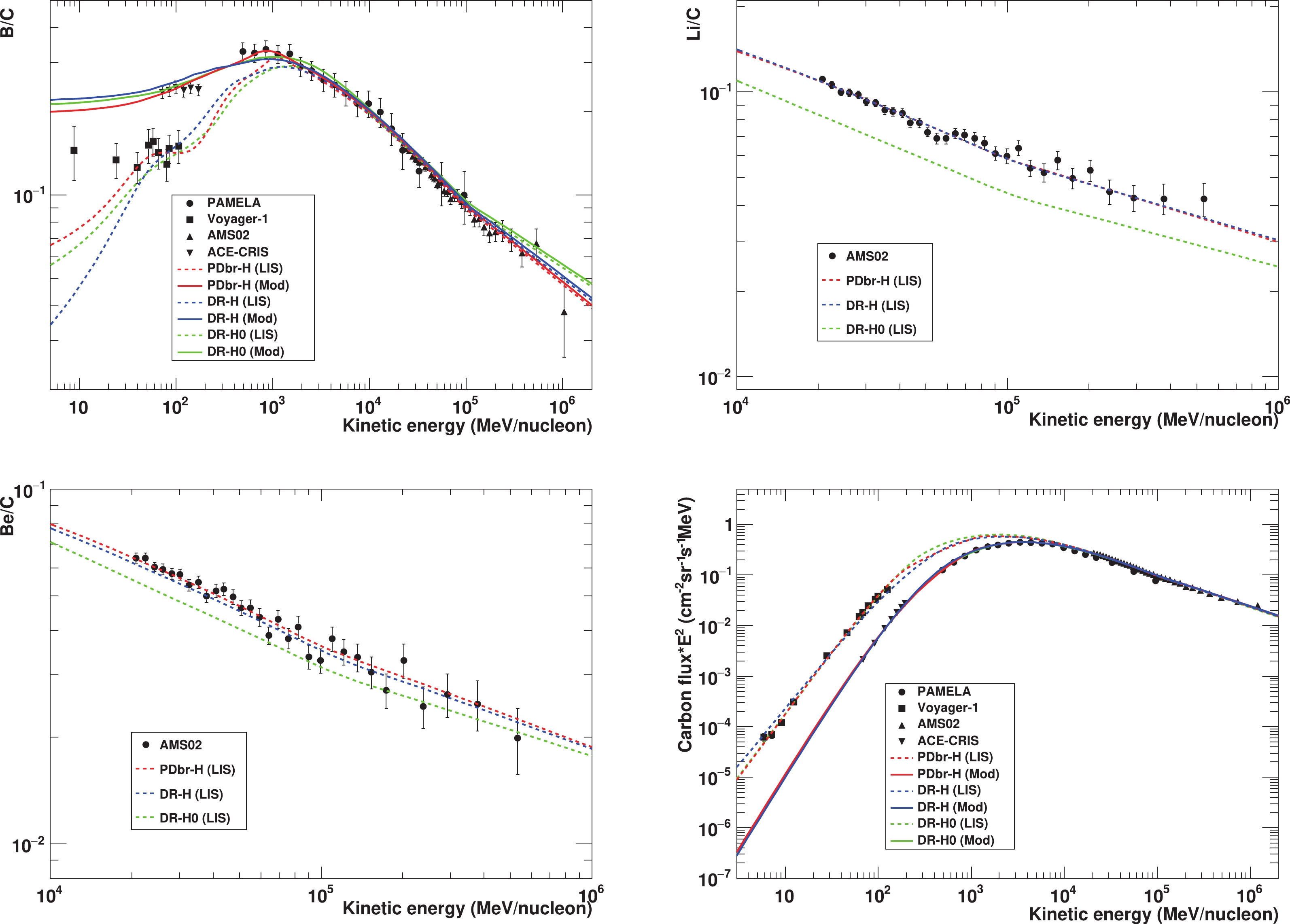
Figure 1. (color online) B/C, Li/C, Be/C ratios and carbon flux for the best-fit parameters of the PDbr-H, DR-H, and DR-H0 models as listed in Table 3. The calculation with the PDbr-H0 model cannot be distinguished with that with PDbr-H and is not shown here. The solid (dashed) lines represent the interstellar (modulated) spectra and ratio. Data points are the measurements from PAMELA, AMS02, ACE-CRIS, and Voyager-1.
For the PDbr-H and DR-H models, the diffusion spectral index
$ \delta_{2} $ are well constrained in$ \left(0.43, 0.48\right) $ . The$ \Delta\delta_{H} = \delta_{3}-\delta_{2} $ values estimated with the PDbr-H and DR-H models are$ -0.16\pm0.03 $ and$ -0.16\pm^{0.04}_{0.05} $ , respectively. These results indicate that a consistent change in the diffusion slope at$ 200\sim300 $ GV exists in both models, which may be responsible for the hardening in primary and secondary cosmic ray spectra above a few hundred GV. Though the high-energy behaviors are explicit, the phenomena at low energies are model-dependent. For example, the estimated η is much smaller when a reacceleration process is considered. Since the Li/C and Be/C data employed in the analysis are those with energies larger than 20 GeV/n, the low-energy propagation parameters are primarily constrained by the B/C data. To explain the B/C peak at 1 GeV/n, either a diffusion slope variation$ \Delta\delta_{L} = \delta_{2}-\delta_{1}\sim1.9\pm0.5 $ at 4 GV or an Alfvén velocity$ v_{A}\sim17.2\pm^{1.8}_{1.9} $ km s-1 is required. However, Fig. 1 shows that both models expect lower ratios than the Voyager-1 data below 20 MeV/n, as already emphasized in [31]. The best-fit values of$ S_ {\rm{Li}} $ are observed to be$ 1.234\pm0.013 $ and$ 1.243\pm0.013 $ in the PDbr-H and DR-H models, respectively. These results can be considered as either a possible signal of primary Li or a hint of an inaccurate cross-section normalization of Li. Nevertheless, both the PDbr-H and DR-H models can generally reproduce all the$ Z>2 $ data. -
To better understand the cosmic ray source and transport phenomena for light elements, we further implement a
$ \chi^{2} $ analysis of the Z$ \leq $ 2 species. Similar with the treatment of heavy particles, we first examine the PDbr and DR models by employing a commonly-used dataset combination with the$ \bar{p}/{p} $ , p, and He data. The corresponding models are suffixed with "-L0." Subsequently, we include the 2H/4He and 3He/4He data in the analyses. The corresponding models are suffixed with "-L." The estimated best-fit parameters and the$ \chi^{2} $ value for each model are presented in Table 2.The best-fit values of
$ \delta_{2} $ are$ 0.410\pm0.013 $ for the PDbr-L0 model and$ 0.462\pm0.010 $ for the DR-L0 model. These two values generally agree with those derived from heavy particles, which indicates that the$ \bar{p}/{p} $ data can yield compatible results of$ \delta_{2} $ with the B/C data. By adding the 2H/4He and 3He/4He ratios in the fitting, the PDbr-L model provides consistent results with the PDbr-L0 model. However, we observe that the DR-L model yields inconsistent parameters compared with the DR-L0 model. For example, the$ \delta_{2} $ value is varied prominently from$ 0.462\pm0.010 $ in the DR-L0 model to$ 0.386\pm0.011 $ in the DR-L model. This is because the DR-L0 model can not reproduce the PAMELA 2H/4He, 3He/4He data below 1 GeV/n, as shown in Fig. 2. Therefore, an inclusion of the 2H/4He and 3He/4He data in the fitting results in different estimations of source and transport parameters in the DR-L model. In the following paragraphs, we focus on discussing the PDbr-L and DR-L models.
Figure 2. (color online)
$ \bar{p}/{p} $ , 2H/4He, 3He/4He ratios and the antiproton, proton, and helium fluxes for the best-fit parameters of the PDbr-L0, PDbr-L, DR-L0, and DR-L models as listed in Table 2. The solid (dashed) lines represent the interstellar (modulated) spectra and ratio. Data points are the measurements from PAMELA, AMS02, and Voyager-1.Under the same configuration, i.e., the PDbr or DR configuration, the value of
$ \delta_{2} $ determined by$ \bar{p} $ , 2H, 3He, p, and He, is about 0.06 lower than that obtained from Li, Be, B, and C. This is also true for$ \delta_{3} $ . However, the$ \Delta\delta_{H} $ values estimated in the PDbr-L and DR-L models remain consistent with those derived in the PDbr-H and DR-H models. It appears that a same level of variation in the diffusion slope at a few hundreds GV can explain the hardening in cosmic ray spectra or ratios for both light and heavy particles. Moreover, since we assume that p and He have the same diffusion slopes, the observational difference between the p and He spectra is explained by the difference between their injection indices. This can be observed in Table 4. For the high-energy injection parameters, the estimated$ \nu_{2{\rm{He}}} $ is lower than the$ \nu_{2{p}} $ value in both the PDbr-L and DR-L models. The$ \nu_{2{\rm{C}}} $ value in the PDbr-H (or DR-H) model is estimated to be lower than the$ \nu_{2{\rm{He}}} $ value obtained in the PDbr-L (or DR-L) model. It appears that above a few GV, the lighter the particle, the larger the injected spectral index.PDbr-L v.s. PDbr-H DR-L v.s. DR-H $\nu_{2p}-\nu_{2\text{He}}$ 

$0.062\pm^{0.012}_{0.014}$ 

$0.054\pm0.011$ 

$\nu_{2\text{He}}-\nu_{2\text{C}}$ 

$0.027\pm^{0.013}_{0.014}$ 

$0.012\pm0.014$ 

$\nu_{1p}-\nu_{1\text{He}}$ 

$0.02\pm^{0.05}_{0.06}$ 

$0.289\pm0.025$ 

$\nu_{1\text{He}}-\nu_{1\text{C}}$ 

$1.10\pm^{0.12}_{0.13}$ 

$0.07\pm0.05$ 

Table 4. Differences in the injection index between various primary cosmic ray species.
At low energies, a diffusion slope variation
$ \Delta\delta_{L} = 0.64\pm^{0.05}_{0.06} $ or an Alfvén velocity$ v_{A} = 12.6\pm^{1.0}_{1.1} $ km s-1 is necessary to reconcile all the light nuclei data. However, while the PDbr-L model agrees well with the$ \bar{p}/{p} $ data, the DR-L model cannot fit the$ \bar{p}/{p} $ data below 1 GeV. This is one reason for the larger$ \chi^{2} $ obtained by DR-L compared with the PDbr-L model. Additionally, we calculate the predictions of the antiproton flux for the PDbr-L and DR-L models, as shown in Fig. 2. We observe that both models can generally reproduce the PAMELA and AMS02 antiproton fluxes. Nevertheless, compared with the heavy nuclei, the low-mass data imply a smaller change in diffusion slope or a weaker reacceleration process. The low-energy injection properties are model-dependent. As shown in Table 4, we obtain$ \nu_{1{p}}\approx\nu_{1{\rm{He}}}>\nu_{1{\rm{C}}} $ for the PDbr configuration but$ \nu_{1{p}}>\nu_{1{\rm{He}}}\approx\nu_{1{\rm{C}}} $ for the DR configuration. Both results are not easy to explain with current knowledge of acceleration mechanisms. Furthermore, as observed in Fig. 2, both the PDbr-L and DR-L models have disagreements with the PAMELA 3He/4He ratio below 300 MeV/n and the PAMELA helium data below 400 MeV/n. This may be because the force-field approximation is based on the zero streaming hypothesis, which is only valid above 400 MeV/n [41]. Additionally, it is worth noting that both the light and heavy elements yield compatible values of ϕ. This strengthens the robustness of the solar effect description for PAMELA data above 400 MeV/n. -
To further understand the differences between light and heavy nuclei, we theoretically calculate the B/C, Li/C, and Be/C ratios based on the propagation and solar modulation parameters estimated in the PDbr-L(0) and DR-L(0) models. The results are presented in Fig. 3. As the figure shows, no model can provide a satisfactory prediction for the B/C ratio. At energies larger than 20 GeV/n, while the DR-L0 model predicts a slightly lower B/C ratio than the AMS02 data, the PDbr-L model predicts a higher ratio than the AMS02 observations. Compared with the DR-L0 and PDbr-L models, the DR-L model is closer to the AMS02 B/C data, but deviates further with the data at a few GeV/n. In the MeV range, only DR-L can fit the ACE-CRIS data. For each model, the prediction features of high-energy Li/C and Be/C ratios are similar to that of the B/C ratio. Nevertheless, none of them can explain the B/C bump at 1 GeV/n. This indicates that compared with the light nuclei, a much larger diffusion slope variation
$ \Delta\delta_{L} $ or a stronger$ v_{A} $ is preferred to interpret the B/C peak.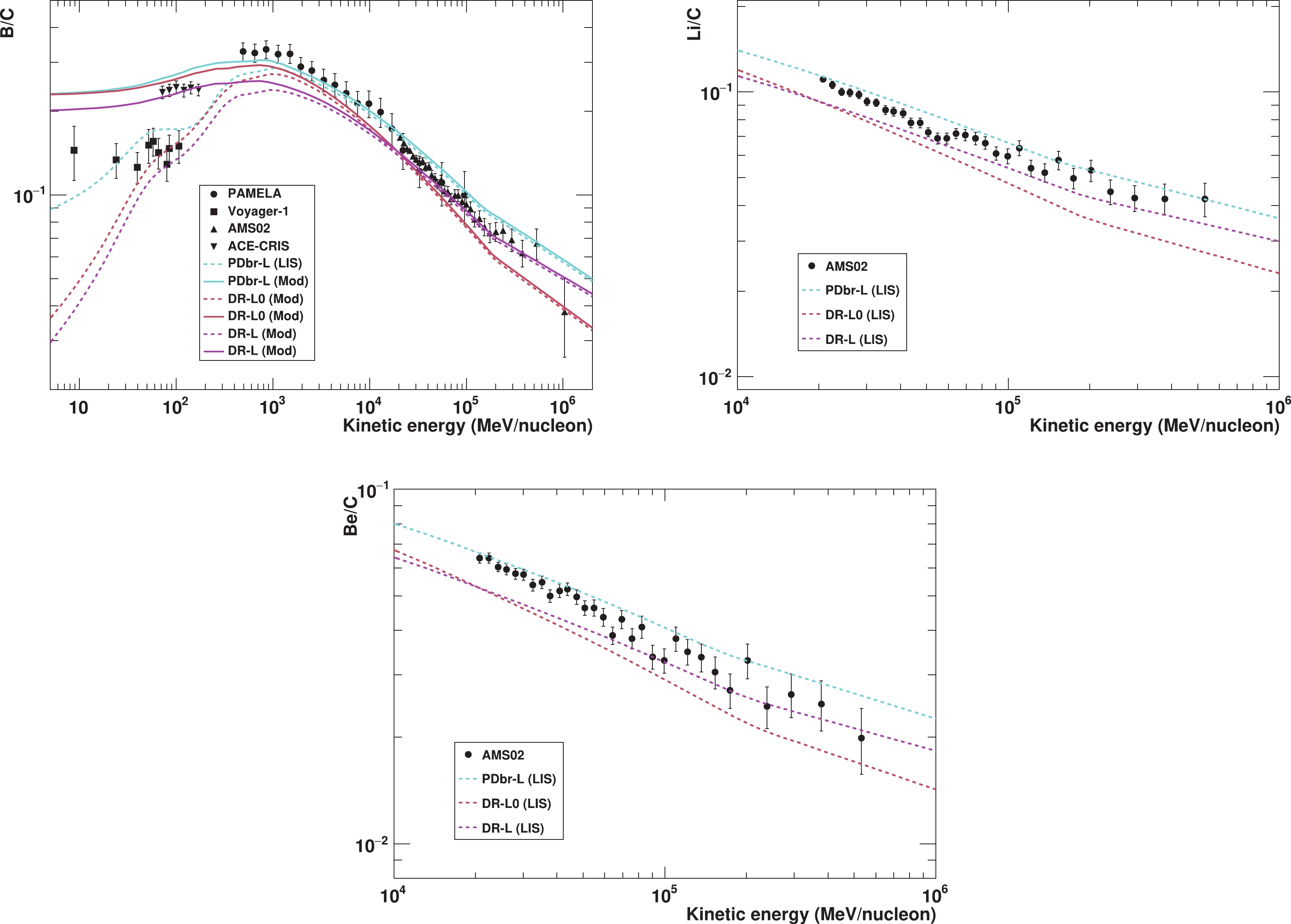
Figure 3. (color online) B/C, Li/C, and Be/C ratios for the best-fit parameters of the PDbr-L, DR-L0, and DR-L models as listed in Table 2. The calculation from the PDbr-L0 model cannot be distinguished with that from PDbr-L and is not shown here. The solid (dashed) lines represent the interstellar (modulated) spectra and ratio. Data points are the measurements from PAMELA, AMS02, ACE-CRIS, and Voyager-1.
Subsequently, we calculate the
$ \bar{p}/{p} $ , 2H/4He, and 3He/4He ratios based on the best-fit parameters estimated in the PDbr-H and DR-H models. As shown in Fig. 4, the PDbr-H model appears to fit$ \bar{p}/{p} $ ratio almost over all the energy range but cannot fit the 2H/4He and 3He/4He data. This demonstrates that the PDbr-H model can accommodate both the light and heavy nuclei above 1 GeV/n. This also indicates that we may be able to use the parameters derived from the heavy nuclei to predict antiprotons above 1 GeV/n. A clear distinction appears between the DR-H model and the$ \bar{p}/{p} $ data above 10 GeV. Furthermore, both the PDbr-H and DR-H models do not agree with the PAMELA 2H/4He and 3He/4He ratios, which further implies the possible incompatibilities between the models and the low-energy light elements. Some studies attributed the discrepancies to uncertainties in solar modulation and (or) the antiproton cross-sections [11, 15], and correlations in data systematic errors [4, 9, 49, 50]. These impacts are further discussed in Sec. III.D.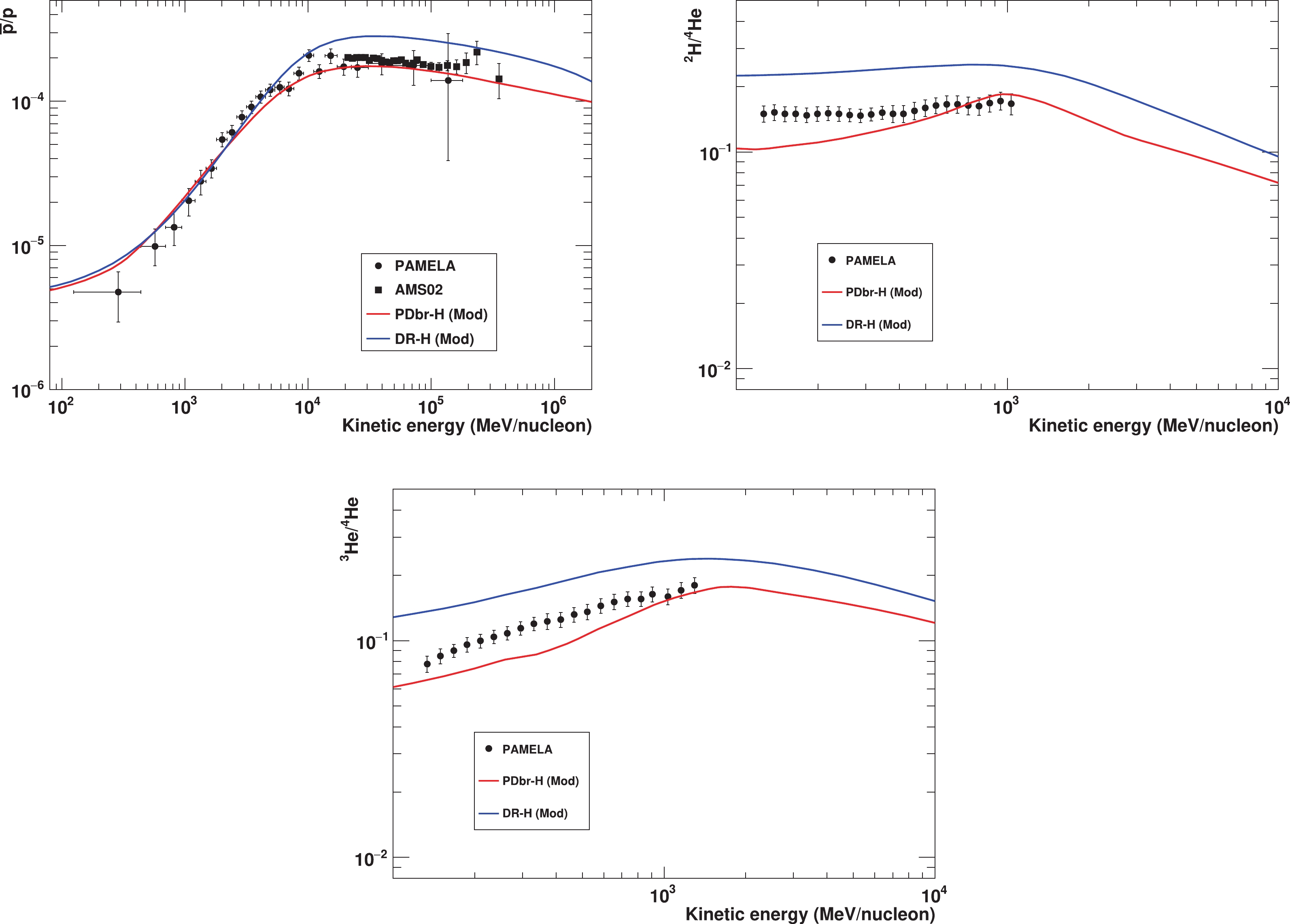
Figure 4. (color online)
$ \bar{p}/{p} $ , 2H/4He and 3He/4He ratios for the best-fit parameters of the PDbr-H and DR-H models as listed in Table 3. Data points are the measurements from PAMELA, AMS02, and Voyager-1. -
Compared with our previous study [8], in which we fitted only the PAMELA 2H/4He, 3He/4He, p, and He data and the Voyager-1 p and He interstellar spectra, this updated study fits a more complete low-mass data by including the
$ \bar{p}/{p} $ data and high-energy AMS02 p and He data while performing a separate analysis of the (Li, Be, B)/C, and C data. When we considered different configurations, the high-energy diffusion slope$ \delta_{2} $ obtained in [8] varied significantly (from 0.2 to 0.8), but in this paper, we achieve a much more accurate estimation of$ \delta_{2} $ between 0.38 and 0.48. This is because the 2H/4He and 3He/4He ratios used in the previous paper were only in the MeV to GeV range and could not place strong constraints on the high energy propagation behavior. Moveover, a different choice of solar modulation model may affect our evaluations of$ \delta_{2} $ . In our previous study, we adopted a rigidity and charge-sign dependent solar modulation (CM) model [51]; however, we observe that the CM model cannot accommodate ACE-CRIS B/C and C data in the MeV range and is not incorporated in this paper.It is interesting to compare our results with some studies. The analysis in [40], in which they interfaced the GALPROP and HELMOD codes [52, 53] to analyze heavy nuclei, determined
$ \delta_{2} = 0.415\pm0.025 $ . This value reconciles with our estimations of$ \delta_{2}\sim\left(0.43, 0.48\right) $ based on Li, Be, B and C. It is worth noting that in our study, a scaling factor of Li of approximately 1.2 is required to reproduce the Li production. If we use$ S_{\rm{Li}} = 1 $ , an excess of Li will be observed. This is consistent with their results, which might be associated with the primary component of Li. A similar research was performed in [39]. The authors combined GALPROP and the force-field approximation to study Li, Be, B, C, N, and O. They determined values of$ \delta_{2} = 0.414\pm^{0.013}_{0.005} $ ,$ \delta_{3} = 0.271\pm^{0.026}_{0.007} $ , and$ v_{A} = 24.04\pm^{0.91}_{2.90} $ km s−1 in the DR framework, which are considerably close to the values$ \delta_{2} = 0.446\pm0.014 $ ,$ \delta_{3} = 0.29\pm^{0.03}_{0.04} $ , and$ v_{A} = 17.2\pm^{1.8}_{1.9} $ km s−1 in our DR-H model. For the PDbr framework, they determined$ \delta_{2} = 0.48\pm^{0.01}_{0.03} $ and$ \delta_{3} = 0.33\pm^{0.02}_{0.03} $ , which are consistent with our results$ \delta_{2} = 0.472\pm^{0.013}_{0.012} $ and$ \delta_{3} = 0.310\pm^{0.026}_{0.027} $ given in the PDbr-H model. However, they yielded a smaller value of$ \Delta\delta_{L} = 1.2\pm^{0.1}_{0.3} $ compared with ours. The same problem occurred in other studies [37, 38], in which they also presented a weaker shift in the diffusion slope at a few GV. Several reasons can be responsible for these differences. First, the lack of low-energy ACE-CRIS data in their analysis may affect the estimation of the level of low-energy diffusion variation. Second, the use of the force-field approximation in their research might provide an inaccurate calculation of the AMS02 data gathered in a polarity reversal stage of HMF, as demonstrated in [42]. Third, they included nuisance cross-section parameters for all the species from Li to N, with the aim to reduce the cross-section uncertainties [9, 54], but might have also eliminated the features that the data exhibit. Ref. [5] also used the heavy elements to constrain propagation models. We both adopt a scaling factor for Li. Their study determined$ S_{ \rm{Li}}\sim 1.2 $ , which is compatible with ours. In their diffusion-convection model with a negligible convection effect, they yielded a$ \delta_{2} $ consistent with our result in the PDbr-H model. However, for the DR framework, their$ \delta_{2} = 0.362\pm0.004 $ and$ v_{A} = 33.76\pm0.67 $ km s−1 differ with our results. These disagreements might be attributed to our different treatments of the injection parameters and diffusion slope at high energies. In our study, a high-energy break in the diffusion slope is assumed to account for the hardening of cosmic ray spectra at hundreds of GV. However, in their study, they used a non-parametrized method [55] to determine the interstellar primary fluxes, which might attribute the hardening of the energy spectrum to the hardening of the injection spectrum. Consequently, this could have resulted in their stronger reacceleration effect and lower diffusion slope than ours. Note that their larger$ v_{A} $ could also explain the stronger hardening in the secondary spectra than in the primary ones.Our results derived from light particles are compared with the results given in [13]. In that paper, they used GALPROP to study p, He, and
$ \bar{p}/{p} $ . A main difference from our paper is that we use the low-energy PAMELA light nuclei data collected during the solar minimum period, while they utilized only data with rigidities larger than 5 GV. The$ \delta_{2} $ and$ v_{A} $ values determined in our DR-L0 model are$ 0.462\pm0.010 $ and$ 15.8\pm^{0.7}_{0.8} $ km s-1, respectively. While our$ v_{A} $ estimation is consistent with theirs, our$ \delta_{2} $ value is slightly higher than theirs at$ \delta_{2} = 0.42\pm^{0.02}_{0.01} $ . This difference might be caused by their only adopting data$ >5 $ GV. Moreover, their assumption made for the high energy diffusion slope, i.e.,$ \Delta\delta_{H} = -0.12 $ , could also influence the determination of$ \delta_{2} $ .Some studies [12, 15, 56, 57] observed that heavy and light particles can be explained with identical propagation mechanisms. However, these studies either did not employ the low-energy B/C, 2H, and 3He data or only considered high energy particles. This fact is reconcilable with our results, since our PDbr-H models can generally reproduce all the data above 1 GeV/n. Ref. [11] observed that in the DR framework, the propagation parameters estimated from the heavy nuclei (including the ACE-CRIS B/C data) can fit the
$ \bar{p}/{p} $ ratio. This appears to disagree with our results, since our DR-H models based on the heavy elements encounter difficulties in reproducing the$ \bar{p}/{p} $ ratio. The reason for this difference could be the use of a rescaling factor on antiproton production cross-sections in their papers, which might diminish the discrepancies between the$ \bar{p} $ and B/C data. However, we do not expect this factor to be responsible for the contradiction between DR-H model and 2H, 3He data.Another recent study combined the AMS02 3He and PAMELA 3He/4He data with heavy particles in the analysis [9]. For different combination of data sets, they provided
$ \delta_{2} $ at approximately 0.51 under the PDbr configuration and 0.47 under the DR configuration. Generally, they obtained slightly higher values of$ \delta_{2} $ than ours. The difference might be caused by several reasons. First, they used the simplified analytical approach for propagation, but we use the fully numerical GALPROP code. Second, they used the force-field approximation to describe AMS02 data, but we use PAMELA data instead of the AMS02 data below 20 GeV/n to diminish the uncertainties in solar modulation. Moreover, they primarily focused on analysis of secondaries, while we include the primaries in the fits. Finally, they introduced a correlation matrix to solve experimental data errors and considered uncertainties in nuclear cross-sections not only for Li. All these factors can influence the best-fit parameters. Although they reported that all the data they employed can be reproduced by their studied models, they stated that this result is strongly impacted by the treatment of systematic correlations. Nevertheless, the conclusion observed was consistent with ours, that is, with an inclusion of 3He data in the analysis, the best-fit$ \Delta\delta_{L} $ is lower than the result obtained only from (Li, Be, B)/C. Furthermore, an inclusion of the ACE-CRIS B/C data may result in a larger$ \Delta\delta_{L} $ compared with using only the AMS02 B/C data. -
In this paper, we use the
$ Z>2 $ nuclei and Z ≤ 2 elements separately to systematically study two cosmic ray acceleration and propagation models. One is the plain diffusion model with a low-energy break in the diffusion coefficient, the other is the diffusion-reacceleration model. Our results rely on four different combinations of datasets. For both heavy and light particles, different dataset combinations achieve consistent evaluations of the cosmic ray acceleration and propagation parameters under the plain diffusion framework but yield significantly discrepant results under the diffusion-reacceleration framework. Nonetheless, the heavy elements place constraints on$ \delta_{2}\sim\left(0.42, 0.48\right) $ and$ \delta_{3}\sim\left(0.22, 0.34\right) $ , while the light species yield$ \delta_{2}\sim\left(0.38, 0.47\right) $ and$ \delta_{3}\sim\left(0.21, 0.30\right) $ . The$ \bar{p}/{p} $ ratio appears to place a looser restriction on$ \delta_{2} $ but a stronger constraint on$ \delta_{3} $ than the (Li, Be, B)/C ratios. However, their results exhibit overlaps for$ \delta_{2} $ and$ \delta_{3} $ . Moreover, the$ \Delta\delta_{H} $ values are determined in the range$ -0.18\sim-0.15 $ for both the light and heavy particles. All these observations indicate that light and heavy nuclei can yield compatible results at medium to high energies. All the particles above 1 GeV/n can be accommodated in the same models. The re-normalization factor of Li with values other than 1 may be related with either the possible primary component or an improper normalization of cross-sections of Li.At low energies, the ACE-CRIS B/C data and PAMELA 2H/4He and 3He/4He data are all sensitive to the low-energy parameters. Compared with the 2H/4He and 3He/4He data, we observe that the ACE-CRIS B/C ratio requires a more dramatic change in the diffusion slope at a few GV, or a stronger reacceleration. Such discrepancies imply that the light nuclei may suffer divergent low-energy transport behaviors with heavy particles, which may challenge our traditional understanding of cosmic rays. However, in this study, we fix the halo size
$ z_{h} $ to 4 kpc. This may result in underestimations of the errors for other free parameters and may affect our conclusion. Precise measurements of radioactive species such as 10Be are required for a stringent constraint on$ z_{h} $ . As discussed in Sec. III.D, uncertainties in cross-sections and correlations in data systematical errors may also impact the results. More accurate estimations of the cross-sections and systematical correlations can aid us in better clarifying the consistency/inconsistency between the heavy and light cosmic rays. Moreover, the convection process is not considered in this paper, which may influence our results, particularly on the low-energy behaviors of both light and heavy nuclei.Furthermore, considering the limited precisions of the PAMELA data below 20 GeV/n, if the solar modulation during the reversal period of HMF can be addressed reliably, accurate AMS02 low-energy data may provide more useful insights into the properties of cosmic rays. Particularly, while PAMELA measured 2H/4He and 3He/4He ratios only from the MeV to GeV range, AMS02 provided the 3He/4He data and will publish the 2H/4He ratio extending to 10 GeV/n, which may enable us to extract more rigorous and accurate constraints on cosmic ray propagation. Further efforts on examining a robust solar modulation model for AMS02 data are required to strengthen our understanding of the cosmic ray acceleration and propagation mechanisms.
-
We thank Michael Korsmeier, Su-jie Lin, and Qiang Yuan for very helpful discussions. The use of the high-performance computing platform of China University of Geosciences is gratefully acknowledged.
Testing the consistency of propagation between light and heavy cosmic ray nuclei
- Received Date: 2022-02-11
- Available Online: 2022-09-15
Abstract: One of the fundamental challenges in cosmic ray physics is to explain the nature of cosmic ray acceleration and propagation mechanisms. Owing to the precise cosmic ray data measured by recent space experiments, we can investigate cosmic ray acceleration and propagation models more comprehensively and reliably. In this paper, we combine the secondary-to-primary ratios and primary spectra measured by PAMELA, AMS02, ACE-CRIS, and Voyager-1 to constrain the cosmic ray source and transport parameters. The study shows that the


 DownLoad: