


 Abstract
 HTML
HTML Reference
 Related
 PDF
PDF


-
The interacting boson model (IBM) [1], in addition to being an important model for heavy and intermediate-heavy nuclei, also provides a theoretical laboratory for studying different many-body problems such as quantum phase transitions [2–4] and quantum chaos [5–10]. The IBM has three dynamical symmetries (DSs): U(5), O(6), and SU(3). In each DS limit, the system is completely integrable and corresponds to a fully regular spectrum. Beyond the symmetry limits, the systems are expected to generate chaotic spectra except for cases of mixing only the U(5) and O(6) DSs, in which the spectra are observed to be still regular owing to the O(5) sub-symmetry. Here, a chaotic spectrum means that the level distributions approximately obey the statistics predicted by the Gaussian orthogonal ensemble (GOE) of random matrices, whereas a regular spectrum may approximately follow the Poisson statistics [10]. An important signature of chaos is the statistical fluctuations in energy spectra, which is the main topic of this paper.
Regular and chaotic behaviors in the context of the IBM have been extensively studied [5–11] using different theoretical tools such as energy spectral statistics [12, 13]. The chaotic map of the IBM triangle, which covers various scenarios in the IBM in terms of two control parameters, was revealed by Whelan and Alhassid. In particular, they discovered a nearly regular arc connecting the U(5) and SU(3) DSs [8, 10]; thus, the name Alhassid-Whelan arc of regularity (AW arc) was given to it. A fascinating ascpect of this arc is that its parameter trajectory may indicate a very chaotic scenario with the Hamiltonian mixing the U(5), O(6), and SU(3) DSs. However, statistical analyses [8, 10] indicate that the spectra associated with the entire AW arc are unexpectedly regular (particularly in a large N case [14]) in contrast to its adjacent parameter area. The AW arc has been extensively studied from different perspectives [15–22]. Its regularity has been explained in different ways, including the SU(3) quasidynamical symmetry [21, 22], but it remains to be clarified. In addition, the empirical signatures of this arc have been identified [17].
Most of the statistical calculations in the IBM are performed on all the excited states for a given spin. However, the spectral properties in a system may change as a function of the excitation energy. In particular, the excited state quantum phase transitions [23–28] were observed to widely occur in the IBM and suggested to be connected to the stationary points of the potential functions [23, 24]. This means that the excited states in an IBM system can be divided into different “families” according to the stationary points [28]. A recent analysis [29] revealed that the spectral fluctuations in the different “families” are indeed different, particularly in the chaotic region of the IBM. Such a finding was gained from the statistical calculations by predividing the excited states into different groups based on the mean-field analysis [29]. A question remaining is whether the statistical results can be considered as criteria of distinguishing the excited states. An analysis of the energy dependence of the spectral fluctuations has already been given in [14], but the study focuses on the cases in the vicinity of the AW arc, with only the states of zero spin being discussed. In this paper, we aim to provide a more general examination of the energy dependence of spectral fluctuations in the IBM to reveal the possible connections between spectral fluctuations and mean-field structures.
In this paper, we investigate the cases associated with the U(5)-SU(3) and SU(3)-O(6) transitions as well as the AW arc, therefore covering most of the interesting scenarios in the IBM from the perspective of spectral statistics. In particular, both zero- and nonzero-spin states are involved in the statistical analysis. Two statistical measures, the nearest neighbor level spacing
$ P(S) $ [12] and the$ \Delta_3 $ statistics of Dyson and Mehta [13], are adopted to analyze spectral fluctuation because they have been successfully applied to reveal quantal chaos and regularity in the IBM [8, 10, 14, 30, 31]. To discuss the energy dependence of spectral fluctuation, the number of statistical samples should be sufficiently large to guarantee the reasonability of the statistical results evolving as a function of the excitation energy. A large-N calculation of the IBM using the IBAR code [32] facilitates such a type of analysis.The remainder of this article is organized as follows. In Sec. II, the model Hamiltonian and its mean-field structure are introduced, and two statistical schemes for spectral fluctuation are described in detail. In Sec. III, the energy dependence of the statistical results are analyzed. A summary is provided in Sec. IV.
-
A Hamiltonian in the IBM framework is constructed from two types of boson operators: s-boson with
$ J^\pi = 0^+ $ and d-boson with$ J^\pi = 2^+ $ [1]. To discuss different scenarios in the IBM, it is convenient to adopt the consistent-Q Hamiltonian [33], which can be expressed as$ \begin{equation} \hat{H}(\eta,\; \chi) = \varepsilon \left[ (1-\eta)\hat{n}_{d} - \frac{\eta}{4N}\hat{Q}^{\chi} \cdot \hat{Q}^{\chi} \right] \, . \end{equation} $

(1) In the Hamiltonian,
$ \hat{n}_{d} = d^\dagger\cdot\tilde{d} $ is the d-boson number operator,$ \hat{Q}^{\chi} = (d^{\dagger} s + s^{\dagger} \tilde{d})^{(2)} + \chi (d^{\dagger} \tilde{d})^{(2)} $ is the quadrupole operator, η and χ are the control parameters with$ \eta\in[0,1] $ and$ \chi\in[-\sqrt{7}/2,0] $ , and ε is a scale factor, set as 1 for convenience. Subsequently, the different dynamical scenarios in the IBM are characterized by the different values of the control parameters η and χ. Specifically, the Hamiltonian is in the U(5) DS when$ \eta = 0 $ ; it is in the O(6) DS when$ \eta = 1 $ and$ \chi = 0 $ ; it is in the SU(3) DS when$ \eta = 1 $ and$\chi = - {\sqrt{7}}/{2}$ . Three DSs in the IBM describe three typical nuclear shapes: the spherical (U(5)), axially-deformed (SU(3)), and γ-unstable (O(6)).The mean-field structure of the IBM can be established by using the coherent state defined as [1]
$ \begin{aligned}[b] |\beta, \gamma, N\rangle = &\frac{1}{\sqrt{N! (1 + \beta^2)^N}} [s^\dagger + \beta \mathrm{cos} \gamma\; d_0^\dagger\, \\&+ \frac{1}{\sqrt{2}} \beta \mathrm{sin} \gamma (d_2^\dagger + d_{ - 2}^\dagger)]^N |0\rangle\, . \end{aligned} $

(2) The scaled potential surface corresponding to the Hamiltonian (1) in the large-N limit is then given as [34]
$ \begin{aligned}[b] V(\beta, \gamma)= &\frac{1}{N} \langle\beta, \gamma, N | \hat{H}(\eta,\; \chi) | \beta, \gamma, N\rangle|_{N\rightarrow\infty} \\ = & (1-\eta) \frac{\beta^2}{1+\beta^2} - \frac{\eta}{4(1 + \beta^2)^2}\\ &\times[4\beta^2 - 4\sqrt{\frac{2}{7}}\chi\beta^3 \mathrm{cos3} \gamma + \frac{2}{7}\chi^2\beta^4]\, . \end{aligned} $

(3) By minimizing this potential with respect to β and γ, we can prove that the first-order ground state quantum phase transitions (GSQPTs) may occur at the parameter points with [34]
$ \begin{equation} \eta_\mathrm{c} = \frac{14}{28+\chi^2},\; \; \; \chi\in[-\frac{\sqrt{7}}{2},\; 0)\, \end{equation} $

(4) and the second-order GSQPT occurs only at the point
$ \eta_\mathrm{c} = 1/2 $ with$ \chi = 0 $ on the U(5)-O(6) transitional line.The two-dimensional phase diagram of the IBM can be mapped into a triangle. As shown in Fig. 1, each vertex of the triangle corresponds to a given DS, and the entire area is cut into two regions by the first-order transitional line: the spherical and deformed. Fig. 1 further shows that the AW arc denoted by the dotted curve extends its trajectory from the SU(3) vertex to the interior of the triangle with the parameter trajectory being approximately described by

Figure 1. (color online) Triangle phase diagram of the IBM, with the dashed black line denoting the critical points of the first-order GSQPTs described by (4) and six parameter points A, B, C, D, E, and F with
$(\eta,\; \chi) = (0.38,\; -\sqrt{7}/2),\; (0.47,\; -\sqrt{7}/2),\; $ $ (0.75,\; -\sqrt{7}/2),\; (0.88,\; -1.032), \; (0.88,\; -0.7)$ , and$(1.0,\; -0.9)$ selected to analyze the spectral fluctuations in different scenarios. In addition, the chaotic region of the IBM identified previously [10] are schematically illustrated by two shaded areas, with a red curve signifying the trajectory of the AW arc of regularity passing through the chaotic region.$ \begin{equation} \chi = \frac{4+(\sqrt{7}-4)\eta}{6\eta-8}\, , \end{equation} $

(5) which can be determined from either a minimal fraction of the chaotic phase-space volume [10] or the minimal values of the entropy-ratio product [16]. The fraction of chaotic-space volume [10], which is defined as an phase-space integral under given conditions, is a measure of classical chaos and is therefore applied to test the chaocity generated by the classical limit of the Hamiltonian. It is often calculated using Monte Carlo methods. The smaller the fraction, the more regular the system is. In contrast, the entropy-ratio product, which is defined based on the Shannon information entropy of wave function [16], may be considered as a quantum measure of chaos. The wave functions and all the reference bases must be known to calculate the entropy-ratio product. Similarly, the smaller the entropy-ration product, the more regular the system. In practice, the two methods agree with each other very well in characterizing the trajectory of the regular arc in the IBM (see, for example, Fig. 8 in [16]), which embodies the consistency between classical and quantum chaos appearing in an IBM system. More details of the two methods are available in [6, 10, 15, 16]. In contrast, another approximate parametrization of the arc can be obtained as
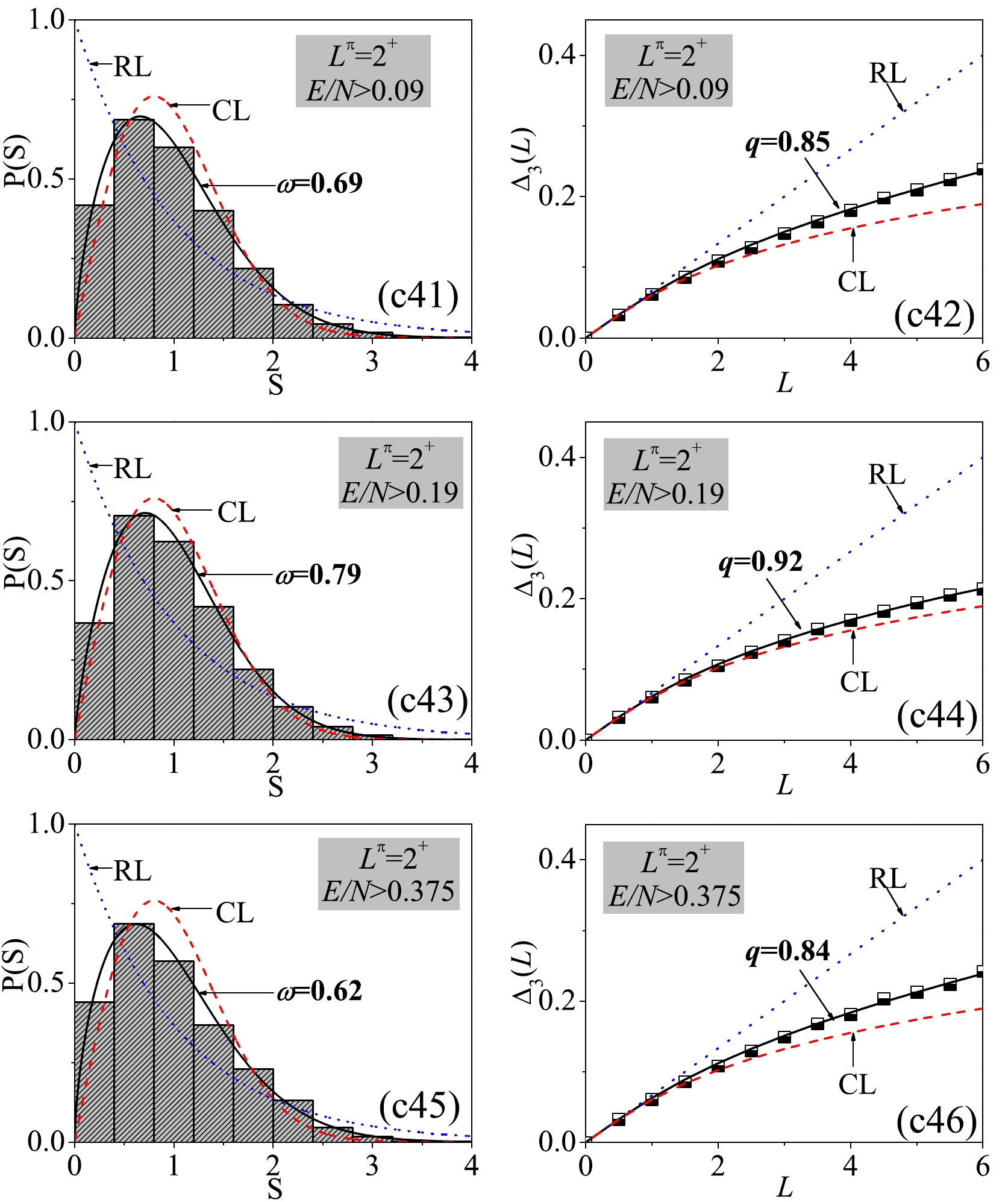
Figure 8. (color online) Same as in Fig. 7 but taking those bound above different energy cutoffs.
$ \begin{equation} \chi = \frac{2\sqrt{2}-(2\sqrt{2}+\sqrt{7})\eta}{2\eta}\, , \end{equation} $

(6) by connecting the approximate SU(3) symmetry with the AW arc of regularity [22]. We can observe that Eq. (6) describes the parameter trajectory being very close to the one described by (5) for
$ \eta\in[0.5,\; 1.0] $ .As schematically illustrated in Fig. 1, the trajectory of the AW arc may pass through two chaotic regions in the IBM phase diagram described by the parameters
$ (\eta,\; \chi) $ [10], whereas the two chaotic regions may cover most of the deformed area of the phase diagram. To analyze the spectral fluctuations in different scenarios, we select six parameter points to perform statistical calculations. These parameter points correspond to$(\eta,\; \chi) = (0.38,\; -{\sqrt{7}}/{2})$ ,$(0.47,\; -{\sqrt{7}}/{2})$ ,$(0.75,\; -{\sqrt{7}}/{2})$ ,$ (0.88,\; -1.032) $ ,$(0.88, -0.7)$ , and$ (1.0,\; -0.9) $ , which have been denoted by A, B, C, D, E, and F, respectively, as shown in Fig. 1. The points A, B, and C are used to illustrate three typical scenarios in the U(5)-SU(3) GSQPT, namely the spherical phase, critical point, and deformed phase; points D and E are selected to indicate the scenarios inside the triangle but lying on and off the AW arc; point F represents a typical case on the SU(3)-O(6) line, which in the large-N limit corresponds to a crossover [1].We can prove that the extreme values of the potential function (3) appear at either
$ \gamma = 0^\circ $ or$ \gamma = 60^\circ $ , whereas the latter can be equivalently realized by obtaining a negative β value owing to$ V(\beta,\gamma = 60^\circ) = V(-\beta,\gamma = 0^\circ) $ . The stationary points discussed here are defined as the extreme value points of the potential function$V(\beta)\equiv V(\beta,\gamma = 0^\circ)$ , namely those with$ \dfrac{\partial V(\beta)}{\partial\beta} = 0 $ . As an example, the potential curve at a typical parameter point inside the triangle is shown in Fig. 2 to illustrate the stationary point structure. Generally, the stationary points of a potential curve include the global minimum, global maximum, local minimum, local maximum, and$ |\beta|\rightarrow\infty $ limit point, which are denoted as$ V_{\mathrm{gmin}} $ ,$ V_{\mathrm{gmax}} $ ,$ V_{\mathrm{lmin}} $ ,$ V_{\mathrm{lmax}} $ , and$ V_{\mathrm{lim}} $ , respectively, as shown in Fig. 2. Among them,$ V_{\mathrm{lmin}} $ may correspond to a saddle point of$ V(\beta,\gamma) $ if we observe it from the degree of freedom of β and γ. At the mean-field level,$ V_{\mathrm{gmin}} $ and$ V_{\mathrm{gmax}} $ correspond only to the ground-state and highest excited energies, respectively. Therefore, more emphasis should be placed on$ V_{\mathrm{lmin}} $ ,$ V_{\mathrm{lmin}} $ , and$ V_{\mathrm{lmin}} $ . In terms of excitation energy, the related “critical” energies are further expressed as
Figure 2. (color online) Potential curve
$V(\beta)$ (in any unit) solved using (3) with$(\eta,\; \chi) = (0.9,-1.3)$ . The stationary points on the curve are signified by the dashed lines.$ E_{\mathrm{lmin}} = V_{\mathrm{lmin}}-V_{\mathrm{gmin}}, $

(7) $E_{\mathrm{lmax}} = V_{\mathrm{lmax}}-V_{\mathrm{gmin}}, $

(8) $E_{\mathrm{lim}} = V_{\mathrm{lim}}-V_{\mathrm{gmin}}\, . $

(9) We easily know that the energy scale in the “critical” energies is as same as the excitation energy per boson
$ E/N $ (in any unit), which means that the “critical” energies defined above can be directly used to compare the excitation energy$ E/N $ solved from the same Hamiltonian. -
To measure the spectral fluctuations in the IBM, we adopt two statistical measures here: the nearest neighbor level spacing distribution
$ P(S) $ [12] and the$ \Delta_3 $ statistics of Dyson and Mehta [13]. The spectral statistics should be performed to the so-called unfolded spectrum to be consistent with the requirements of the GOE [8]. First, we construct the staircase function of the spectrum,$ N(E) $ , defined as the number of levels below E with the level energies E solved from the Hamiltonian (1).$ N(E) $ is further separated into average and fluctuating parts$ \begin{equation} N(E) = N_{\mathrm{av}}(E)+N_{\mathrm{fluct}}(E)\, .\ \end{equation} $

(10) The average part can be expanded as a polynomial of sixth order in E [8, 14]:
$ \begin{equation} N_{\mathrm{av}}(E) = a_0+a_1E+a_2E^2+a_3E^3+a_4E^4+a_5E^5+a_6E^6\, \end{equation} $

(11) with the expanding parameters
$ a_i $ determined from the best fit to$ N(E) $ . Subsequently, the unfolded spectrum is obtained via the mapping$ \tilde{E_i} = N_{\mathrm{av}}(E_i) $ . With the unfolded spectrum, the nearest neighbor level spacings are obtained from$ \begin{equation} S_i = \tilde{E}_{i+1}- \tilde{E}_i\, , \end{equation} $

(12) and the distribution
$ P(S) $ is then given as the probability of two neighboring levels to be separated by a distance S. Specifically,$ P(S) $ will be shown as the histogram of the normalized spacing, and the results are further fitted to the Brody distribution [12]$ \begin{equation} P_\omega(S) = \alpha(1 + \omega)S^\omega \mathrm{exp}(-\alpha S^{1+\omega})\, \end{equation} $

(13) with
$ \alpha = \Gamma[(2 + \omega)/(1 + \omega)]^{1+\omega} $ . The Brody distribution interpolates between Poisson statistics$ (\omega = 0) $ characterizing a fully regular system and the Wigner distribution$ (\omega = 1) $ indicating a completely chaotic system [8]. As a result, the intermediate value with$ \omega\in[0,\; 1] $ provides a quantitative estimation of the quantum chaos in the spectrum.Spectral rigidity,
$ \Delta_3(L) $ , is a measure of the deviation of the staircase function from a straight line [13]. It is defined by$ \begin{equation} \Delta_3 (a,L) = \frac{1}{L} \mathrm{min}_{A,B}\int_a^{a+L} [N(\tilde{E})-A\tilde{E}- B]^2 {\rm d}\tilde{E}\, , \end{equation} $

(14) where A and B give the best local fit to
$ N(\tilde{E}) $ in the interval$ a\leq\tilde{E}\leq a+L $ , where L is the energy length of the interval. A rigid spectrum should provide a smaller$ \Delta_3 $ , whereas a soft spectrum provides a larger$ \Delta_3 $ . A smoother$ \Delta_3(L) $ can be obtained by averaging$ \Delta_3(a,L) $ over$ n_a $ intervals$ (a,\; a + L) $ :$ \begin{equation} \Delta_3(L) = \frac{1}{n_a}\sum_a\Delta_3(a,L)\, . \end{equation} $

(15) The successive intervals are set to overlap by
$ L/2 $ . In the concrete calculations, a useful formula [8]$ \begin{aligned}[b] \Delta_3(a,L) = &\frac{n^2}{16}-\frac{1}{L^2}\Bigg(\sum_{i = 1}^n\tilde{\epsilon}_i\Bigg)^2+\frac{3n}{2L^2}\Bigg(\sum_{i = 1}^n\tilde{\epsilon}_i^2\Bigg)\\ &-\frac{3}{L^4}\Bigg(\sum_{i = 1}^n\tilde{\epsilon}_i^2\Bigg)+\frac{1}{L}\Bigg(\sum_{i = 1}^n(n-2i+1)\tilde{\epsilon}_i\Bigg)\, \end{aligned} $

(16) with
$ \tilde{\epsilon}_i = \tilde{E}_i-(a+L/2) $ is often adopted. For the Poisson statistics, it is given by$ \begin{equation} \Delta_3^\mathrm{P}(L) = \frac{L}{15}\, , \end{equation} $

(17) whereas for the GOE (chaotic) case, it is approximately given by
$ \begin{equation} \Delta_3^{\mathrm{GOE}}(L) = \frac{1}{\pi^2}(\mathrm{log}L-0.0687)\, \end{equation} $

(18) for
$ L\gg1 $ . The exact form of$ \Delta_3 $ statistics for the GOE and Poisson limit can be solved using the integral [8]$ \begin{equation} \Delta_3(L) = \frac{2}{L^4}\int_0^L(L^3-2L^2r+r^3)\Sigma^2(r){\rm d}r\, \end{equation} $

(19) with
$ \Sigma^2(L) = L $ given for the Poisson statistics and$ \begin{aligned}[b] \Sigma^2(L) = &\frac{2}{\pi^2}\Big[\mathrm{ln}(2\pi L)+\bar{\gamma}+1+\frac{1}{2}\Big(\mathrm{Si}(\pi L)\Big)^2\\ &-\frac{\pi}{2}\mathrm{Si}(\pi L)-\mathrm{cos}(2\pi L)-\mathrm{Ci}(2\pi L)\\ &+\pi^2L\Big(1-\frac{2}{\pi}\mathrm{Si}(2\pi L)\Big)\Big]\, \end{aligned} $

(20) given for the GOE [8, 35]. In Eq. (20),
$ \bar{\gamma} $ is the Euler constant and Si (Ci) is the sine (cosine) integral. Similar to the Brody distribution, we can fit the calculated$ \Delta_3(L) $ with the parameterization [8, 12, 14, 36]$ \begin{equation} \Delta_3^{q}(L) = \Delta_3^{\mathrm{Poisson}}[(1-q)L]+\Delta_3^{\mathrm{GOE}}(qL),\; \; \; \; q\in[0,\; 1]\, \end{equation} $

(21) to obtain a quantitative estimation of the possible deviation of
$ \Delta_3(L) $ from the regular ($ q = 0 $ ) or chaotic limit ($ q = 1 $ ).To exemplify the
$ P(S) $ and$ \Delta_3 $ statistics, the calculated results for the spectra with$ L^\pi = 0^+,\; 2^+,\; 3^+ $ in the SU(3) limit are shown in Fig. 3. Since the SU(3) limit in the IBM corresponds to a completely integrable scenario, its dynamics are expected to be close to the regular limit (the Poisson statistics). As shown in Fig. 3, the results agree with such an expectation, resulting in$ \omega\sim0.12 $ ($ q\sim0.40 $ ) for the$ 0^+ $ spectrum and$ \omega\sim0.16 $ ($ q\sim0.43 $ ) for the$ 3^+ $ spectrum, which thus provides an example of regular system for reference. For the$ 2^+ $ spectrum in the SU(3) limit, we observe that the$ P(S) $ statistics indicate a negative value of ω, and the$ \Delta_3 $ statistics present values even larger than the Poisson statistics (the regular limit). This is a result of degeneracies and is related to missing labels according to the analysis given in [8]. In the SU(3) limit, the missing label is the quantum number K, which often provides two possible values$ K = 0,\; 2 $ for the$ 2^+ $ states in a given SU(3) irrep$ (\lambda,\; \mu) $ , but this may not affect the statistics for the$ 0^+ $ and$ 3^+ $ spectra as only one value is possible ($ K = 0 $ or$ K = 2 $ , respectively) for$ L^\pi = 0^+ $ and$ L^\pi = 3^+ $ [8]. Similar scenarios can also occur in the other symmetry limits or even in the cases that are close to a dynamical symmetry [6, 8], where the degeneracies accordingly become the approximate ones. Since the q values fitted from Eq. (21) cannot be negative, they are set as$ q = 0 $ in the following discussions if the$ \Delta_3 $ statistics is larger than the Poisson limit, similar to those shown in Fig. 3(f). Comparatively, ω appears to be always a reliable indicator of the spectral fluctuations in different cases.
Figure 3. (color online) (a)
$P(S)$ statistics for the states with$L^\pi = 0^+$ in the SU(3) limit with ω fitted from Eq. (13) are shown to compare the regular limit (RL) and chaotic limit (CL), which are denoted by the dotted and dashed lines, respectively; (b) Same as in (a) but for the$\Delta_3(L)$ statistics with q fitted from Eq. (21). Panels (c)-(f) show the same statistics as in (a) or in (b) but for$L^\pi = 3+$ and$L^\pi = 2^+$ . The calculation is performed for$N = 200$ . -
In this section, we discuss the spectral fluctuations at the selected parameter points and analyze their evolutional characters with the excitation energy. Note that the energy-dependent quantum statistics for the large-N
$ 0^+ $ spectra in the vicinity of the AW arc was previously performed in [14] with the states being divided into an equal number from a low to high energy. Here, we focus on more general scenarios, and the states are separated according to the energy cutoff instead of an equal number to perform the statistical calculations. In particular, both zero and nonzero spins are considered in the study.As shown above, the spectral fluctuations can be measured from the fitted ω and q values with
$ \omega\in[0,\; 1] $ and$ q\in[0,\; 1] $ . In the following, both ω and q are given as a function of the excitation energy with each value representing the result being solved from the$ P(S) $ or$ \Delta_3(L) $ calculations for all the states below a given energy cutoff$ E/N $ . Clearly, the higher the excitation energy, the more the states involved in the statistics. This means that any changes in the statistical results with the energy cutoff reflect only the evolution of the spectral chaos with the excitation energy. To obtain a reasonable statistical result, we require that the level numbers in the calculations at the lowest energy cutoff to be larger than 200. To complete the statistical analysis, we also perform the$ P(S) $ and$ \Delta_3(L) $ statistics from a high to low energy with each value of ω or q being solved from the statistics for all the states above a given energy cutoff. Similarly, the level numbers in the calculations at the highest energy cutoff are also required to be larger than 200. In summary, the energy dependence of the spectral fluctuations are tested from two directions, from low to high energy and from high to low energy. In the calculations, the total boson number is set as$ N = 200 $ , which means that we have a total of 3434$ 0^+ $ states, 6767$ 2^+ $ states, and 3333$ 3^+ $ states involved in the statistics calculations for each parameter point. For a higher angular momentum, the number of states for$ N = 200 $ may increase rather rapidly, which makes the production of the states significantly more difficult. Owing to computing time constraints, the present discussions are confined to$L^\pi = 0^+,\; 2^+,\; 3^+$ . In the following, the selected parameter points are divided into three groups: the points A, B, and C describe the U(5)-SU(3) transition, C and D characterize the scenario inside the triangle but lying on and off the AW arc, respectively, and point D represents a typical case in the SU(3)-O(6) transition. -
The U(5)-SU(3) transition at
$ \eta_c\simeq0.47 $ is proven to be a first-order GSQPT. The results solved from the parameter points A, B, and C in this transition are shown in Fig. 4–6, respectively. As shown in Fig. 4, the potential curve at the point A is rather simple with only one stationary point$ V_{\mathrm{lim}} $ lying between the global minimum and maximum. We further show that the entire spectrum for a given spin can be rather regular if we take all the levels into the statistical calculation, which yields, for example,$ \omega\approx0.15 $ and$ q\approx0.38 $ for$ L^\pi = 0^+ $ . However, the results suggest that the spectral fluctuations are not uniform in energy but the fitted ω and q values as functions of the excitation energy are shown to be consistent with each other during the entire evolutional process. Specifically, ω and q for a given$ L^\pi $ may gradually decrease as functions of the energy, as shown in panels (a1), (a3), and (a5). If observing the statistics from a high to low energy, we observe from panels (a2), (a4) and (a6) that the ω and q values present the nearly constant evolutions except for some small fluctuations appearing near$ E_{\mathrm{lim}} $ . The evolution of the spectral fluctuations in the spherical case with the simple potential configuration appears to be relatively simple.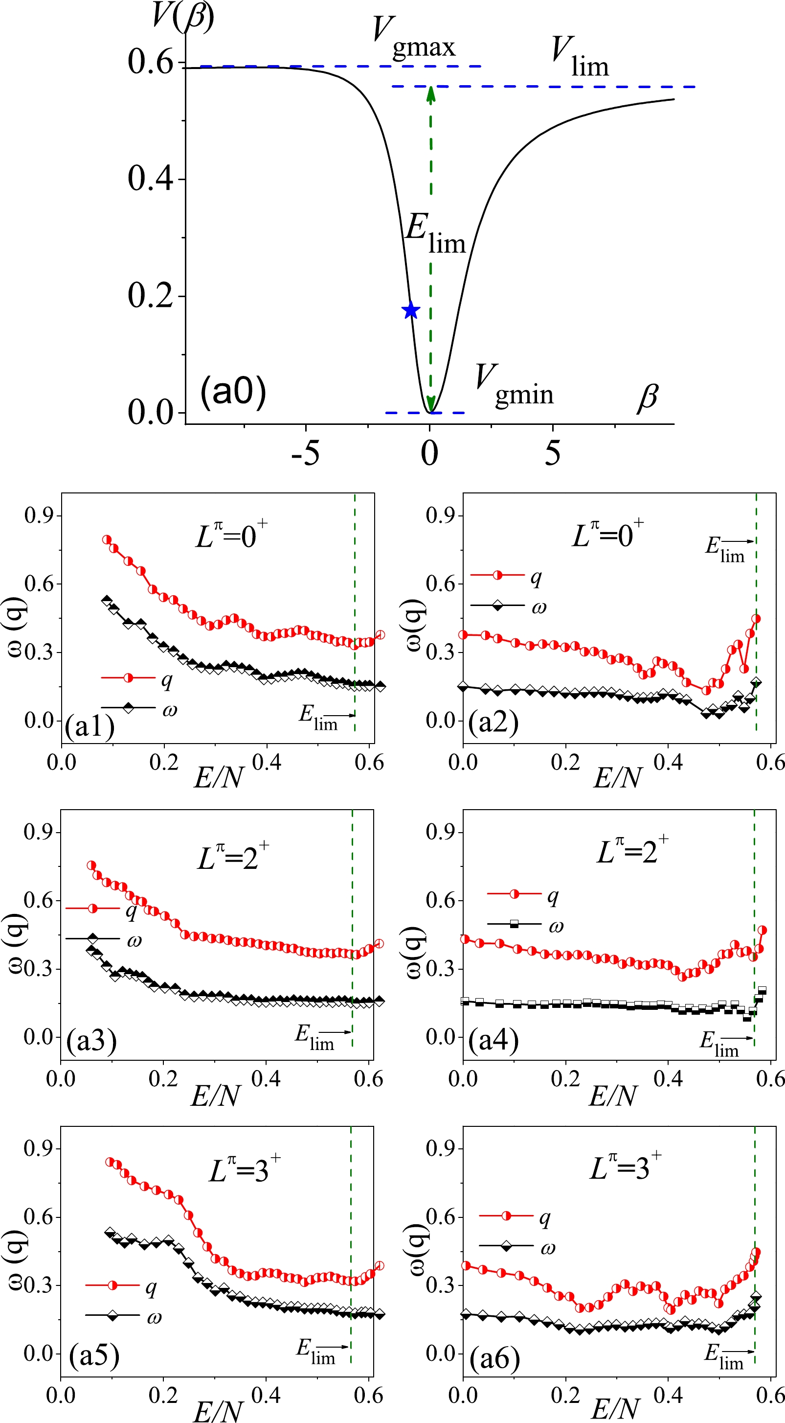
Figure 4. (color online) Parameter point A: (a0) Potential curve
$V(\beta)$ , with the blue star signifying$\frac{\partial^2V(\beta)}{\partial\beta^2} = 0$ ; (a1) Fitted ω and q values evolve as functions of the per-boson energy cutoff$E/N$ (any unit), with each$w(q)$ value being obtained from the$P(S)$ ($\Delta_3(L)$ ) statistics on all the$0^+$ levels below given$E/N$ ; (a2) Same as in (a1) but with the statistics on the levels above given$E/N$ . Panels (a3) and (a5) show the same results as in (a1) but for$L^\pi = 2^+$ and$L^\pi = 3^+$ , while (a4) and (a6) provide the same results as in (a2) but for$L^\pi = 2^+$ and$L^\pi = 3^+$ .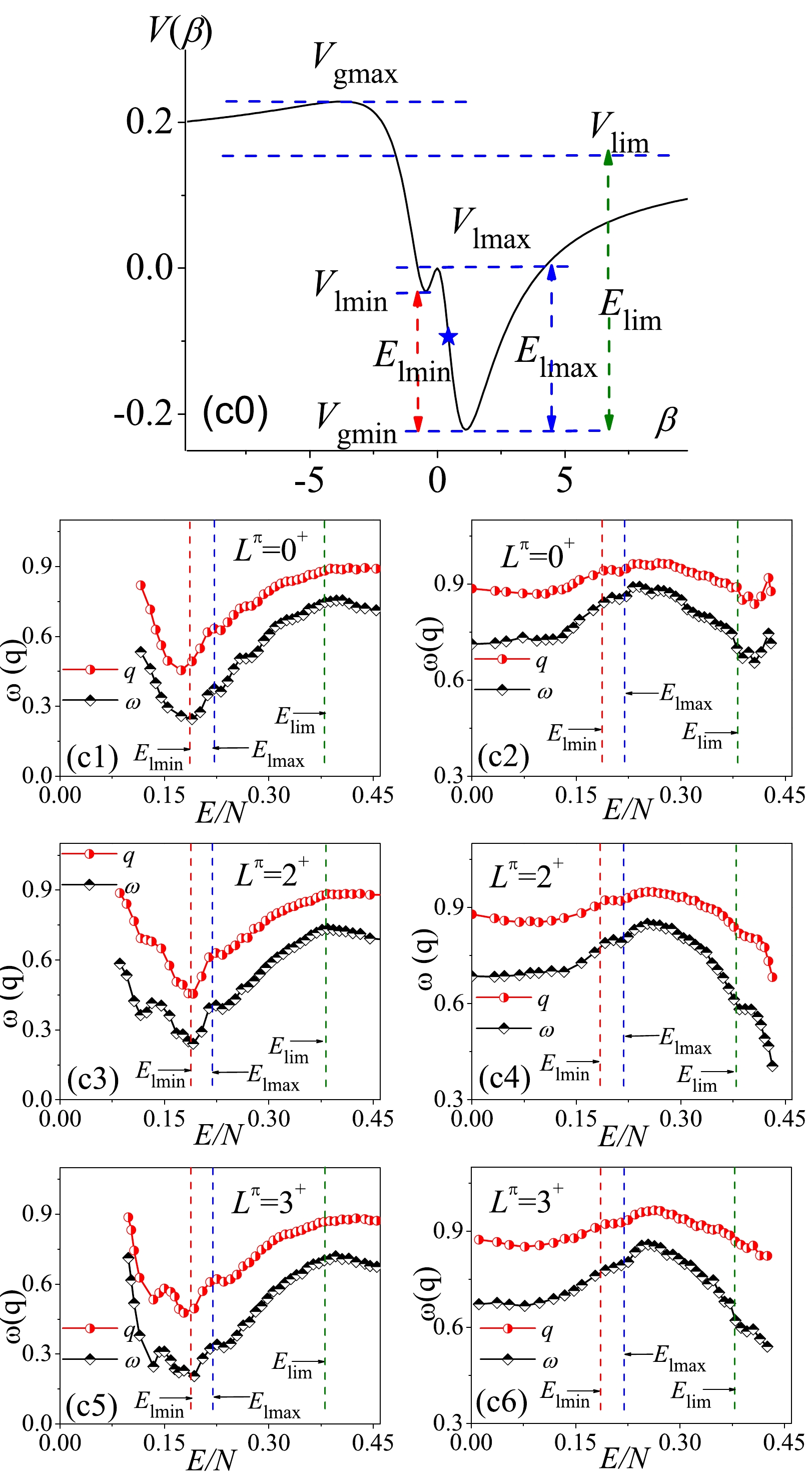
Figure 6. (color online) Same as in Fig. 4 but corresponding to the parameter point C.
A similar picture is observed at the critical point (the point B), as shown in Fig. 5. We observe that the global configuration of the potential curve at this point is as simple as the one at point A except that two degenerate minima appear on the bottom of the potential indicating the first-order GSQPT. As expected, the statistical results indicate that the entire spectrum at the critical point becomes less regular compared with the spherical case. For example,
$ \omega\approx0.45 $ is obtained in the former but$ \omega\approx0.15 $ is obtained in the latter if all the levels in the$ P(S) $ statistics are involved. Similar to the spherical case, the spectral fluctuations at the critical point are not uniform in energy. We can observe from (b1), (b3), and (b5) that ω and q exhibit the consistent evolutions with the excitation energy and may reach their maximal values at approximately$ E/N\sim0.2 $ , yielding$ \omega_{\mathrm{max}}>0.84 $ and$ q_{\mathrm{max}}>0.9 $ , respectively. However, this feature is not easy to illustrate from the mean-field structure as no stationary point appear nearby except the fastest changing point in$ V(\beta) $ observed at approximately$ E/N\sim0.15 $ , as shown in panel (b0). In addition, the consistency between the ω and q evolutions appears to be broken near$ E_{\mathrm{lim}} $ , as shown in panels (b2) and (b6). This can be crudely explained as follows: the calculated$ \Delta_3(L) $ results in the related cases arealready larger than the Poisson limit and thus are set with$ q = 0 $ . Such scenarios frequently occur only at$ \omega\sim0 $ .
Figure 5. (color online) Same as in Fig. 4 but corresponding to parameter point B. The inset in (b0) shows an amplified picture of the potential bottom with two degenerated minimal points indicating the first-order GSQPT at this parameter point.
The more interesting case should be the one at parameter point C because the potential
$ V(\beta) $ in a deformed system can hold a richer stationary point structure. As shown in Fig. 6(c0), three stationary points$ V_\mathrm{lmax} $ ,$ V_\mathrm{lmin} $ , and$ V_\mathrm{lim} $ are located in between$ V_\mathrm{gmax} $ and$ V_\mathrm{gmin} $ . More importantly, the effects of these stationary points can be clearly observed in the evolutions of the statistical results as a function of the excitation energy. As shown in Fig. 6(c1), the$ \omega(q) $ values for$ L^\pi = 0^+ $ present the non-monotonic evolutions with the minimal values appearing exactly at$ E_\mathrm{lmin} $ , above which the influence of the stationary point can be also clearly observed near$ E_\mathrm{lmax} $ . In addition to the similar evolutional features appearing around the stationary points, the$ \omega(q) $ values for$ L^\pi = 2^+,\; 3^+ $ exhibit small fluctuations near$ E/N\sim0.15 $ , as shown in panels (c3) and (c5). To some extent, this observation reflects the effects of nonzero spins on the spectral chaos. As further observed in panels (c2), (c4), and (c6), the influences of$ V_\mathrm{lmin} $ and$ V_\mathrm{lmax} $ on the spectral fluctuations have not been implicitly observed in the statistics from high to low energy but the influence of$ V_\mathrm{lim} $ can be still observed. This observation is not difficult to understand since the energy levels bound above$ V_\mathrm{lmax} $ in this case may occupy more than 75% of the total number for a given$ L^\pi $ . As a result, the influences of$ V_\mathrm{lmin} $ and$ V_\mathrm{lmax} $ on the spectral fluctuations may more or less be screened by the high-energy levels farther from the two stationary points.In the analysis given in [29], the stationary points
$ V_\mathrm{lmax} $ and$ V_\mathrm{lmin} $ were taken as the phase boundaries to perform the statistical analysis of the excited state quantum phase transitions (ESQPTs). Clearly, the present results further justify the reasonability of this. In addition, the analysis of the quantum optical models given in [37] indicate that the precursors of ESQPT phenomenon in a nonintegrable case may be accompanied by an abrupt emergence of spectral chaos. A similar scenario is suggested to occur here. Specifically, the results in Fig. 6(c1) indicate that the degree of chaoticity characterized by both ω and q will rapidly increase after$ E_\mathrm{lmin} $ , which is alternatively defined as the critical energy of the ESQPT in the U(5)-SU(3) transition [28]. Thus, we confirm that the ESQPT in the nonintegrable U(5)-SU(3) cases will be also accompanied by a sudden emergence of spectral chaos.To examine the energy dependence of the
$ P(S) $ and$ \Delta_3(L) $ statistics closely, we select the cases at three different energy cutoffs from the panels (c2) and (c4) of Fig. 6, respectively. We observe from Fig. 7 and Fig. 8 that the statistical results for$ L^\pi = 2^+ $ may differ significantly at different cutoffs. It is given by$ \omega = 0.25 $ ($ q = 0.45 $ ) for the spectrum below$ E/N = 0.19 $ but by$ \omega = 0.79 $ ($ q = 0.92 $ ) for that above$ E/N = 0.19 $ . Since$ E/N = 0.19 $ is very close to the critical energy$ E_\mathrm{lmin} $ , the results confirm again that the spectral fluctuations can be significantly different by taking the stationary point$ V_\mathrm{lmin} $ as a boundary, as performed in [29]. In summary, the spectral fluctuations in the deformed phase of the U(5)-SU(3) GSQPT are observed to be more energy dependent owing to the richer stationary point structure.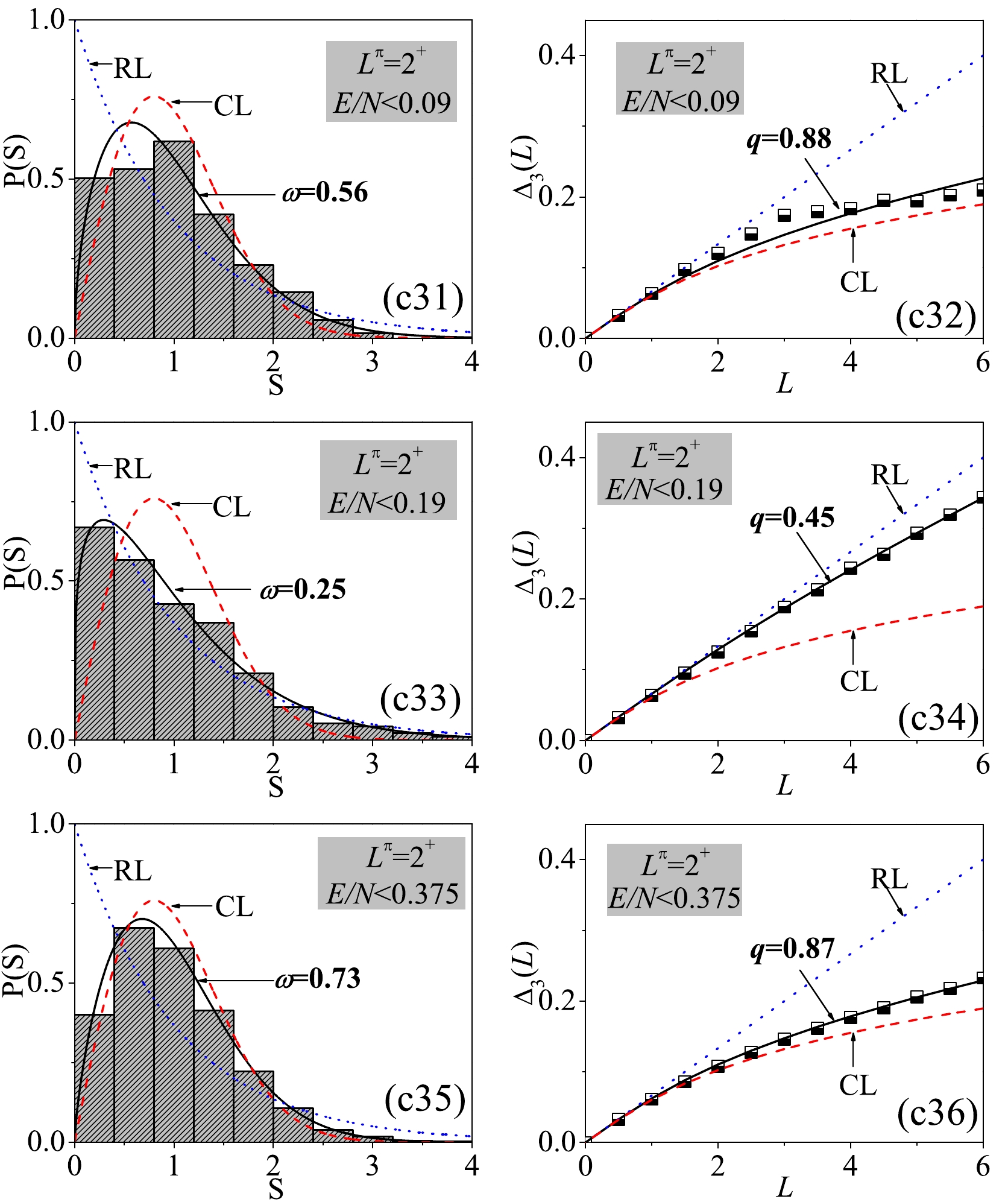
Figure 7. (color online) Statistics for the parameter point C shown with the statistical sample selected as the
$2^+$ levels bound below different energy cutoffs. -
In the triangle phase diagram, parameter points D and E describe the scenarios on and off the AW arc, respectively. The systems on the AW arc are always expected to produce regular spectra for zero [14] and nonzero spins [10]. As shown in Fig. 9, the results indicate that the entire spectrum on the AW arc is indeed very regular when involving all the levels in statistical calculations for a given
$ L^\pi $ . This is highlighted by the results for$ L^\pi = 2^+ $ , as observed in panels (d3) or (d4), where we observe that the statistical calculations for the entire$ 2^+ $ spectrum yield$ \omega\sim0 $ and$ q\sim0 $ . Nonetheless, the energy dependence of the spectral fluctuations on the AW arc can be still clearly observed [14]. In particular, we observe that the ω and q values as a function of the excitation energy may noticeably change near$ E_{\mathrm{lmax}} $ . The results in panel (d1) indicate that the spectral fluctuations in the$ 0^+ $ states will decrease until$ E_{\mathrm{lmax}} $ and then slightly increase, followed by another decrease near$ E_{\mathrm{lim}} $ . This means that the highest-lying states are always regular but the states near or below the stationary point$ V_{\mathrm{lmax}} $ are also relatively regular. This picture actually agrees with the classical analysis of the AW arc given in [19], where the results for the regular fraction$ f_{\mathrm{reg}} $ (see Fig. 4 in [19]) indicate that the relative regularity of the AW arc can, to some extent, be enhanced near the absolute energy$ E_{\mathrm{cl}} = 0 $ corresponding to the stationary point$ E_{\mathrm{lmax}} $ discussed here.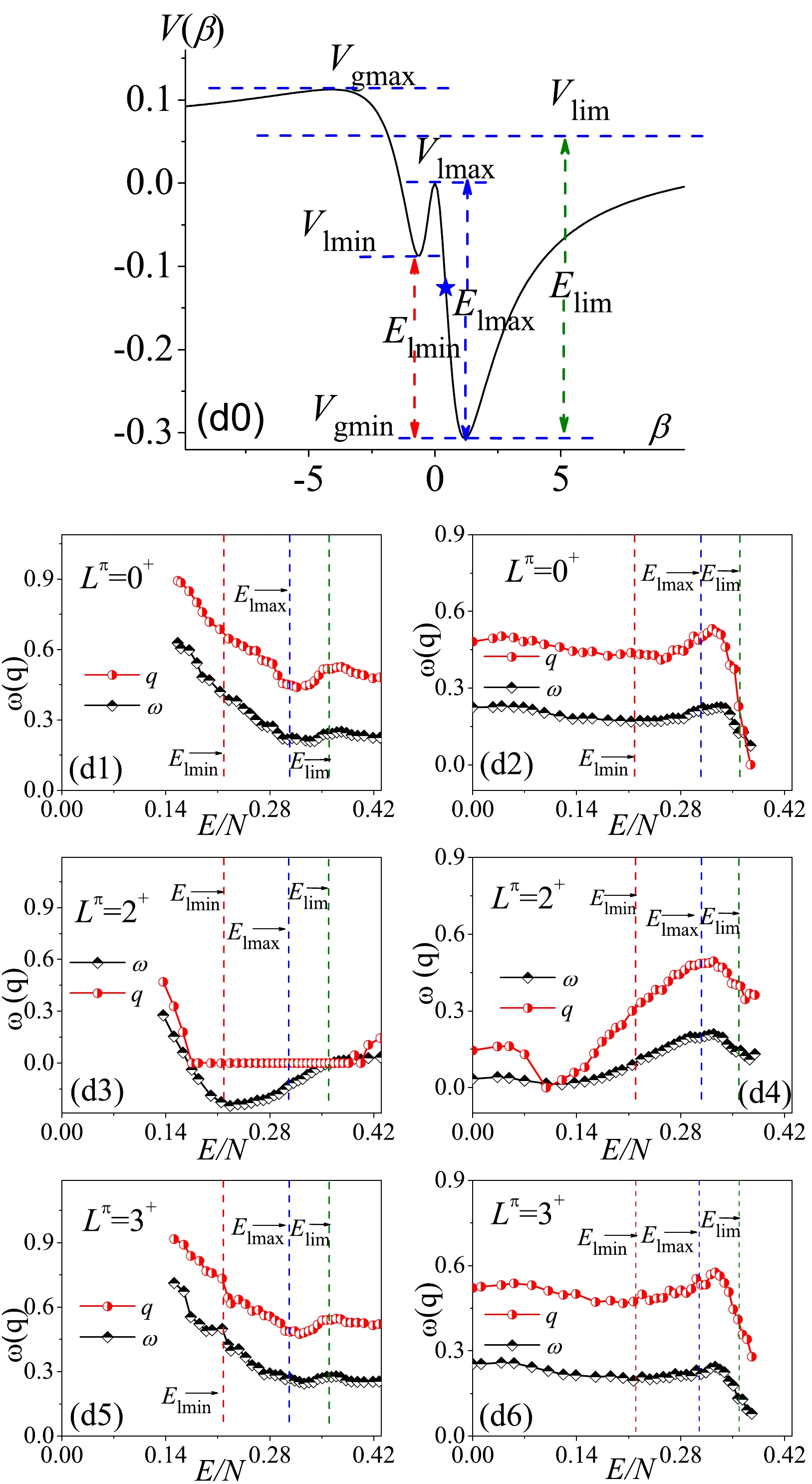
Figure 9. (color online) Same as in Fig. 4 but corresponding to parameter point D (on the AW arc).
In contrast, the ground state and the adjacent lowest states for the AW arc should be also regular according to the analysis given in [19]. However, this point cannot be directly reflected from the
$ P(S) $ and$ \Delta_3(L) $ calculations presented here since the statistics require a sufficient number of levels rather than a single ground state or a few number of lowest-lying states. As a result, the relatively larger$ \omega(q) $ values at low energy shown in the panel (d1) only imply that some relatively chaotic states may occupy a certain proportion below the corresponding energy cutoff. The results for the regular fraction given in [19] also indicate that the degree of regularity on the AW arc can be largely reduced in between the ground state and absolute energies$ E_{\mathrm{cl}} = 0 $ . However, such a "chaotic" character at low energy will be rapidly smoothed out when involving more higher energy states in the statistical calculations. For example, if the energy cutoff is taken as the saddle point energy$ E_{\mathrm{lmax}} $ , the degree of chaos for the$ 0^+ $ spectrum may decrease to$ \omega\sim0.3 $ , as shown in panel (d1).We can observe from panels (d5) and (d6) that the energy dependence of the spectral fluctuation for
$ L^\pi = 3^+ $ are very similar to the one for$ L^\pi = 0^+ $ . In contrast, the spectral fluctuations for$ L^\pi = 2^+ $ exhibit some special features. An impressive aspect is that ω will become negative in the energy interval$ [E_\mathrm{lmin},\; E_\mathrm{lim}] $ with$ q = 0 $ , as shown in panel (d3). When performing the statistical calculations from high to low energy, the$ q = 0 $ results may also appear at very low energy$ E/N\sim0.1 $ , as shown in panel (d4). According to convention, the q values will be set by zero when the$ \Delta_3(L) $ results are larger than the Poisson limit. Similar to the case in the SU(3) symmetry discussed in Sec. II.B, the results$ \omega<0 $ and$ q = 0 $ shown here may also be a result of degeneracies. We then deduce that the degeneracies (approximate) in the$ 2^+ $ spectrum may be associated with the SU(3) quasidynamical symmetry [21, 22] since its parameter trajectory characterized by$ E(2_\beta^+) = E(2_\gamma^+) $ was observed to be very close to the AW arc, therefore suggesting a symmetry-based interpretation of the AW arc. The present results indicate that such a symmetry-based explanation of the AW arc can be tested from the point of statistics on the$ 2^+ $ states. However, indicating which$ 2^+ $ states are approximately degenerate by directly observing their level energies in a symmetry-broken case is difficult. In addition, the validity of the underlying SU(3) quasidynamical symmetry inside was suggested to be limited to low-lying states in the large-N limit [21]. Therefore, whether the negative ω values and$ q = 0 $ can be fully explored by the approximate degeneracies requires further studying, which may be discussed elsewhere.For the scenario off the AW arc, we observe from Fig. 10 that the potential curve at the point E is very similar to the one at the point D. Both of them have three stationary points lying in between
$ V_\mathrm{gmax} $ and$ V_\mathrm{gmin} $ . However, the spectral fluctuations in the two scenarios are very different and even evolve in the opposite directions. First, the spectra at the point E are observed to be significantly more chaotic than those on the arc. For example, the$ P(S) $ statistics on all the states with$ L^\pi = 2^+ $ yield$ \omega\sim0 $ and$ q\sim0 $ for point D but$ \omega>0.6 $ and$ q>0.8 $ for point E. In addition, the results given in panels (e1), (e3), and (e5) indicate that spectral fluctuations at point E may increase with the excitation energy until$ E_{\mathrm{lmax}} $ and then turn to a slow decrease. A notable observation is that the$ \omega(q) $ values for$ L^\pi = 2^+ $ exhibit a sudden enhancement at approximately$ E_\mathrm{lmin} $ , as shown in panel (e3). All these features reflect only the effects of the stationary points on the spectral fluctuations at point E. In contrast, the relatively smoother evolutions can be observed when performing the statistical calculations from high to low energy, as shown in panels (e2), (e4), and (e6).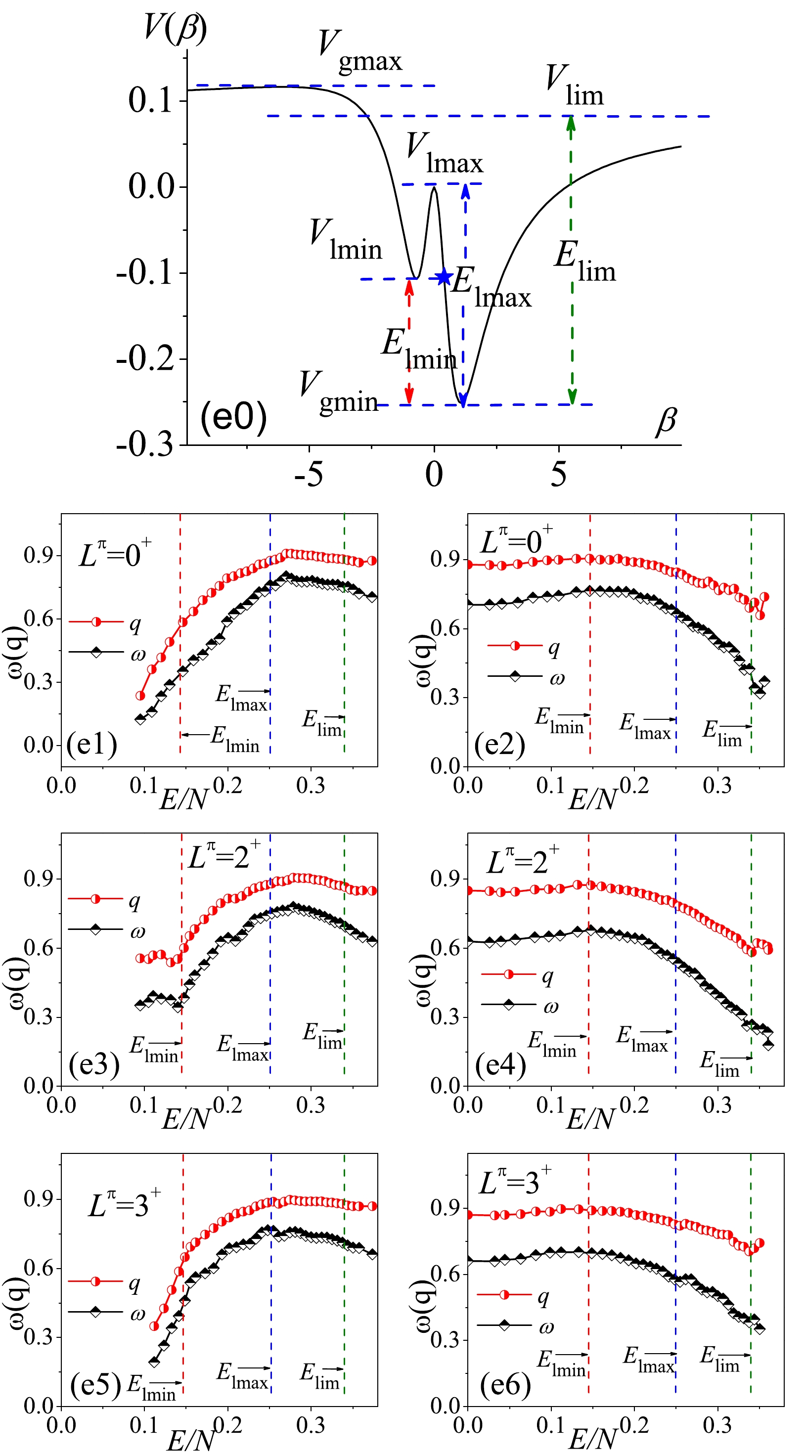
Figure 10. (color online) Same as in Fig. 4 but corresponding to the parameter point E.
To make a closer comparison between the cases on and off the AW arc, we extract the concrete statistics on the levels below
$ E_\mathrm{lmin} $ and$ E_\mathrm{lmax} $ in the two cases from Fig. 9 and Fig. 10. As shown in Fig. 11, the results indicate that spectral fluctuations for$ L^\pi = 0^+ $ below$ E_\mathrm{lmin} $ do not have a significant difference in between two cases with$ \Delta\omega = |\omega_1-\omega_2| = 0.07 $ and$ \Delta q = |q_1-q_2| = 0.11 $ , where$ \omega(q)_{1,2} $ represent the results in the two cases. However, the spectral fluctuations on the arc decreases dramatically if more states are involved in the statistics by taking the energy cutoff$ E_\mathrm{lmax} $ . Instead, the ones off the arc may become considerably chaotic with$ \omega = 0.76 $ and$ q = 0.88 $ . Accordingly, the differences in between two cases are the greatest for$ \Delta\omega = 0.52 $ and$ \Delta q = 0.42 $ , which are even larger than the results involving all the$ 0^+ $ levels into the statistics,$ \Delta\omega = 0.48 $ and$ \Delta q = 0.40 $ . This observation also agrees with the classical analysis of the AW arc in [19] that the relative regularity of the arc is most significant only at approximately the absolute energy$ E_{\mathrm{cl}} = 0 $ corresponding to$ E_\mathrm{lmax} $ . As shown in Fig. 12, the spectral fluctuations for$ L^\pi = 2^+ $ are very similar to those for$ L^\pi = 0^+ $ for the arc with relatively small$ \omega(q) $ at the low energy cutoff and large$ \omega(q) $ at the high energy cutoff. In contrast, the$ 2^+ $ spectrum on the AW arc is observed to be over regular even at the high energy cutoff with a negative ω value, which are consistent with those shown in Fig. 9(d3). As shown in Fig. 13, the results for$ L^\pi = 3^+ $ confirm that the regularity on the Arc are pronounced near$ E_\mathrm{lmax} $ , with the differences between the two case reaching$ \Delta\omega = 0.50 $ and$ \Delta q = 0.41 $ at this energy cutoff.
Figure 11. (color online) For a close comparison between points D (on the arc) and E (off the arc), the statistics for the
$0^+$ levels bound below$E_\mathrm{lmin}$ and$E_\mathrm{lmax}$ in the two cases are shown.
Figure 12. (color online) Same as in Fig. 11 but for the
$2^+$ spectra.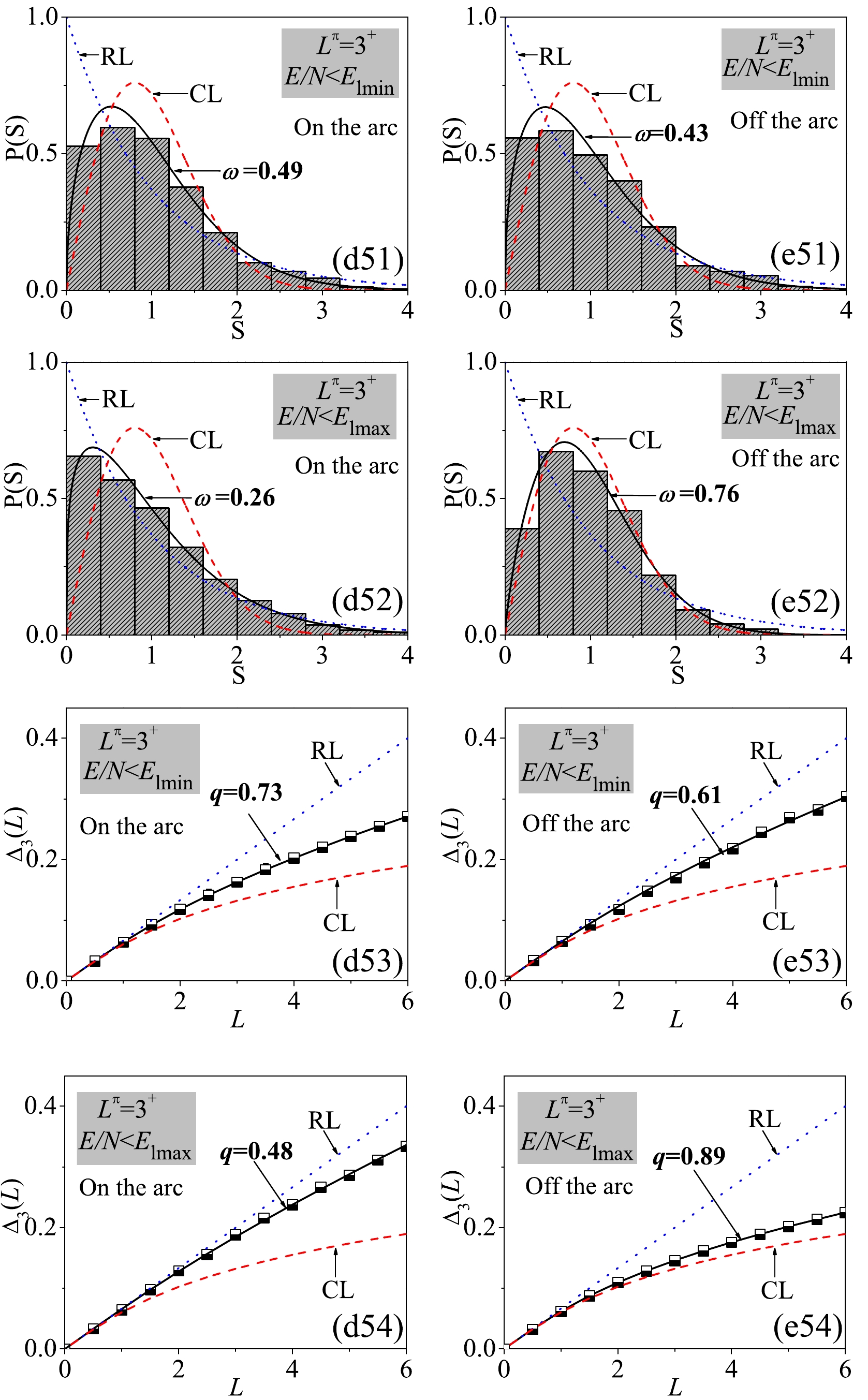
Figure 13. (color online) Same as in Fig. 11 but for the
$3^+$ spectra. -
The parameter point F represents a typical case in the SU(3)-O(6) transition. As shown in Fig. 14(f0), the potential curve at this point has only two stationary points lying in between
$ V_\mathrm{gmin} $ and$ V_\mathrm{gmax} $ as its local maximal point at$ \beta = 0 $ may coincide with its global maximum. The spectra for$ L^\pi = 0^+,\; 2^+,\; 3^+ $ are all shown to be relatively chaotic with$ \omega>0.6 $ and$ q>0.8 $ if all the levels are involved in the statistics for a given spin. As in the other cases, the spectral fluctuations in this case are not uniform in energy, and the energy-dependence can be partially illustrated based on its mean-field structure. For example, the$ \omega(q) $ values as functions of the excitation energy may reach their maxima near$ E_\mathrm{lim} $ as shown in panels (f2), (f4), and (f6). The influence of$ E_\mathrm{lmin} $ on spectral fluctuations can be also observed by observing panel (f3), in which the results imply that the spectral chaos will rapidly increase after this energy point. All these only indicate the effects of the stationary points on the spectral fluctuations in this case.
Figure 14. (color online) Same as in Fig. 4 but for those corresponding to the parameter point F.
-
The energy dependence of the spectral fluctuations in the IBM and its connections to the mean-field structures are investigated for the cases across the U(5)-SU(3) GSQPT, near the AW arc, and in the SU(3)-O(6) transition. Two statistical measures, the nearest neighbor level spacing distribution
$ P(S) $ and the$ \Delta_3 $ statistics of Dyson and Mehta, are applied to inspect the spectral fluctuations in each case. We observe that the spectral fluctuations as a function of the energy cutoff may exhibit different evolutional behaviors in different cases, but their behaviors are all shown to be closely related to the corresponding mean-field structures. Specifically, most of the sudden changes in the fluctuational evolutions can be attributed to the effects of the stationary points, particularly for the cases in the deformed area of the phase diagram, where the ESQPT phenomena can be observed around the same stationary points [28]. These findings confirm again the role of the mean-field structure in understanding excited state properties. Another new finding is the appearance of negative ω values indicating the approximate degeneracies in the$ 2^+ $ spectrum on the AW arc. This may provide a statistical signature of the approximate SU(3) symmetry along the AW arc [21, 22]; however, this requires to be further proved. The present large-N analysis not only add new information to the chaotic map of the IBM but also offer a reference for the study of spectral fluctuations in the Bohr-Mottelson model since the model may directly link the large-N limit of the IBM [1]. The discussions on spectral fluctuations can be extended to discuss the fluctuations in other quantities such as the$ B(E\lambda) $ transitions [14] or to other algebraic models including those for two-fluid systems [38–41], where the stationary point and phase structures may be much richer than the present case [38, 40]. In addition, classical measures [6] can be also applied to reveal the energy dependence of spectral fluctuations in the IBM. The related research is in progress.
Spectral fluctuations in the interacting boson model
- Received Date: 2022-04-18
- Available Online: 2022-10-15
Abstract: The energy dependence of the spectral fluctuations in the interacting boson model (IBM) and its connections to the mean-field structures are analyzed by adopting two statistical measures: the nearest neighbor level spacing distribution


 DownLoad: