


 Abstract
 HTML
HTML Reference
 Related
 PDF
PDF


-
The direct detection of dark matter particles, especially the weakly interacting massive particles (WIMPs), is being actively carried out by a couple of experiments worldwide [1]. In recent years, the PandaX-II experiment located in the China Jinping Underground Laboratory (CJPL) [1–3], which uses the technology of dual phase liquid xenon time projection chambers (TPCs), has pushed the limits of the cross section between WIMPs and nucleons to a new level for most of the possible WIMP masses; other experiments of the same type are also being performed [4–10]. The scattering of incident particles with xenon atoms in the TPC may produce a prompt scintillation
$ S1 $ , which results from the de-excitation of xenon atoms and the recombination process of some ionized electrons. Some electrons escaping from the recombination may drift along the electric field inside the TPC and be extracted into the gaseous region, producing the proportional electroluminescent scintillation$ S 2 $ [11, 12]. The detected$ S 1 $ and$ S 2 $ signals are used to reconstruct the scattering event in the data analysis. Due to the low probability of scattering events between WIMPs and ordinary matter, a good physical event requires only one pair of physically correlated$ S 1 $ and$ S 2 $ within the maximum electron drift time window inside the TPC. In the last results of the PandaX-I experiment [13], it was realized that the accidental coincidence of isolated$ S 1 $ and$ S 2 $ within the window comprises a new type of background, which promotes a number of events in the signal parameter space to search for WIMPs. Understanding this type of background and the development of methods to suppress it become important for the improvement of dark matter detection sensitivity. In the data analysis of PandaX-II with full exposure, we conducted a thorough study of the accidental background and presented an accurate estimation of its level for all three data taking runs (9, 10, and 11) [4].In this article, we present a detailed introduction on the study of accidental background in PandaX-II in Sec. I. In Sec. II, we provide a brief introduction to the PandaX-II TPC, signals, and backgrounds. Then, we discuss the possible origin of the accidental background in Sec. III, with the estimation of its level presented in Sec. IV. The application of the boost-decision-tree (BDT) method to suppress the background is given in Sec. V, with the performance presented. Finally, we give a brief summary and outlook in Sec. VI.
-
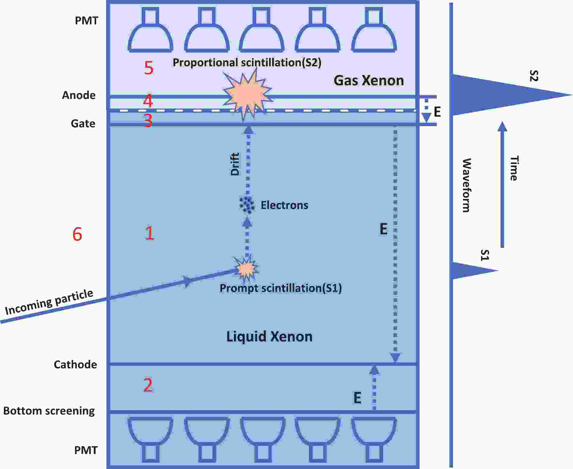
A detailed description of the PandaX-II TPC is presented in Ref. [7]. A more detailed schematic view of the TPC is presented in Fig. 1. The near-cylindrical shaped TPC confined by polytetrafluoroethylene (PTFE) walls, contains both gaseous xenon (top) and liquid xenon (bottom) in its volume. Scintillation light generated inside the TPC is detected by the two arrays of photo-multiplier tubes (PMTs) located on the top and bottom region, respectively. The cathode in the bottom part of the TPC and the gate electrode right below the liquid surface provide the drift electric field for ionized electrons and define the sensitive region of the detector (region 1 in Fig. 1).
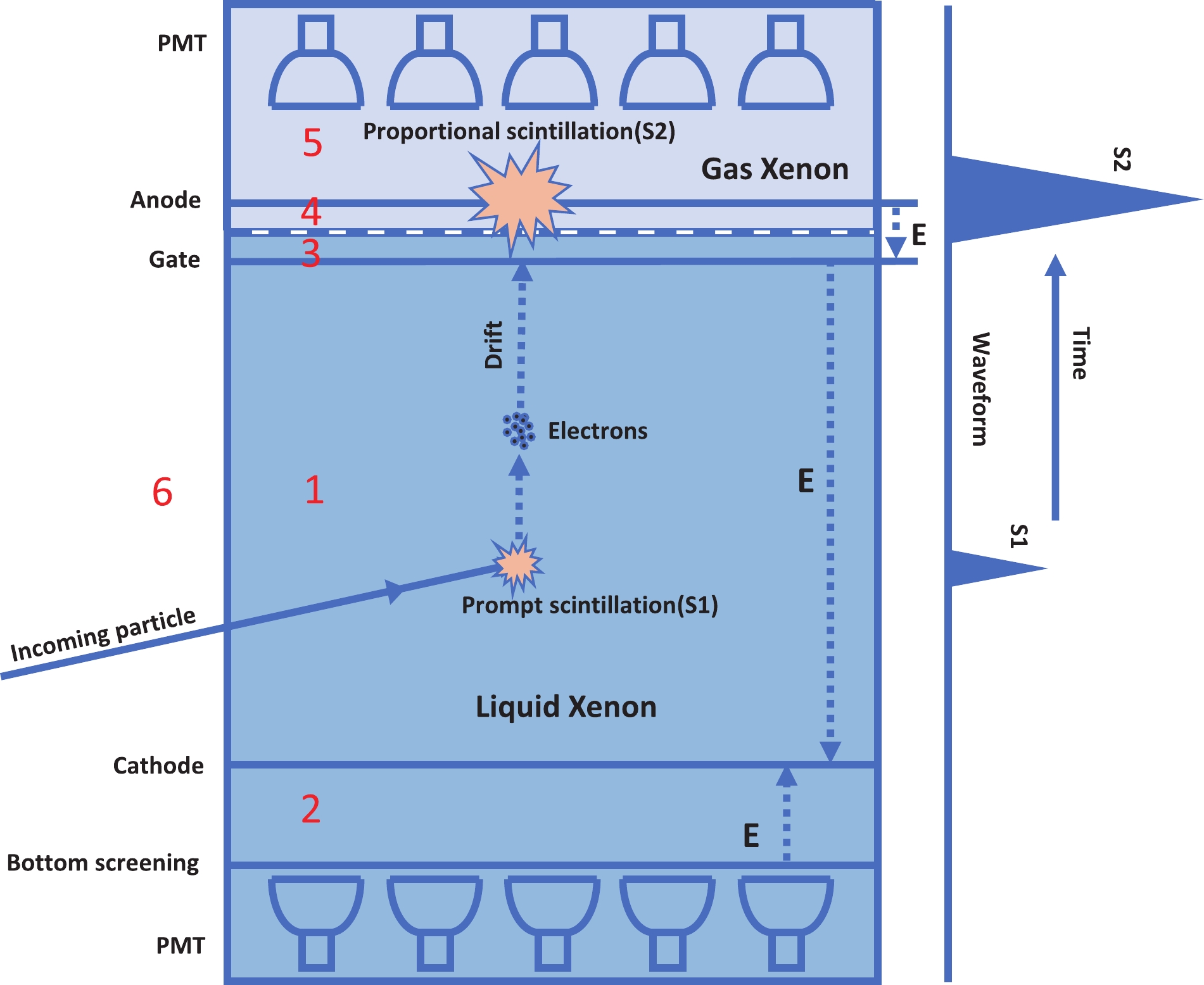
Figure 1. (color online) Schematic view of the TPC of PandaX-II, with six regions labeled with numbers: 1. the liquid part below the gate and above the cathode; 2. the liquid part below the cathode; 3. the liquid part above the gate; 4. the gas part below the anode; 5. the gas part above the anode; 6. the parts outside the inner PTFE walls. A recoil event in region 1 may produce
$ S 1 $ and$ S 2 $ signals at different regions in the detector with a time delay.Deposited energies by scattering events inside the sensitive region result in a
$ S1 $ signal, typically with a time spreading① smaller than 150 ns, which is a very short time, while the possible$ S 2 $ signal will be produced after a time delay, due to the limited drift velocity of ionized electrons inside liquid xenon. The drift velocity of the electrons depends only on the electric field strength; thus, the time difference between the physically correlated$ S 1 $ and$ S 2 $ can be used to calculate the vertical position of a scattering event. The maximum drift time for electrons in the sensitive region is$ 350\pm8 $ μs in Run 9 and$ 360\pm8 $ μs in Runs 10 and 11, due to the different drift fields [4]. When a "trigger" signal, observed during the ordinary recording of data, exceeds the pre-defined threshold, the digitized waveform of all the PMTs within a window of 500 μs before and after the trigger time is recorded as an event. The data processing steps calculate the baseline of each recorded waveform, search for a "hit" exceeding a given threshold of 0.25 photoelectrons (PE), and cluster the overlapped hits into signals. Events of single scattering (with only one$ S 1 $ and$ S 2 $ reconstructed) are selected, and then filtered by the quality cuts to search for the possible rare scattering from WIMPs.Recognition, understanding, and suppression of the different types of backgrounds are critical in the data analysis of WIMP searching experiments because the desired signal rate is very low. In the PandaX-II experiment, the backgrounds can be categorized into four types. The electron recoil (ER) background, mainly from the radioactive isotopes in the detector material or in the xenon target, has been studied and understood with the ER calibration data and Geant4-based Monte Carlo (MC) simulations [14, 15]. The nuclear recoil (NR) background, mainly from neutrons produced by the (α, n) process or spontaneous fission of isotopes in detectors, has been estimated by the correlated high energy gamma events with the help of simulation [16]. The surface background is created by daughters of 222Rn attached on the inner surface of the TPC and has a suppressed
$ S 2 $ due to the charge loss on the PTFE wall. The level of surface background is estimated with a data driven method [4, 17]. Finally, the nonphysical accidental background results from the false pairing of unrelated$ S 1 $ and$ S 2 $ signals. A large proportion of the accidental background events have relatively small$ S 2 $ signals and thus are not easily distinguished from the physical NR events (neutron or WIMPs) by investigating the ratio of$ S 2/S 1 $ only. Effective suppression of the accidental background will improve the discovery sensitivity of WIMPs greatly. -
In the TPC, some
$ S 1 $ or$ S 2 $ -like signals may be produced without any other signals from the same source observed by detector. We call these signals "isolated." Since the events with a pair of$ S 1 $ and$ S 2 $ are used to search for dark matter, the isolated signals appearing in the same drift window may be paired, resulting in the accidental background. -
The origins of isolated
$ S 1 $ s may be physical or non-physical. The physical origins might be in the following:● tiny sparks on the TPC electrode; thus, no electrons are produced;
● scattering events in the region between the cathode and the screening electrode of the bottom array (region 2 in Fig. 1), which prevent electrons from drifting into the gas xenon; thus, no
$ S 2 $ could be produced;● physical events occur near the bottom wall of the detector, resulting in a loss of all electrons owing to an imperfect drift field; thus, no
$ S 2 $ is produced;● scattering events above the anode in the gaseous region (region 5 in Fig. 1), which prevent electrons from entering the region below the anode; thus, no
$ S 2 $ is produced;● signals produced by single electron extract into the gas region, which are mis-identified as
$ S 1 $ s;● possible light leakage from scattering events outside the TPC (region 6 in Fig. 1).
The dominant non-physical origin of isolated
$ S 1 $ is from the dark noise of the PMT, which produce small hits in the readout waveform of each PMT. During the event reconstruction, a valid signal should contain overlapped hits from at least three PMTs. The relatively high rate of dark noise (average rates are 1.9, 0.17, and 0.23 kHz per PMT for Runs 9, 10, and 11, respectively) makes the formation of small$ S 1 $ -like signals via the random coincidence of the dark noises possible. Since these signals have a contribution from the top PMTs, their top-bottom asymmetry (discussed in Sec. V.A) should not be$ -1 $ . -
The
$ S 2 $ signals are from the electroluminescent of electrons in the gas region. The isolated$ S 2 $ signals, without exception, resulted from the same process. The origin of isolated$ S2 $ can be categorized into four types:● real scattering event in the sensitive region with small energy deposition; the weak
$ S 1 $ is not recognized due to the detection efficiency;● real scattering event in the sensitive region that it is too close to the liquid surface, resulting in overlapped
$ S 1 $ and$ S 2 $ signals, which are recognized as one$ S 2 $ ;● real scattering event in the region above the gate but below the anode (region 3 and 4 in Fig. 1), resulting in overlapped
$ S 1 $ and$ S 2 $ signals recognized as one$ S 2 $ ; the signal may have a smaller width and asymmetrical shape;● the electrons generated with large energy deposition may not be extracted into the gas region completely. The rest of the electrons gather on the liquid surface and are released into the gas randomly, producing electroluminescent directly.
-
Since the isolated signals are independent from each other, the level of accidental background can be calculated by the rates of isolated
$ S 1 $ and$ S 2 $ signals, assuming they follow a uniform distribution over time in a selected period with same run conditions. Estimation of the rates of these signals becomes important in this study.For each of the data taking runs, the average rates
$ \bar{r}_1 $ and$ \bar{r}_2 $ for isolated S1 and$ S 2 $ , respectively, are computed by the time weighted average of the corresponding rates:$ \bar{r}_1 = \frac{1}{\displaystyle\sum_i T_i}\sum_i r_{1i}\cdot T_i, $

(1) $ \bar{r}_2 = \frac{1}{\displaystyle\sum_i T_i}\sum_i r_{2i}\cdot T_i, $

(2) where
$ T_i $ ,$ r_{1i} $ , and$ r_{2i} $ are the duration, and rates of isolated$ S 1 $ and$ S 2 $ for each selected period i, respectively. The uncertainties of the rates are calculated as the unbiased standard errors of the mean value. -
To calculate the rate of isolated
$ S 1 $ , we need to recognize this type of signal correctly in the data. Three methods have been developed to search for the isolated$ S 1 $ within the range of$ (3,100) $ PE, which covers the energy region of searching for dark matter. One is based on a special type of "random trigger" data set, with the event triggered by hardware randomly. The other two methods are based on the dark matter search data. We describe these three methods here. -
This method is used to search isolated
$ S 1 $ events in the random trigger data. The events should satisfy all the required data quality cuts mentioned in Ref. [4]. The rate$ r_1 $ in one run can be calculated easily by②$ r_1 = \frac{n_{iS 1}}{T}, $

(3) where
$ n_{iS 1} $ is the number of qualified isolated$ S 1 $ , and T is the live time of the random trigger events. This method is unbiased, and is used to estimate the accidental background level in Run 10 [5]. Due to the short time of data taking with random trigger, the long term evolution of the rate can not be extracted. No random trigger data taking was performed in Run 9, so this method can only work in Runs 10 and 11. -
In this method, the isolated
$ S 1 $ is defined as small$ S 1 $ signals before the triggered$ S 1 $ , which has no paired$ S 2 $ within the window of maximum drift time (see Fig. 2). The triggered$ S 1 $ should be larger than 100 PE. The time difference$ \Delta t $ (see Fig. 3) between the isolated$ S 1 $ and the triggered$ S 1 $ is used directly in the simulation of accidental background by pairing the selected isolated$ S 1 $ and$ S 2 $ signals (see following section). Therefore, we require that$ \Delta t $ be within the window of$ (10,\;350) $ μs for Run 9 or$ (10,\;360) $ μs for Runs 10 and 11 before the triggered$ S 1 $ by considering the cut on the drifting time.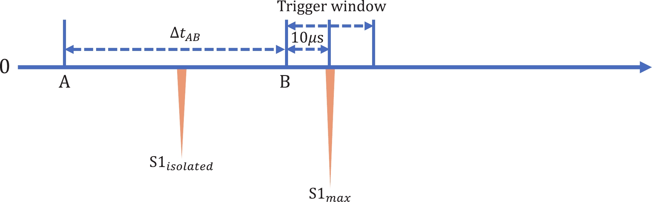
Figure 2. (color online) Schematic view on the search of isolated
$ S 1 $ in events triggered by unpaired$ S 1 $ ($ S 1_{\rm max} $ ) in Runs 10 and 11. The event has a fixed time window of 1 ms, and the trigger window is within$ (490,510) $ μs. The symbols "A" and "B" indicate the searching window for isolated$ S 1 $ .
Figure 3. (color online) Distribution of the time difference
$ \Delta t $ between the isolated$ S 1 $ and the triggered$ S 1 $ in method 2.The rate
$ r_1 $ of isolated$ S 1 $ in one data taking period, each consisting of several adjacent runs with nearly identical running conditions, can be estimated by$ r_{1} = \frac{n_{iS 1}}{n_{tS 1}}\cdot \frac{1}{\Delta t_{AB}}, $

(4) where
$ n_{iS 1} $ is the number of isolated$ S 1 $ ,$ n_{tS 1} $ is the number of events triggered by unpaired$ S 1 $ , and$ \Delta t_{AB} $ is size of the time window, which equals to$ 340 $ μs for Run 9, and$ 350 $ μs for Runs 10 and 11. The data taking periods have similar duration.This method was used in the first analysis of PandaX-II [6]. By studying the distribution of
$ \Delta t $ in Fig. 3, we found that the number of events decreased with increasing$ \Delta t $ , indicating the possible physical correlation between some selected$ S 1 $ s. This phenomenon becomes obvious in Run 11 due to the long data taking time. The correlation may come from the 214Bi-214Po cascade decay in the region below the cathode (region 2 in Fig. 1). A half-life of$ 173.59\pm12.53 $ μs is obtained by fitting the decay component of the time distribution, and the value is consistent with the half-life of 214Po (164 μs). Thus, the hypothesis is supported, and method 2 results in an over-estimated rate of isolated$ S 1 $ . The average rate could be corrected by subtracting the contribution from the 214Bi-214Po events, with additional uncertainty introduced by the correction. -
This method searches for isolated
$ S 1 $ before a good event, which is triggered by an$ S 1 $ signal larger than 100 PE and paired with an$ S 2 $ signal larger than$ 10,000 $ PE (see Fig. 4 for details). The isolated$ S 1 $ is required to be before the maximum drift time of the$ S 2 $ signal, i.e., 350 μs for Run 9 and 360 μs for Runs 10 and 11, to ensure no correlation between the isolated$ S 1 $ and the$ S 2 $ in the good event. The cascaded decays of 214Bi-214Po could not enter into the data selection because two large$ S 2 $ signals are expected if they occur in the sensitive region.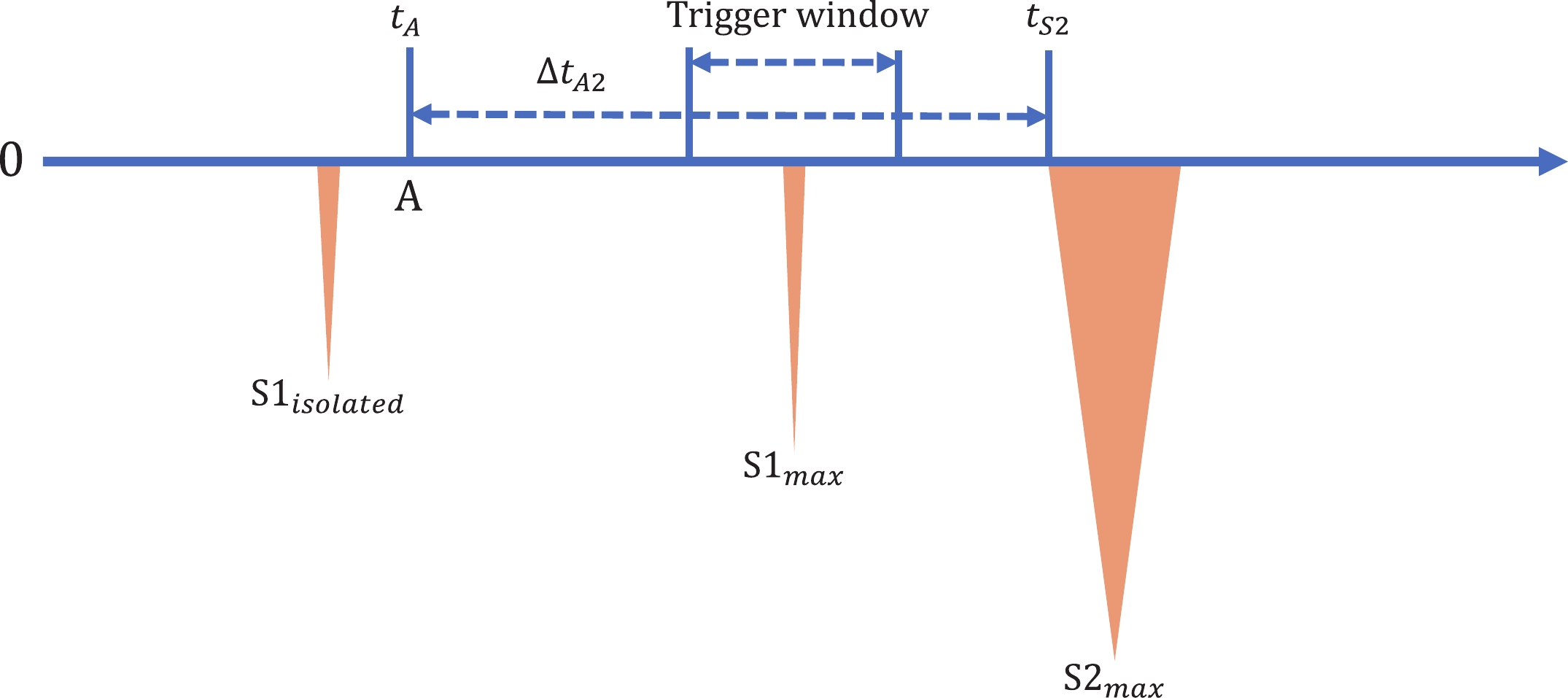
Figure 4. (color online) Schematic view on the search of isolated
$ S 1 $ in events triggered by$ S 1 $ ($ S1_{\rm max} $ ) in Runs 10 and 11.In this method, the rate
$ r_1 $ in a data taking period can be estimated as$ \begin{equation} r_1 = \frac{n_{iS 1}}{ \sum{(t_{S 2} - \Delta t_{A2}})}, \end{equation} $

(5) where
$ n_{iS 1} $ is the total number of isolated$ S 1 $ . The variables of time are defined in each of the good events, with$ t_{S 2} $ as the start time of the$ S 2 $ signal relative to the start of the event, and$ \Delta t_{A2} $ as the size of the exclusion window, which takes the same value as the maximum drift time.We studied the distribution of time difference
$ \Delta t $ between the isolated$ S 1 $ and the good$ S 1 $ , as shown in Fig. 5. Considering the uniformity separation of the physical$ S 1 $ and$ S 2 $ signals, the requirement of the isolated$ S 1 $ outside the maximum drift window reduces the probability of isolated$ S 1 $ s with a small$ \Delta t $ being selected. Because the selection window is reduced in the same time, the rate calculation is not affected. This behavior is reproduced with a simple toy MC simulation by randomly sampling$ S 2 $ after the triggered$ S 1 $ in the drift window and randomly sampling isolated$ S 1 $ in the whole event window, especially for Run 9. The same MC simulation can also be used to verify the rate calculation. Assuming the rate of isolated$ S 1 $ is 500 Hz, the rate calculated with method 3 is$ 498.9 $ Hz, showing a good accuracy. For Run 10, this behavior is not visible owing to the relative low statistics of the isolated$ S 1 $ . For Run 11, excess isolated$ S 1 $ s ($ 11.6\% $ ) are observed for$\Delta t < 120$ μs, which are found in the events accumulated in the cathode region, as illustrated in Fig. A1 in Appendix A. The origin of these signals is still unknown.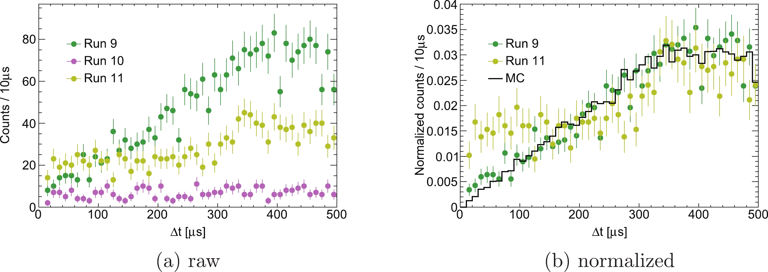
Figure 5. (color online) Distribution of the time difference
$ \Delta t $ between the isolated$ S 1 $ and triggered$ S 1 $ in method 3. (a) Raw distribution. (b) The integration of the distribution is normalized to 1.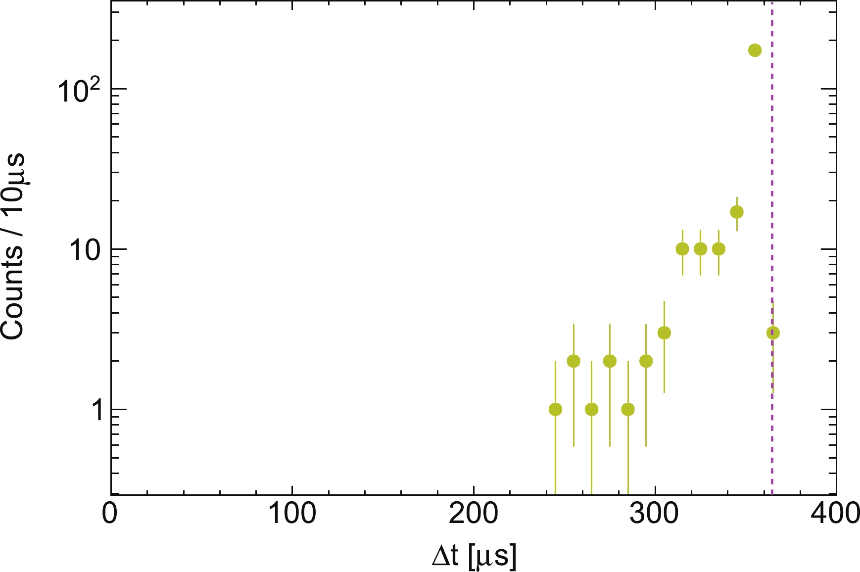
Figure A1. (color online) Distribution of the time difference between
$ S 1_{\rm max} $ and$ S 2_{\rm max} $ at the condition where time difference between the isolated$ S 1 $ and$ S 1_{\rm max} $ is smaller than 120 μs ($ \Delta t < 120 $ μs) in method 3. The pink dashed line represents the maximum drift time. -
The estimation of the rate
$ r_2 $ for isolated$ S 2 $ is more straightforward in comparison with isolated$ S 1 $ . The events triggered by unpaired$ S 2 $ , with all the related quality cuts applied, are selected to calculate the rate. The rate is defined as$ r_{2} = \frac{n_{iS 2}}{T}, $

(6) where
$n_{iS 2}$ is the number of events that satisfy the selection criteria, and T is the duration of the run. -
The estimated average rates of isolated
$ S 1 $ and$ S 2 $ in each run are presented in Table 1. Run 9 has the highest rate of isolated$ S 1 $ , which is very likely to be attributed to the higher dark rate of PMTs operating with a higher gain [5]. For Runs 10 and 11, the$ \bar{r}_1 $ values calculated with methods 1 and 3 are consistent with each other within uncertainty. The results of method 3 are used in the final analysis of PandaX-II [4] and in the rest of this study to estimate the rate of accidental background. The variance of the average rates of isolated$ S 2 $ is small.Run Duration/d $ \bar{r}_1 $ /Hz

$ \bar{r}_2 $ /Hz

Method 1 Method 2 Method 3 9 79.6 − $ 1.40\pm0.25 $ 

$ 1.53\pm0.16 $ 

$ 0.0121\pm0.0002 $ 

10 77.1 $ 0.46\pm0.05 $ 

$ 0.27\pm0.20 $ 

$ 0.47\pm0.02 $ 

$ 0.0130\pm0.0007 $ 

11 244.2 $ 0.77\pm0.06 $ 

$ 0.37\pm0.16 $ 

$ 0.69\pm0.06 $ 

$ 0.0121\pm0.0001 $ 

Table 1. Average rates of isolated
$ S 1 $ and$ S 2 $ extracted from PandaX-II data. The results from method 2 have been corrected by subtracting the contamination from the possible 214Bi-214Po cascade decay signals.A more detailed evolution of the rates of the isolated signals during the whole PandaX-II data taking period, with those of isolated
$ S 1 $ calculated by method 3, is presented in Fig. 6. The rate of isolated$ S 2 $ remains stable, while that of isolated$ S 1 $ varies greatly. The large variance of$ r_1 $ in Run 9 might come from the occasional sparking of electrodes or PMTs. A peak rate of isolated$ S 1 $ is observed in Run 11, which can be explained by the fact that some PMTs were unstable during the corresponding period, as shown in Fig. A2 in Appendix A. The ordinary data quality cut cannot remove related events efficiently.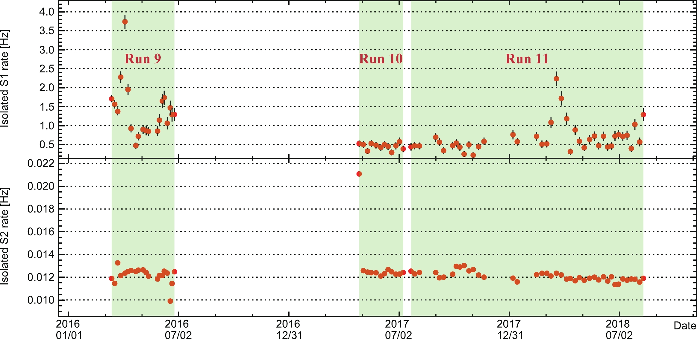
Figure 6. (color online) Evolution of rates of the isolated signals during the whole PandaX-II data taking period, selected by method 3.

Figure A2. (color online) Accumulated charge pattern in the top PMT array of all isolated S1s from Mar. 11, 2018 to Apr. 6, 2018. Three PMTs are observed to have the largest contribution to these signals.
The charge spectra of the isolated signals selected by method 3 are shown in Fig. 7. Most of the isolated
$ S 1 $ are found to be smaller than 10 PE. All of the$ S 1 $ spectra have a similar shape when the charge is larger than 6 PE, but a higher peak is observed below 6 PE for Run 9. This may be explained by the higher chance of accidental coincidence of hits from dark current in this run due to the higher operation voltage of the PMTs. A small peak in Run 11 around 10 PE results from the unstable PMTs mentioned before (see Fig. A3 in Appendix A). The spectra of isolated$ S 2 $ are consistent with each other.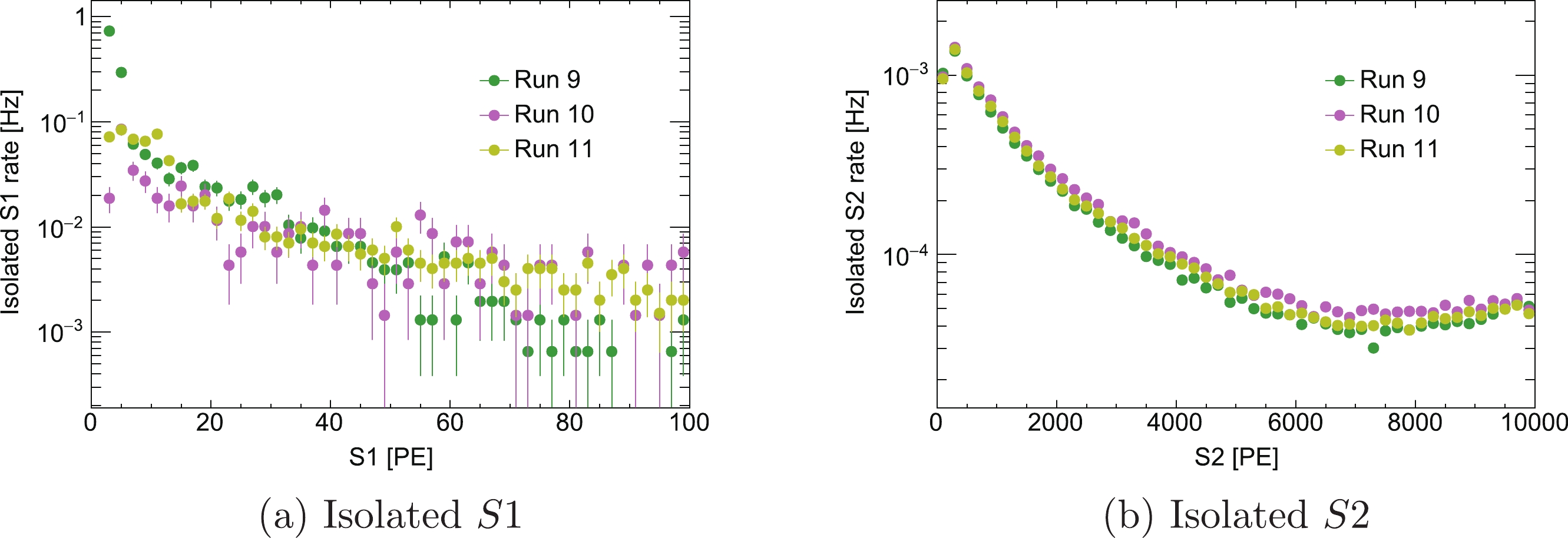
Figure 7. (color online) Charge spectra of isolated signals selected by method 3.
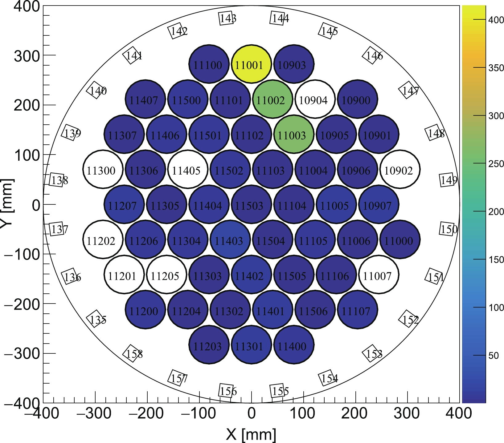
Figure A3. (color online) Accumulated charge pattern in the top PMT array of isolated S1s in the window of
$ (10, 12) $ PE in Run 11. Three PMTs are observed to have the largest contribution to these signals. -
A data-driven MC simulation with the selected isolated signals is used to study the accidental background events. For each run, the isolated
$ S 1 $ and$ S 2 $ are paired randomly, with the time separation between them sampled uniformly in the time window$ \Delta t_w $ defined by the fiducial volume cut. The horizontal position of the event is determined by the$ S 2 $ signal. The paired mock event is treated as an event with raw signals. The same position-dependent charge corrections and quality cuts for dark matter search data are applied to these events, resulting in a cut efficiency$ \epsilon $ .Then, the total number of accidental background events
$ n_{\rm{acc}} $ can be calculated by$ \begin{equation} n_{\rm{acc}} = \bar{r}_1\cdot \bar{r}_2 \cdot \Delta t_{w} \cdot T \cdot \epsilon. \end{equation} $

(7) The efficiency
$ \epsilon $ , the total number of accidental events, and the number of events below the median line of the NR band from calibration data [4] results, are presented in Table 2. Run 11 has the largest number of accidental background events because it has the largest duration T.Run Type $ \epsilon $ 

$ n_{\rm{acc}} $ 

9 total 21.9% $ 8.15\pm0.94 $ 

below NR median 3.5% $ 1.31\pm0.15 $ 

10 total 25.6% $ 3.16\pm0.15 $ 

below NR median 8.5% $ 1.06\pm0.05 $ 

11 total 18.2% $ 9.87\pm0.89 $ 

below NR median 5.6% $ 2.93\pm0.27 $ 

Table 2. Number of accidental events estimated with the selected isolated signals using method 3.
The distributions of
$ \log_{10}(S 2/S 1) $ vs.$ S 1 $ for the simulated accidental background events after all the quality cuts within the dark matter search window [4] are given in Fig. 8, together with those of the NR calibration data. Most of the accidental events have a relatively small$ S 1 $ charge and are above the NR median. Considering the low statistics of the most critical ER backgrounds below the NR median, the non-negligible accidental background in this region will reduce the discovery power for WIMPs. Suppressing these background events could improve the sensitivity of the detector for WIMP search.
Figure 8. (color online) Distribution of
$ \log_{10}(S 2/S 1) $ vs.$ S 1 $ for the simulated accidental background and NR calibration data. The red curves are the corresponding NR median for each run. -
The accidental events are composed of isolated
$ S 1 $ and$ S 2 $ . Since there is no physical correlation between the two signals, we would expect there to be a method that is able to distinguish them from the physical events by considering the joint distributions of the properties of these signals. However, because all of the selected accidental events have passed the quality cuts, it is difficult to differentiate between any single property of the signals from accidental and physical events. A multi-variant analysis can be a possible solution. The BDT algorithm, one of the most successful multi-variant analysis methods used in particle physics [18], was first used to suppress the accidental background in the first analysis results of PandaX-II [6]. The real signal of the WIMP-nucleon scattering is NR, thus the single scattering events from NR calibration runs (AmBe) should be used as input signals in machine learning, with randomly paired events as backgrounds. Given the fact that the ER events dominate the region above the NR median in the dark matter search data and the relatively low estimated number of accidental events in the region, we only distinguish the accidental background from the physical NR events below the NR median. -
The TMVA (Toolkit for Multivariate Data Analysis) package in ROOT is used to perform the BDT machine learning [19]. A set of signal properties are exploited to search for the difference between the accidental events and the physical NR events, including:
● corrected charge of
$ S 1 $ (qS1);● corrected charge of
$S 2$ (qS2);● raw charge of
$S 1$ (qS1R);● raw charge of
$S 2$ (qS2R);● width of
$S 2$ (wS2);● full width at tenth maximum of
$S 2$ (wTenS2);● asymmetry between the top and bottom charges for
$S 1$ (S1TBA);● ratio of the top charge to the bottom charge for
$S 2$ (S2TBR);● the ratio of the pre-max-height charge to the total charge of an
$S 2$ signal (S2SY1 in the directly summed over waveform, S2SY2 in the smoothed waveform);● number of local maximums (peaks) of
$S 1$ (S1NPeaks);● ratio of the largest charge collected by the bottom PMT of
$S 1$ to total charge of S1 (S1LargestBCQ).The distributions of the these variables for the events below the NR median can be found in Fig. 9, and their correlations are presented in Fig. A5.

Figure 9. (color online) Distribution of the selected variables from the NR calibration data (signal) and the simulated accidental events (background) in Run 11. Only the events below the NR median were selected.

Figure A5. (color online) Correlations between the variables used for BDT training, from the events below the NR median.
-
We constructed the adaptive BDT using the default parameters provided by the official ROOT TMVA classification example, except the parameter of
$\texttt{NTrees}$ (number of trees). We trained the data for the three runs independently, each with a predefined set of$\texttt{NTrees}$ . After the training, the resulted BDT response distributions of the training and test data samples were superimposed, and the Kolmogorov-Smirnov (K-S) test was performed to check for overtraining (see Fig. A4 for details). We chose$\texttt{NTrees} =90 $ for further study. With the trained BDT, the "likelihood" estimators can be calculated for an input event to be classified. The best cut criterion for the estimator was obtained with the test data set by maximizing the significance S,
Figure A4. (color online) The distributions of BDT response of the train and test data samples. The K-S test probabilities are used to indicate the overtraining.
$ S = \frac{\epsilon_s n_s}{\sqrt{\epsilon_s n_s + \epsilon_b n_b}}, $

(8) where
$ n_s $ and$ n_b $ are the number of signal and background events, respectively, and$ \epsilon_s $ and$ \epsilon_b $ are the efficiencies for signal and background events at a given estimator value, respectively. In this study, the expected signal events below the NR median are likely to be the neutron background or the WIMP events, and they are estimated at the same level as the accidental background [4]. Therefore, the identical numbers$ n_s $ and$ n_b $ are used to calculate the significance. The evolution of the background rejection efficiency with the signal efficiency at different BDT cut values is shown in Fig. 10. The results at the maximum significance S are presented in Table 3. The BDT algorithm is able to remove$ 70\% $ of the accidental background events, while keeping about$ 90\% $ of the single scattering NR events below the NR median curve in all of the three runs. The distributions of the BDT cut efficiency on the$ \log_{10}(S 2/S 1) $ vs.$ S 1 $ plane for the simulated accidental background are shown in Fig. 11.
Figure 10. (color online) The evolution of the background rejection efficiency with the signal efficiency at different BDT cuts for different runs. The initial numbers of background and signal events are assumed to be identical.
Run S $ \epsilon_s $ 

$ 1-\epsilon_b $ 

9 25.9 90.4% 70.2% 10 26.5 91.1% 74.6% 11 26.2 90.7% 73.7% Table 3. The significance S, signal efficiencies
$ \epsilon_s $ , and background rejection efficiencies$ 1-\epsilon_b $ at the best cut value of the estimator for events below the NR median lines, assuming$ n_s=n_b $ .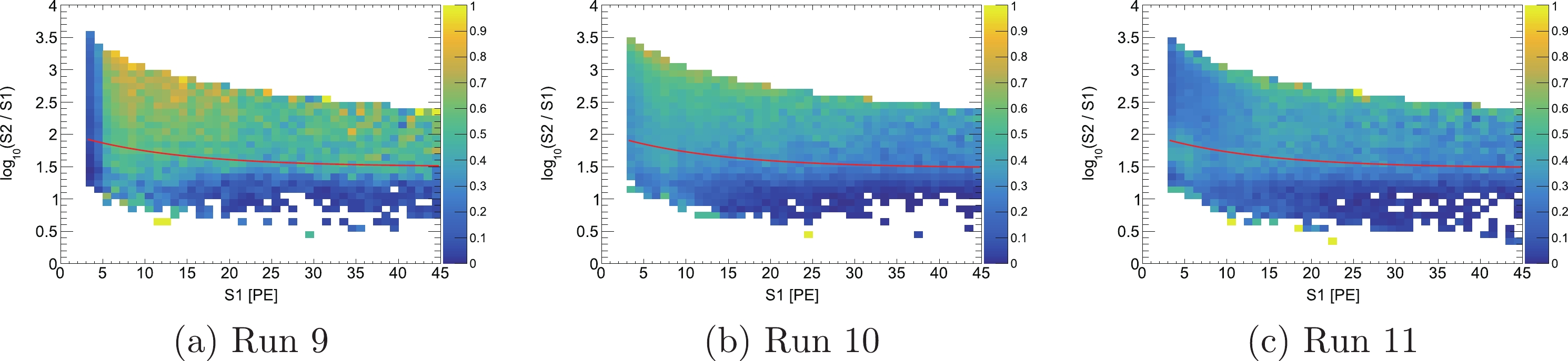
Figure 11. (color online) BDT cut efficiency map on the
$\log_{10}(S 2/S 1)$ vs.$S 1$ distribution for the simulated accidental background.The contribution of each input variable to the discrimination power is extracted by the BDT training. The variables wS2, S2SY2, and S1TBA are found to be the most critical to the recognition of accidental backgrounds. By checking the distributions of these variables, isolated
$ S 2 $ signals are found to have a smaller width (wS2) and more asymmetrical shape (S2SY2) in comparison with those in normal events, indicating that most of these signals are generated near the grid wires [20]. The peak in the S1TBA distribution of physical events at the value of -1 suggests a large fraction of the physical$ S 1 $ signals have no hits on the top PMT array. Given the fact that physical$ S 1 $ s are produced inside the liquid xenon, small signals have a smaller chance of being detected by the top PMTs due to the total reflection on the surface between the liquid and gas xenon. However, some of the non-physical$ S 1 $ s are from the coincidence of dark noises on top PMTs, resulting in a S1TBA larger than -1. The distribution of S1TBA could be used to estimate the fraction of isolated$ S 1 $ s from the coincidence of dark noise on top PMTs. This phenomenon helps to distinguish the non-physical small$ S 1 $ signals from the real ones. -
In the analysis, the BDT cut is applied to not only the events below the NR median but to all events in the search window. The efficiencies of BDT for different types of events are extracted by using the calibration data sets, shown in Fig. 12. The BDT cut efficiencies for the ER and NR calibration data, expressed as functions of
$ S 1 $ , are used to build the final signal model [21]. The efficiencies for ER events are lower than those of NR events when$ S 1<8 $ PE, in all of the data set. From the 2D efficiency maps, it is observed that in the region of low$ S 1 $ , the ER events with a higher ratio of$ S 2/S 1 $ are suppressed heavily in Runs 10 and 11. On the contrary, more ER events with smaller$ S 2/S 1 $ in the same region are suppressed in Run 9. The different distributions of$ S 2 $ related variables of the different ER calibration data may result in the different efficiencies. The distributions of$ \log_{10}(S 2/S 1) $ vs.$ S 1 $ of accidental background after the BDT cut are used directly in the model.
Figure 12. (color online) The BDT cut efficiency curves as a function of
$ S 1 $ and efficiency maps on the$ \log_{10}(S 2/S 1) $ versus$ S 1 $ for different calibration data in the dark matter search window for different runs.The expected numbers of accidental background (below NR median) in the PandaX-II full exposure data set after the BDT cuts are
$ 2.09\pm0.25 $ ($ 0.39\pm0.05 $ ),$ 1.03\pm0.05 $ ($ 0.27\pm0.01 $ ), and$ 2.53\pm0.24 $ ($ 0.77\pm0.07 $ ) for Runs 9, 10, and 11, respectively. The total number of expected accidental background events below the NR median is smaller than 1.5. Considering that the total data taking period of PandaX-II is 244.2 days, we have successfully suppressed the accidental background to a trivial level and improved the final sensitivity for dark matter search [4]. -
The accidental background is an important composition of the backgrounds in the dark matter search experiments with a dual phase xenon detector. In this study, we discussed the possible origins of the two components, isolated
$ S 1 $ and$ S 2 $ , and developed methods to estimate the level of accidental background in the PandaX-II experiment. The BDT algorithm is used to distinguish this non-physical background from real NR signals below the NR median lines, so that the level of this background is suppressed greatly.We found that the rate of isolated
$ S 1 $ is much higher in Run 9, during which the PMTs run with higher gains than in other runs. This suggests the coincident combination of hits created by dark noise contributes to a large amount of the isolated$ S 1 $ . Thus, reducing the dark noise of PMTs is critical for next generation of experiments [22–24].The BDT method works well in the suppression of the accidental background in our study. The analysis framework and suppression method can be used in the data analysis of the subsequent PandaX-4T experiment [25]. Because the number of accidental events is nearly proportional to the operation time, only a few of them have been produced in the commissioning run, and have been suppressed to a very low level with the quality cuts. Therefore, this method is not used in the first PandaX-4T WIMP search. However, PandaX-4T and other similar experiments will be running much longer than PandaX-II, and our study provides a valuable reference for them. With the rapid development of machine learning methods in recent years, we may expect neural networks or other machine learning algorithms to achieve equivalent success in this topic.
-
We are grateful for the support from the Double First Class Plan of the Shanghai Jiao Tong University. We are also thankful for the sponsorship from the Chinese Academy of Sciences Center for Excellence in Particle Physics (CCEPP), Hongwen Foundation in Hong Kong, and Tencent Foundation in China. Finally, we thank the CJPL administration and the Yalong River Hydropower Development Company Ltd. for indispensable logistical support and other assistance.
Study of background from accidental coincidence signalsin the PandaX-II experiment
- Received Date: 2022-06-22
- Available Online: 2022-10-15
Abstract:


 DownLoad: