QED effects on phase transition and Ruppeiner geometry of Euler-Heisenberg-AdS black holes

Since the earliest pioneering work of Hawking and Bekenstein on the temperature and entropy of black holes, it has been revealed that there is a deep connection between gravity, quantum mechanics, and thermodynamics [1–3]. Equipped with the established four laws of black hole thermodynamics [4], the study of thermodynamics has become an increasingly active area in black hole physics. Motivated by anti-de Sitter/conformal field theory (AdS/CFT) correspondence [5, 6], the Hawking-Page phase transition [7] between a stable large Schwarzschild AdS black hole and thermal space has been interpreted as the confinement/deconfinement phase transition of the gauge field [8]. The phase transition was also extended to charged and rotating AdS black hole cases [9–11].

Recently, it was found that, by interpreting the cosmological constant as thermodynamic pressure in AdS space [12–14], black hole systems are analogous to everyday thermodynamic systems. In this extended thermodynamic phase space, the charged small/large AdS black hole phase transition is similar to the gas-liquid phase transition of van der Waals (VdW) fluids [15]. Subsequently, additional interesting black hole phase transitions and phase structures, such as the reentrant phase transition [16, 17], isolated critical point [18], triple point [19–21], and superfluid black hole phase [22], have been uncovered. Now, this field is known as black hole chemistry, which aims at uncovering the similarity and differences between black hole systems and everyday thermodynamic systems.

Understanding the black hole microstructure is a significant challenge. Although string theory [23–26], the fuzzy ball model [27, 28], and pierced horizons [29] have made great progress, more questions remain unanswered. As proposed in Refs. [30, 31], the study of black hole phase transition can also be applied to this challenge with the assumption that the micro-degree of freedom is measured by the underlying molecules of the black hole. Combined with Ruppeiner geometry [32], the characteristic black hole microstructure has been tested. The scalar curvature of its corresponding geometry is an important tool for exploring the microstructure of a black hole, and empirical observation has shown that the positive or negative scalar curvature corresponds to the repulsive or attractive interaction among these underlying black hole molecules. Such empirical results have been supported by numerous studies on different fluid systems, such as ideal fluids [33], VdW fluids [34], one-dimensional Ising models, and quantum gases [35, 36]. More significantly, when considering a microscopic model and the equation of state, a possible interpretation of the empirical observation was given and the corresponding molecular potential was constructed in Ref. [37].

In view of the "hard-core" model, there is only a dominant attractive interaction for the VdW fluid. However, for charged AdS black holes, a dominant repulsive interaction emerges for a small black hole (SBH) with a high temperature [38], which uncovers an interesting phenomenon for the black hole microstructure. After generalizing the study for the modified gravity [39], it was found that the dominant repulsive interaction may not emerge, whereas the attractive interaction is universal. Other related studies can be found in Refs. [40, 41].

Although quantum gravity remains to be established, understanding of black hole microstates can be classically tested using the Ruppeiner geometry of AdS black holes. Inspired by the AdS/CFT correspondence, Ruppeiner geometry may be relevant to dual CFT. In particular, there have been studies in which the change in the pressure or cosmological constant of the bulk was considered to correspond to the change in the number of colors in the boundary of Yang-Mills theory. Ruppeiner geometry was also constructed in Refs. [42–45], and many interesting properties were found. More recent developments on this issue also focused on thermodynamic laws and phase transitions in dual field theory by combining cosmological and Newton constants as well as the central charge [46–48].

Furthermore, black hole solutions with nonlinear electrodynamics have been gaining great interest. In particular, this theory can be viewed as a low-energy limit from string theory or D-brane physics, where Abelian and non-Abelian nonlinear electrodynamic Lagrangians can be produced. The thermodynamics of charged Born-Infeld (BI) AdS black holes were considered in Ref. [49]. The presence of BI vacuum polarization governs a rich black hole phase transition. The study was also extended to higher dimensions, and the SBH/large black hole (LBH) phase transition was found to be universal [50]. Another widely concerned nonperturbative one-loop effective Lagrangian of nonlinear electromagnetic fields was proposed by Heisenberg and Euler [51] and reformulated within the QED framework by Schwinger [52]. The black hole solutions corresponding to the effective Lagrangian have been calculated [53]. In Refs. [54–58], the first law of black hole thermodynamics and the Smarr formula were found to be consistent with each other when the vacuum polarization parameter is included. The phase transition was preliminarily studied, and at the critical point, the standard mean field theory exponents were obtained.

Motivated by this, in this paper, we thoroughly study the phase transition of charged Euler-Heisenberg (EH)-AdS black holes by considering the QED effect. The SBH/LBH phase transition and reentrant phase transition are found to exist in different regions of the parameter space. The phase diagrams and structures are shown in their entirety. Then, based on the phase diagrams, we construct the Ruppeiner geometry of charged EH-AdS black holes. The feature of scalar curvature is also obtained. Furthermore, employing the empirical observation of the Ruppeiner geometry, we disclose a particularly interesting property of the microstructure of black holes.

This paper is organized as follows. In Sec. II, we first review the thermodynamics of charged EH-AdS black holes. Then, in different regions of the parameter space, we study the SBH/LBH phase transition and reentrant phase transition. The phase diagrams are clearly exhibited. In Sec. III, Ruppeiner geometry is constructed. Employing the corresponding scalar curvature, we explore the characteristic black hole microstructure under the SBH/LBH phase transition and reentrant phase transition. Novel properties are found. Finally, the conclusions and discussions are given in Sec. IV.

In this section, we briefly review the thermodynamics of charged EH-AdS black holes with QED correction [53] and then study their phase transition in complete parameter space, where the SBH/LBH phase transition and reentrant phase transition are clearly exhibited.

The action of EH theory with a cosmological constant in four-dimensional spacetime is [59]

Here, g, Λ, and R are the determinant of the metric tensor, cosmological constant, and Ricci curvature tensor, respectively. The term $\mathcal{L}(F,G)$ is the Lagrangian of nonlinear electrodynamics, which depends on the electromagnetic invariants $F=\dfrac{1}{4}F_{\mu\nu}F^{\mu\nu}$ and $G=\dfrac{1}{4}F_{\mu \nu}{^*F^{\mu \nu}}$. The symbol $F_{\mu \nu}=\partial_{\mu}\mathcal{A}_{\nu}-\partial_{\nu}\mathcal{A}_{\mu}$ denotes the electromagnetic field tensor, and $^\ast F^{\mu\nu}=\epsilon_{\mu\nu\sigma\rho}F^{\sigma\rho}/(2\sqrt{-g})$ is its dual, where $\mathcal{A}_{\mu}$ is the corresponding vector potential. The parameter a in Eq. (2) can be used to measure the strength of the QED correction, which is related to the mass and charge of an electron, and thus we call it the QED parameter. When a=0, the influence of the QED term vanishes.

For a static spherically symmetric charged EH-AdS black hole solution, the line element is [56]

and the metric function $f(r)$ is given by

where M and Q are the mass and electric charge of the black hole, respectively. When $a=0$, this solution reduces to the Reissner-Nordström (RN) AdS black hole solution. The EH electromagnetic potential $\Phi(r)$ and electric field of EH-AdS black holes are given by [56]

Similar to the electric field behavior of a point charge in Maxwell's linear electromagnetic theory, the electric field $\mathcal{E}(r)$ diverges at $r=0$. However, the Maxwell behavior is recovered when $a=0$.

The radius $r_+$ of the outer black hole event horizon is the largest root of $f(r_+)=0$, which can be obtained by solving

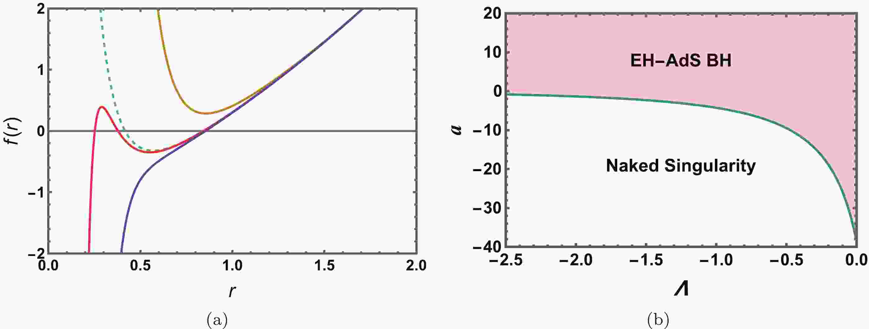
The radius $r_+=r_+(M,Q,\Lambda,a)$ of the event horizon of an EH-AdS black hole depends on four parameters: the mass M, electric charge Q, cosmological constant Λ, and QED parameter a. In different parameter regions, there may be two, one, or no horizons. Taking $Q=0.8$, $M=1.0$, and $\Lambda=-2<0$ as an example, we plot the metric function $f(r)$ in Fig. 1(a) for $a=-5$, $0$, $0.04$, and $0.4$. We observe that when $a<-5$, there is no black hole horizon, and only one naked singularity is present. For a=0, 0.04, and 0.4, there are two, three, and one horizons, respectively. Therefore, we may conclude that there is no horizon for $a<0$, whereas at least one horizon exists for $a\geq0$.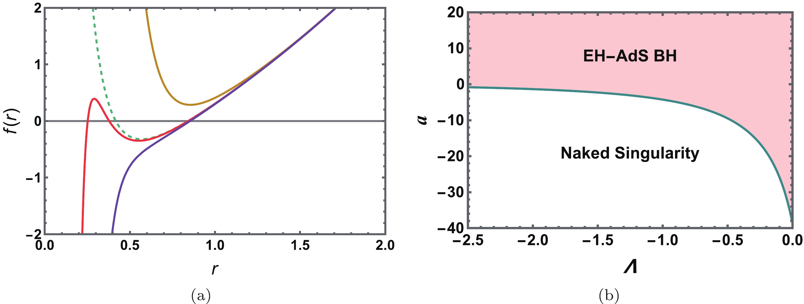

Figure 1.  (color online) (a) Metric $f(r)$ of an EH-AdS black hole for parameters $\Lambda=-2$ and $a=-5$, $0$, $0.04$, and $0.40$ from top to bottom. (b) Parameter regions for the EH-AdS black hole and naked singularity in the (a, Λ) plane with $M=1$ and $Q=0.8.$

To clearly show whether there is black hole horizon, we examine the asymptotic behavior of the metric $f(r)$ (4) at $r\to 0$ and $r\to \infty$. Expanding this, we obtain

Considering that in AdS space, Λ is negative, one can reach $f(r)\to \infty$ as $r\to \infty$. Near $r\to 0$, $f(r)$ tends to positive infinity for $a<0$ and negative infinity for $a>0$. Hence, for the case of $a>0$, we can find $r_* \in [0,\infty]$ such that $f(r_*)=0$ according to the intermediate value theorem. Therefore, there is at least one black hole horizon at $r=r_*$ for $a>0$. For negative a, the behaviors of $f(r)$ are obscure. A naked singularity may emerge in some parameter regions. As an explicit example, we show the regions for the naked singularity and black hole on the (a, Λ) plane (see Fig. 1(b)) with $M=1$ and $Q=0.8$. The solid curve represents black holes with one degenerated horizon. Above and below the curve are the black hole and naked singularity regions, respectively. It is clear that the entire positive a region is for the black hole. Moreover, we find that, with increasing Λ, the parameter region of a increases for the black hole. A similar pattern also holds for other values of the black hole charge Q.

In terms of $r_+$, the mass M from (7) can be expressed as

Using the “Euclidean trick,” the Hawking temperature is

In the extended phase space, the cosmological constant Λ is interpreted as the pressure using ${P}=-\dfrac{\Lambda}{8\pi}$ [12]. Accordingly, the black hole mass M acts as the enthalpy H of the thermodynamic system, rather than the internal energy. Then, the first law has the following form:

where $\mathcal{A}=\dfrac{\partial H}{\partial a}$ is the conjugate quantity of the QED parameter a. The entropy S, thermodynamic volume V, electric potential Φ, and $\mathcal{A}$ can be calculated using

It is straightforward to confirm that the following Smarr formula holds:

From Eq. (11), the equation of state can be written as

This equation of state reveals more than one critical point, which can be determined by the following conditions:

These conditions give a third degree equation for $x=\left(6V/\pi\right)^{2/3}$

When $0\leq a \leq \dfrac{32}{7} Q^2$, Eq. (20) has three real roots [56],

Note that $x_2$ gives a negative volume and should be excluded. Therefore, only k=0 and 1 are allowed, and the critical temperature and pressure are given by

The critical volume is defined as $V_c=\dfrac{1}{6} \pi x_{k}^{3/2}$, depending on the charge Q and QED parameter a. It is worth noting that when the QED parameter $a > \dfrac{32 Q^2}{7}$, Eq. (20) has no real root, and thus no critical point exists. For $a<0$, there is a real root $x_0$ (k=0), which gives one critical point.

To clearly show the number of critical points, we plot $F(x)=x^3-24Q^2x^2+448aQ^4$ as a function of x in Fig. 2 with Q=1. The zero points marked with black dots simply correspond to the solution of Eq. (20), and thus they are the critical points of concern. It is worth noting that the parameter $x>0$. For different values of a, $F(x)$ has a similar pattern. We also observe that for $a<0$, there is only one zero point located near x=25. With an increase in a such that $a=0$, a second zero point emerges near $x=0$. By further increasing a, these two zero points approach and coincide near $x=16$ for $a=32/7$. Beyond this, the zero point disappears. As a result, such behavior is entirely consistent with the above discussion on the critical point.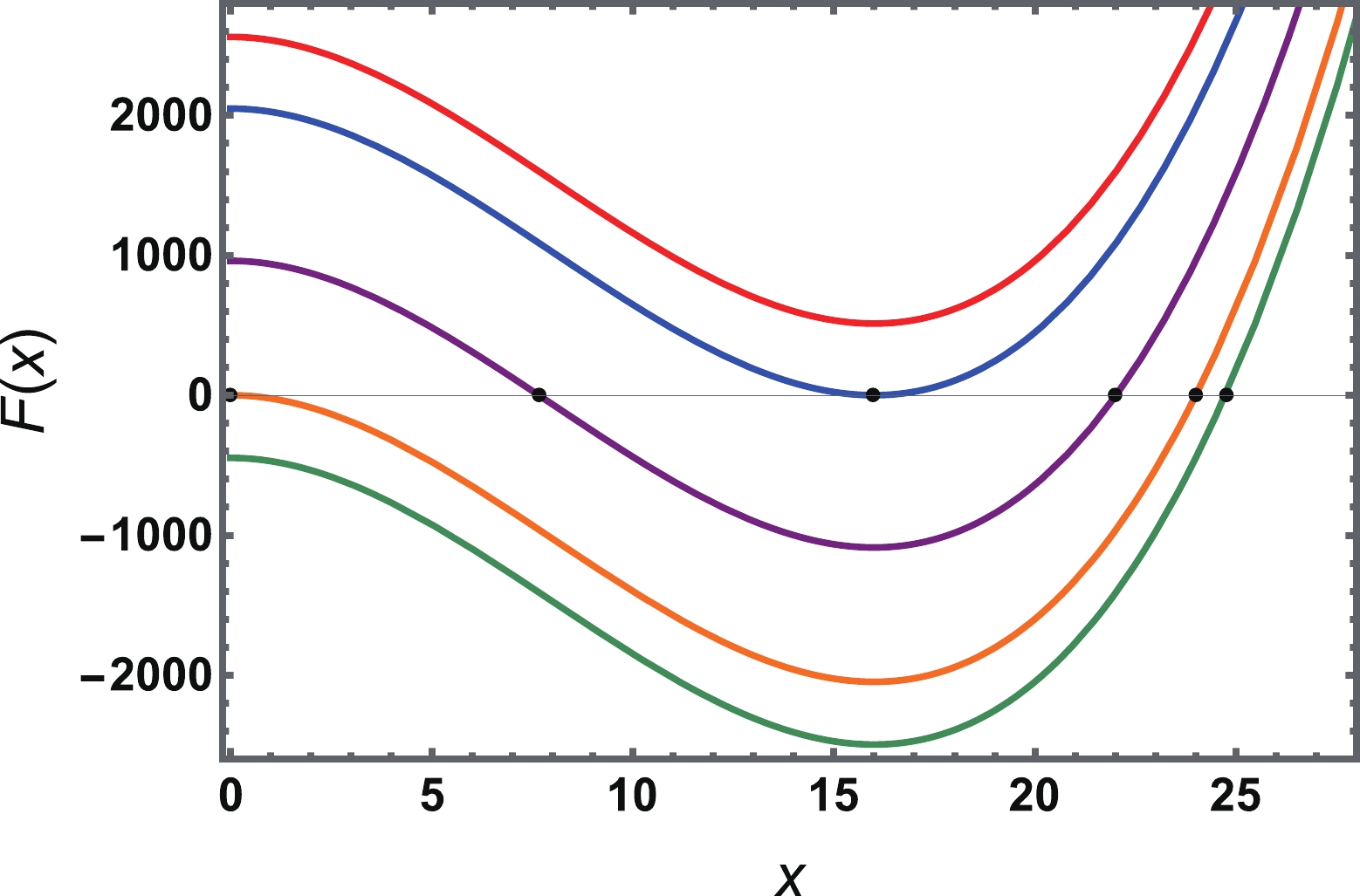

Figure 2.  (color online) Behavior of $F(x)$ as a function of x. The QED parameter a=${40}/{7}$ (red), ${32}/{7}$ (blue), ${15}/{7}$ (purple), 0 (orange), and –1.0 (green) from top to bottom. Note that the zero points (marked with black dots) of the function $F(x)$ are the critical points. The charge Q is set to one.

In summary, there are two characteristic types of phase transitions. The first type is for $a<0$, which reveals one critical point, and this phase transition is similar to the gas-liquid phase transition of VdW fluids. For the other type, with the QED parameter $0 < a < \dfrac{32 Q^2}{7}$, two critical points can be found, and the reentrant phase transition exists.

For these two types of phase transitions, we may recognize differences from the equation of state (18) expressed in terms of the thermodynamic volume $V=\dfrac{4}{3}\pi r_+^{3}$,

We plot the pressure P as a function of the specific volume $v=2\, r_+$ for fixed temperature in Fig. 3 with $a=-1.5$ ($a<0$) and $a=1.0$ ($0 \leq a \leq \dfrac{32}{7}Q^2$) as two representative examples. In Fig. 3(a), there are two extremal points (marked with red dots) for $T<T_c$, and these points divide the isothermal curve into three branches. Two of them are the SBH and LBH located at the left and right sides of the isothermal curve, respectively, whereas the middle branch is for the intermediate black hole. According to the heat capacity, black hole branches with a negative slope are thermodynamically stable, whereas those with a positive slope are unstable. Thus, the SBH and LBH are stable, whereas the intermediate black hole is unstable. Making use of Maxwell's equal area law, we can construct two equal areas along each isothermal curve to obtain the phase transition point. However, with increasing temperature, these two extremal points get closer and coincide at $T=T_c$. When $T>T_c$, there is no longer any extremal point. In contrast, for a positive QED parameter, i.e., $a=1.0\in(0 \leq a \leq \dfrac{32}{7}Q^2)$, there are three extremal points in Fig. 3(b) for $T<T_c$. When the temperature approaches its critical value, two of them coincide, whereas the other one continues to exist, even when the temperature is above the critical value. Below the critical temperature, the nonmonotonic behavior of the isothermal curve also allows us to construct two equal areas, indicating the existence of the black hole phase transition.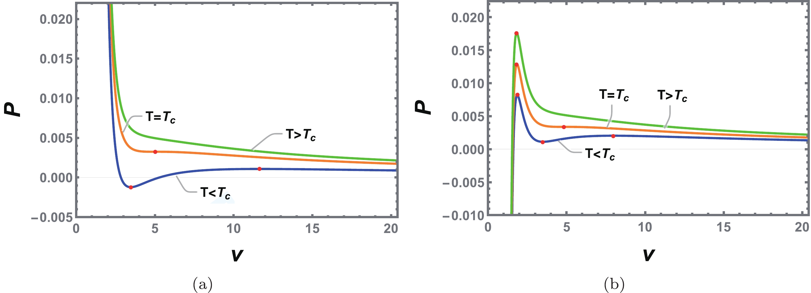

Figure 3.  (color online) Isothermal curves on the P-v plane of the charged EH-AdS black hole. (a) $a=-1.5$ ($a<0$). (b) $a=1.0$ ($0 \leq a \leq \frac{32}{7}Q^2$). The temperature $T<T_c$, $T=T_c$, and $T>T_c$ from bottom to top. The extremal points are marked with red dots, and we set $Q=1$.

For convenience of discussion, we can introduce the reduced quantities ${\tilde{P}}$, ${\tilde{T}}$, ${\tilde{V}}$, and ${\tilde{v}}$ in the extended phase space.

Then, the equation of state (23) takes the following form:

where $\rho_c=\dfrac{P_{c}v_{c}}{T_c}$. In the canonical ensemble, the Gibbs free energy $G=H-TS$, which reads

In general, the first-order phase transition can be determined by the swallow tail behavior of the Gibbs free energy. In the following sections, we study the phase transition via the behavior of the Gibbs free energy.

For this case, we take $Q=1.0$ and $a=-1.5$ as an example. The Gibbs free energy G is plotted with the temperature T in Fig. 4 for different values of pressure. When $P<P_c$, we observe the characteristic swallow tail behavior, indicating the coexistence of the black hole phase transition. As the pressure increases, the shape of the swallow tail becomes smaller and shrinks to a point when $P=P_c$. By further increasing the temperature, the behavior completely disappears. Then, the Gibbs free energy turns into a smooth function of temperature.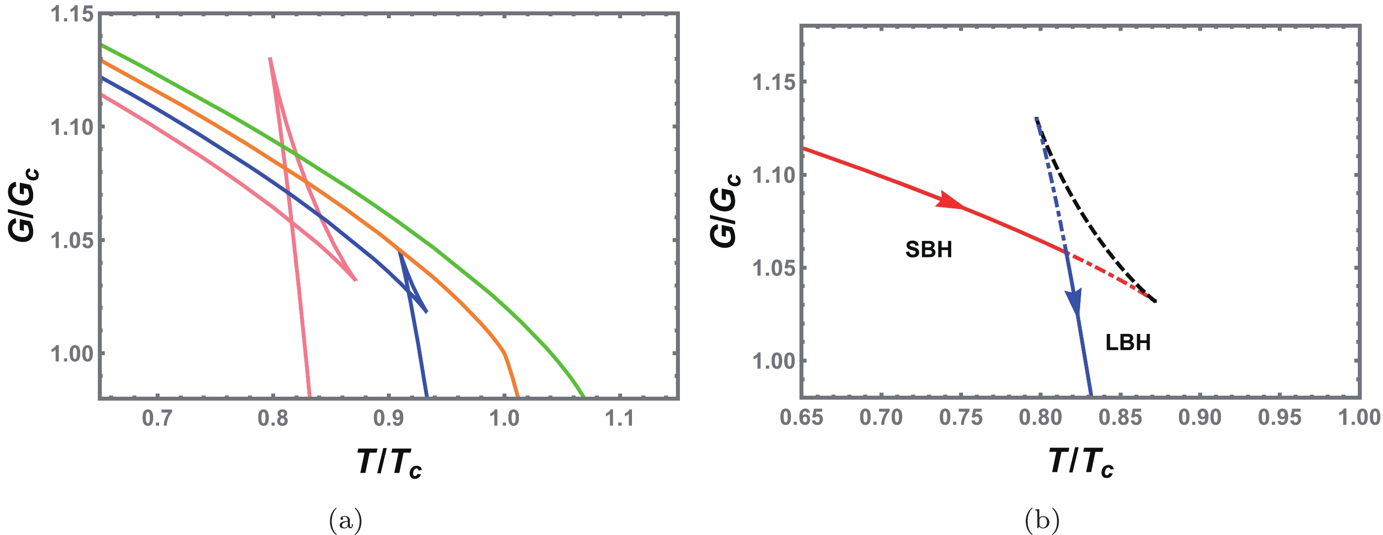

Figure 4.  (color online) (a) Gibbs free energy for ${\tilde{P}}=0.6$ (pink solid line), ${\tilde{P}}=0.8$ (blue solid line), ${\tilde{P}}=1.0$ (orange solid line), and ${\tilde{P}}=1.2$ (green solid line). (b) Small/large black hole phase transition. The small and large black holes are marked with red and blue solid lines, respectively, and are stable; however, the black hole marked with a black dashed line is unstable. Although the red and blue dot dashed lines indicate stable black holes, they are not the minimum value of the Gibbs free energy. Along the direction of the arrow, the volume of the black hole increases. We set $Q=1.0$ and $a=-1.5$.

To clearly show the phase transition, we describe the Gibbs free energy in Fig. 4(b) with $P<P_c$. After a simple calculation, we find that the SBH and LBH branches, indicated by the red and blue solid curves, respectively, have a positive heat capacity, and thus they are thermodynamically stable. In contrast, the branches indicated by dashed curves are unstable or metastable. Considering that a system always prefers a state of low Gibbs free energy, the system will undergo a first-order phase transition from an SBH phase to an LBH phase with an increase in temperature. The phase transition point is precisely located at the intersection of the swallow tail behavior. Thus, it is easy to see that this phase transition is similar to the liquid-gas phase transition of a VdW fluid.

The phase structures of charged EH-AdS black holes are given in Fig. 5, from which we find that they share a similar phase diagram with a VdW fluid. In the P-T diagram, the first-order coexistence curve of the SBH and LBH starts at ${\tilde{T}}=0$ and ends at the critical point, which divides the plane into two regions corresponding to the SBH and LBH phases. Considering that the equation of state is not applicable in the shadow region, we use the spinodal curve marked with the blue dashed curve to distinguish the metastable phase from the coexistence phase of the black hole. The spinodal curve is determined by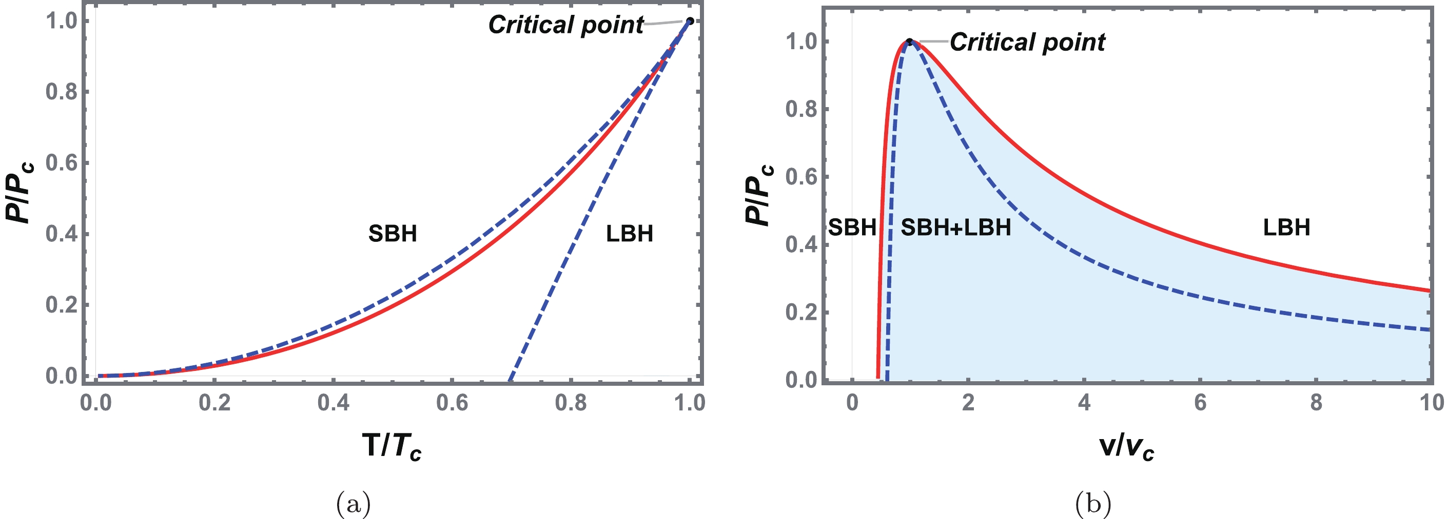

Figure 5.  (color online) Phase diagram for the VdW phase transition type case. (a) First-order coexistence curve (solid red) and spinodal curve (blue dashed line) are shown on the P-T plane. The coexistence curve separates the SBH and LBH phases and ends at a critical point. (b) Phase structure on the P-v plane. The shadow region under the coexistence curve is the coexistence phase of the SBH and LBH. The region between the coexistence curve and spinodal curves is metastable. Here, we take $Q=1.0$ and $a=-1.5$.

Clearly, the spinodal curve meets the coexistence curve at the critical point.

For this case, two critical points can be found. The corresponding phase transition is the reentrant phase transition, including a zero-order and first-order phase transition at a certain region of the temperature or pressure. Here, we study the reentrant phase transition of charged EH-AdS black holes.

As expected, the first-order phase transition can be determined by constructing two equal areas according to Maxwell's equal area law. As shown in Fig. 3(a), the isotherm curves exhibit a nonmonotonic behavior on the P-v plane. Therefore, we can construct two equal areas between two stable black hole branches. However, as pointed out in Ref. [60], the equal areas should be constructed on the P-V plane rather than the P-v plane. Alternatively, Maxwell's equal area law also holds on the ${\tilde{T}}$-${\tilde{S}}$ plane by giving the pressure in either ordinary or reduced parameter space.

where ${\tilde{T}}_0$ denotes the reduced temperature of the phase transition, and ${\tilde{S}}_1$ and ${\tilde{S}}_2$ are the reduced entropy of the corresponding coexistence of the SBH and LBH. Taking ${\tilde{P}}$=0.4 as an example, Maxwell's equal area law is fulfilled on the ${\tilde{T}}$-${\tilde{S}}$ plane in Fig. 6. The black curves denote the SBH and LBH branches. The red curves indicate the two metastable branches, superheated SBH branch, and supercooled LBH branch. The blue curve with a negative slope is an unstable branch and is substituted by a horizontal line according to the equal area law. The area under the isobaric curve from ${\tilde{S}}_{1}$ to ${\tilde{S}}_{2}$ must equal the area enclosed by the rectangle under the isothermal horizontal line to ensure that the areas of the two shadow regions are equal. The two black dots represent the spinodal points, which separate the metastable branches from the unstable branch. Then, the pressure and temperature corresponding to the isothermal horizontal line are simply those of the phase transition point.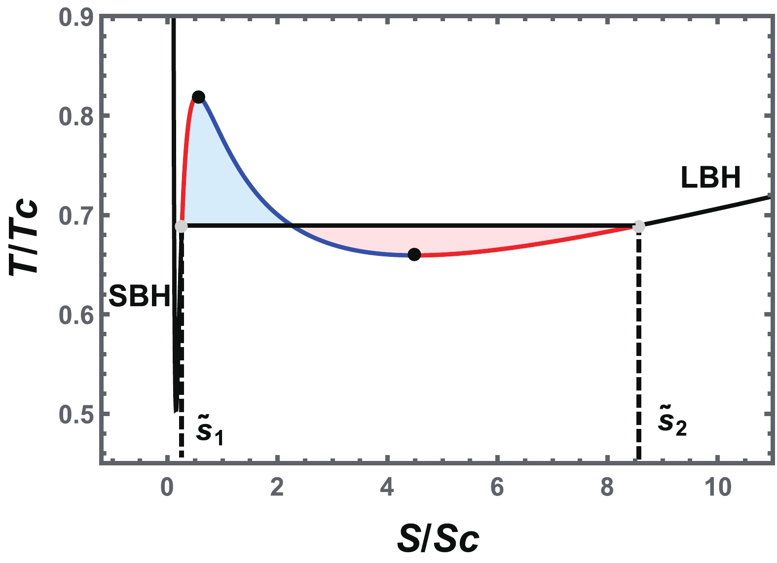

Figure 6.  (color online) Isobaric curve with ${\tilde{P}}=0.4$ and the equal area law on the ${\tilde{T}}$-${\tilde{S}}$ plane, where the two shadow areas above and below the horizontal line are equal. The black curves represent the SBH and LBH branches. The two red curves represent the superheated SBH branch and supercooled LBH branch. The blue curve represents an unstable branch. We set $Q=1.0$ and $a=1.0$.

We depict the Gibbs free energy for these two types of phase transitions in Fig. 7. In Fig. 7(a), the SBH/LBH phase transition is analyzed for the reduced pressure ${\tilde{P}}=0.4$. As the temperature increases, the system jumps directly from the SBH phase (red solid line) to the LBH phase (blue solid line), and the volume of the black hole directly undergoes a sudden change when the temperature is equal to the phase transition temperature. The heat capacity of the black hole branches represented by the black dashed lines is negative, indicating thermodynamic instability. Note that although the black hole branches denoted by the dot dashed lines in the Fig. 7 have a positive heat capacity, they do not have the lowest free energy for a fixed temperature, and thus they are metastable black hole branches. In addition to the SBH/LBH phase transition, another new zero-order phase transition emerges in Fig. 7(b). When the zero-order phase transition occurs, the black hole system jumps from the LBH phase to the SBH phase. In addition to the volume of the black hole undergoing sudden changes, the Gibbs free energy changes drastically. In short, the black hole system first undergoes a zero-order phase transition from the LBH phase to the SBH phase and then returns to the LBH phase via the SBH/LBH phase transition with increasing temperature. A phase transition with this type of pattern is known as a reentrant (large/small/large BH) phase transition.

Figure 7.  (color online) (a) SBH/LBH phase transition with ${\tilde{P}}=0.40$. (b) Reentrant phase transition (large/small/large black hole phase transition) with ${\tilde{P}}=0.19$. The SBH (red solid line) and LBH (blue solid line) are stable, whereas those represented by the black dashed curves are unstable. It is worth noting that the red and blue dot dashed curves correspond to a positive heat capacity. However, they are not the minimum value of the Gibbs free energy and thus are metastable. We set $Q=1.0$ and $a=1.0$.

Phase diagrams of the reentrant phase transition are shown in Fig. 8. Similar to the case of the VdW phase transition type, the coexistence curve (red solid line) divides the parameter space into two regions in Fig. 8(a). Above and below the coexistence curve are the SBH and LBH phases, respectively. The zero-order phase transition line marked with a green solid line connects the first-order coexistence curve and minimum temperature curve. The phase diagram is also shown on the ${\tilde{P}}$-${\tilde{v}}$ plane in Fig. 8(b). The critical point divides the coexistence curve into left and right parts, which correspond to the coexistence SBH and LBH, respectively. The SBH and LBH regions are located on the left and right, respectively.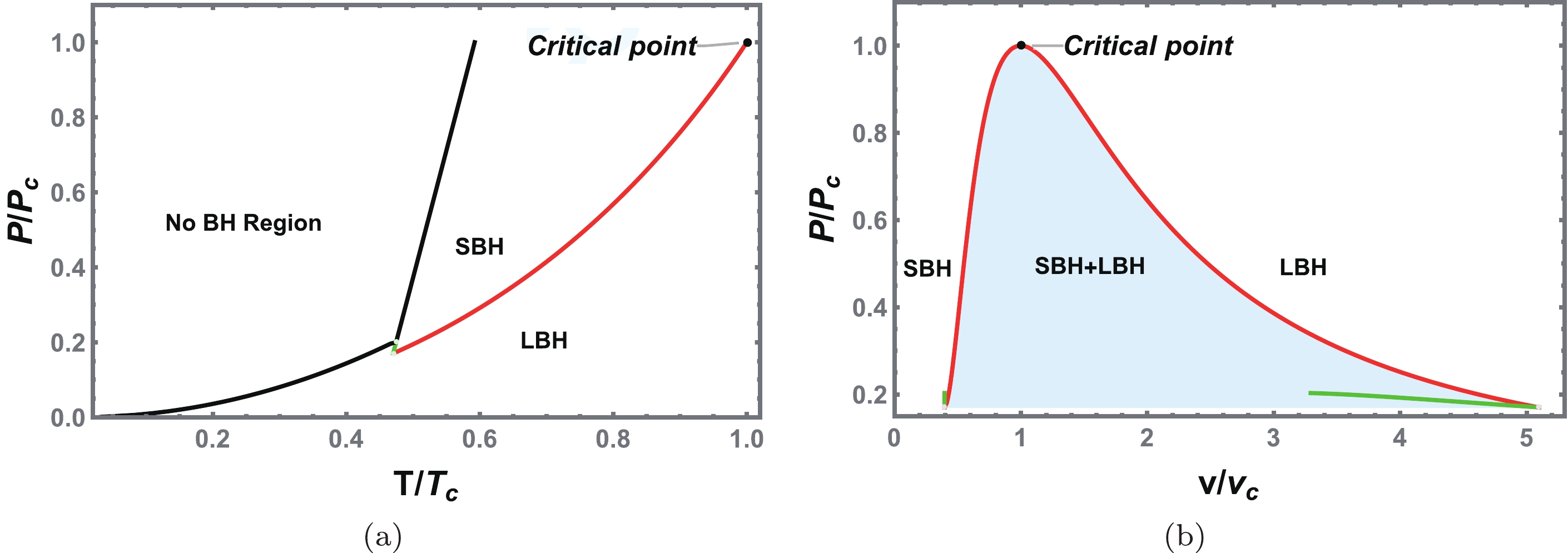

Figure 8.  (color online) Phase diagrams of charged EH-AdS black holes. (a) First-order coexistence curve (solid red) and zero-order phase transition line (solid green) are also shown on the ${\tilde{P}}$-${\tilde{T}}$ plane. The black line separates the no black hole region from the black hole region. The first-order coexistence curve separates the SBH and LBH phases and ends at a critical point. (b) Phase structure in the ${\tilde{P}}$-${\tilde{v}}$ plane. The shadow area under the coexistence curve is the coexistence phase of the SBH and LBH.

In Fig. 9(a) and (b), we plot the difference of the volume $\Delta V=V_{l}-V_{s}$ among first-order phase transitions as a function of temperature and pressure, respectively. It is clear that below the critical point, $\Delta V$ has a finite value, indicating a sudden change during the black hole phase transition. However, when the critical point is reached, $\Delta V$ vanishes, which means that one cannot distinguish between the SBH and LBH anymore. Considering the behavior of $\Delta V$, it can be regarded as an order parameter that characterizes the phase transition.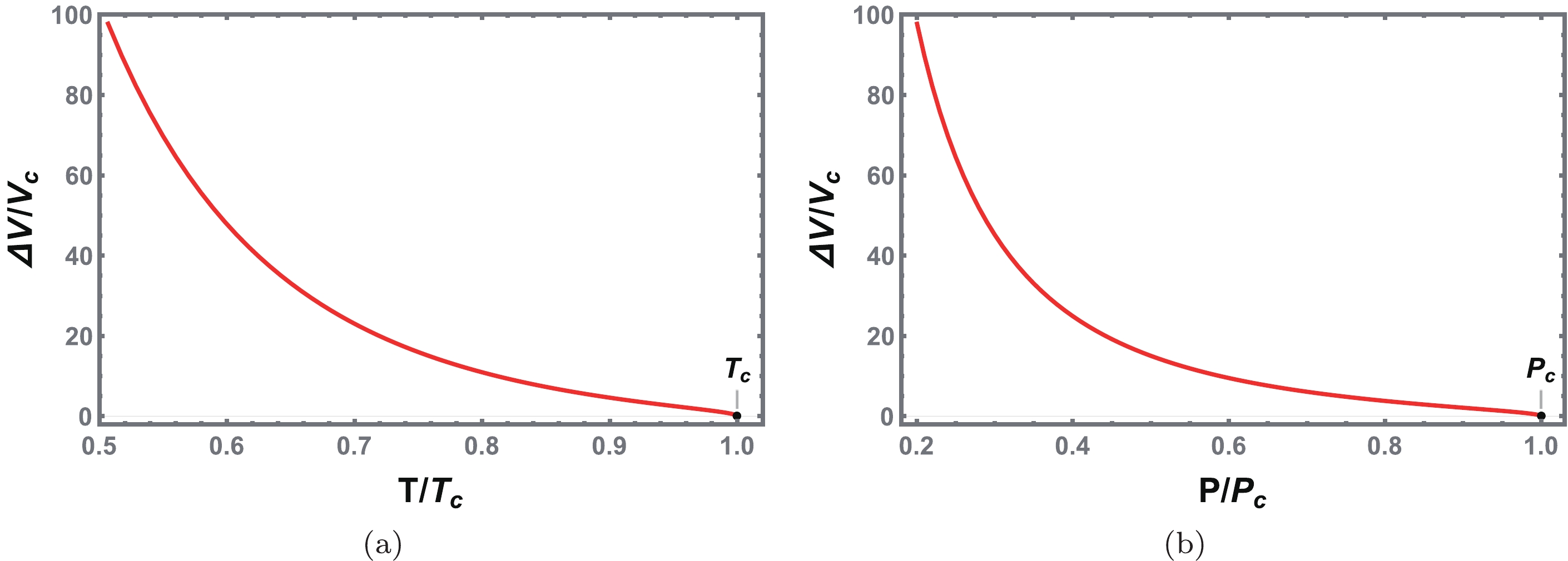

Figure 9.  (color online) Behavior of the change of the thermodynamic volume at the black hole phase transition. (a) $\Delta V$ vs. ${\tilde{T}}$. (b) $\Delta V$ vs. ${\tilde{P}}$. The critical point is at $T_c$ and $P_c$.

Near the critical point, the critical exponent of $\Delta V$ can be calculated (see Ref. [56]). However, in the calculation, the specific volume v is used in constructing the equal area law, which, as we noted, is inappropriate. Here, we make use of the thermodynamic volume V instead and observe whether the result remains unchanged. Using the relationship between thermodynamic volume and specific volume, $V=\dfrac{\pi v^3}{6}$, we get ${\tilde{V}}={\tilde{v}}^{3}$. Then, Eq. (25) can be expressed as

where $\rho_c=\dfrac{P_{c}v_{c}}{T_c}$. Let the first term in the previous equation be the function $h({\tilde{V}})$ so that (29) can be written as

The Taylor expansion in the vicinity of the critical point at ${\tilde{V}}=1$ and ${\tilde{T}}=1$ is written as

From the definition of the critical point, Eq. (31) must meet the following conditions:

Therefore, Eq. (31) can be simplified to

Taking $\omega={\tilde{V}}-1$ and $t={\tilde{T}}-1$, the previous expression becomes

where we define $C=\dfrac{14}{81\,\rho _c}-\dfrac{1}{6} h^{(3)}(1)$. From Maxwell's equal area law, we obtain

where $\omega_l$ and $\omega_s$ are the volumes of the coexistence SBH and LBH, respectively. For an isothermal process, the pressure $P_s$ is equal to $P_l$, i.e., ${\tilde{P}}_s(t,\omega)={\tilde{P}}_l(t,\omega)$, which reads

Combining (35) and (36), we have

The critical exponent β is related to the order parameter $\eta = |t|^{\beta}$, namely, with the change in volume at the phase transition for a given isotherm process,

Therefore, the critical exponent β is

As a result, the choice of specific volume or thermodynamic volume does not change the value of the critical exponent β. However, when applying Maxwell's equal area law, we should choose the thermodynamic volume rather than the specific volume.

In this section, we construct the Ruppeiner geometry of charged EH-AdS black holes, and the microstructure is tested using the curvature scalar.

Here, we first give a brief introduction to Ruppeiner geometry and then calculate the curvature scalar for charged EH-AdS black holes.

Let us consider a thermodynamically isolated system in equilibrium with total entropy S. The system is divided into two subsystems, the small system under consideration and its large environment. Their entropies are denoted by $S_S$ and $S_E$, with $S_{S}\ll S_{E}\sim S$. We suppose that the total entropy of the system is described by two independent thermodynamic variables $x_{0}$ and $x_{1}$. The total entropy of the system can be written as

For a system in equilibrium, the entropy reaches its maximum locally. We perform a Taylor expansion in the neighborhood of this local maximum $(x^{\mu}=x^{\mu}_{0})$

where the zero-order term $S_{0}$ is the local maximum of entropy at $x^{\mu}_{0}$. The entropy of an isolated system in equilibrium is conserved under virtual change. This shows that the first derivative of the entropy vanishes, and thus we get

It is worth noting that $S_{E}$ is a thermodynamic extensive quantity and has the same order of magnitude as the entropy of the entire system. Therefore, its derivative with respect to the intensive quantity $x^{\mu}$ is significantly smaller than the derivative of $S_{S}$, which can be ignored. Therefore, the probability of finding the system in the internals ($x_0$, $x_0+dx_0$) and ($x_1$, $x_1+dx_1$) is

where $k_{\rm B}$ is the Boltzmann constant. With (41), the line element of Ruppeiner geometry that measures the distance between two neighboring fluctuation states can be written as

Because $\Delta l^2$ can measure the distance between two neighboring fluctuation states, the thermodynamic metric $g_{\mu\nu}^{R}$ potentially contains some information about the microstructure of the system.

When we choose the thermodynamic coordinates $x^{\mu}$ to be the temperature T and volume V, the Helmholtz free energy is the thermodynamic potential. The corresponding line element can be written as follows [31]:

where $C_{V}=T(\partial_TS)_{V}$ is the heat capacity at constant volume. Using the convention in literature [32], we can directly calculate the corresponding scalar curvature of the line element.

It should be noted that the sign of scalar curvature characterizes the type of interaction between two microscopic molecules in a given system [61], i.e., $R>0$ and $R<0$ represent a dominant repulsive interaction and attractive interaction, respectively. For VdW fluids, the study shows that it has a negative scalar curvature, indicating a dominant attractive interaction between these underlying molecules. In addition, when $R=0$, the interactions of repulsion and attraction reach equilibrium [62].

For charged EH-AdS black holes, the heat capacity at constant volume vanishes. Adopting the treatment in Ref. [38], the new normalized scalar curvature $R_N$ is

Using the equation of state (23), the normalized scalar curvature of a charged EH-AdS black hole reads

where

We plot the scalar curvature $R_N$ as a function of ${\tilde{V}}$and ${\tilde{T}}$ in Fig. 10 for the SBH/LBH phase transition and reentrant phase transition. It can be observed that the surface of the normalized scalar curvature is concave where the scalar curvature diverges. Moreover, compared with the VdW type phase transition, a new divergence occurs in the reentrant phase transition when the reduced volume ${\tilde{V}}$ is close to zero.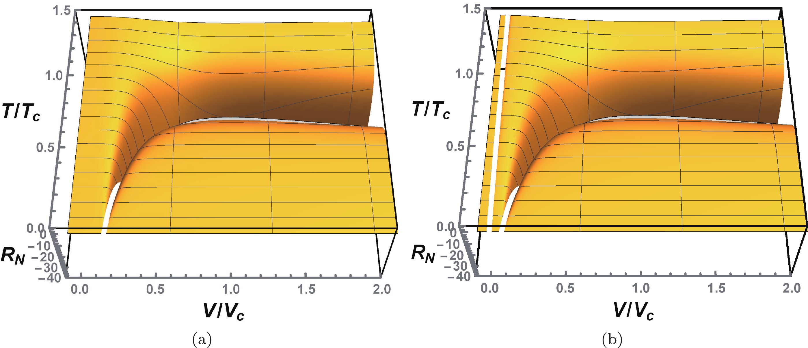

Figure 10.  (color online) Behavior of the normalized scalar curvature $R_N$ as a function of ${\tilde{V}}$ and ${\tilde{T}}$ for charged EH-AdS black holes. (a) VdW phase transition type case with $Q=1.0$ and $a=-1.5$. (b) Reentrant phase transition case with $Q=1.0$ and $a=1.0$.

As shown above, there is an SBH/LBH phase transition of the VdW-type for this case.

To reveal the details, we take $Q=1.0$ and $a=-1.5$ and illustrate the normalized scalar curvature $R_{N}$ as a function of ${\tilde{V}}$ for fixed reduce temperature ${\tilde{T}}$= 0.4, 0.8, 1.0, and 1.2 in Fig. 11. For $T<T_c$, there are two divergent points of the normalized scalar curvature $R_N$. These two points get closer as the temperature increases. At the critical temperature, these two points merge. When $T>T_c$, the normalized scalar curvature $R_N$ does not diverge while maintaining finite values. In most of the parameter space, $R_N$ is negative, whereas in a small region of ${\tilde{V}}$ for ${\tilde{T}}$= 0.4, shown in the inset of Fig. 11(a), $R_N$ is positive. This phenomenon indicates that the dominant repulsive interaction may exist in some parameter regions.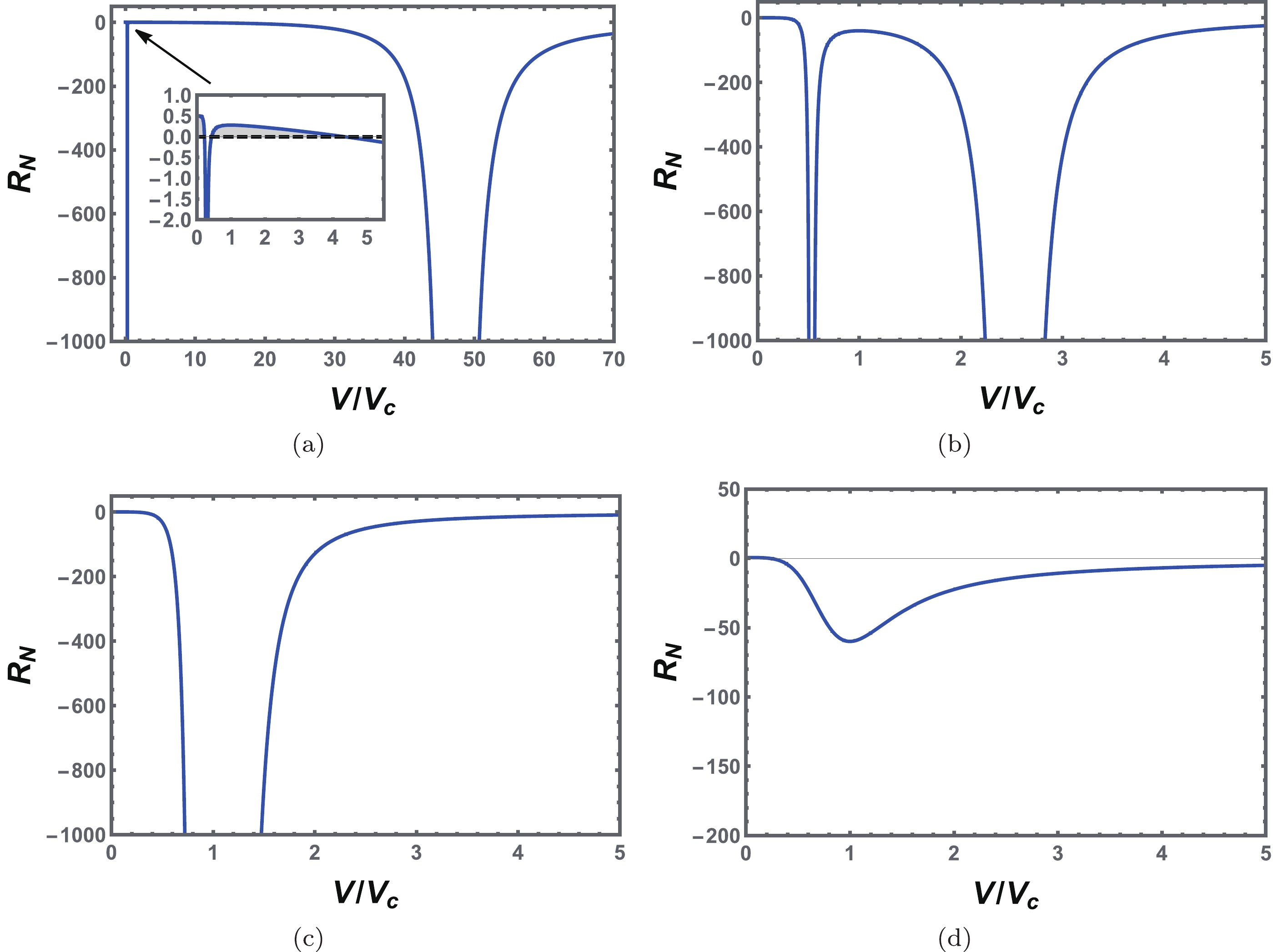

Figure 11.  (color online) Behavior of the normalized scalar curvature $R_N$ with the reduced volume ${\tilde{V}}$ at a constant temperature. (a) ${\tilde{T}}=0.4$. (b) ${\tilde{T}}=0.8$. (c) ${\tilde{T}}=1.0$. (d) ${\tilde{T}}=1.2$. The inset shows the enlarged portion near the origin, and $R_N$ has positive values, which is depicted by shadow regions. We set $Q=1.0$ and $a=-1.5$.

From the analysis of the normalized scalar curvature $R_{N}$, it is clear that the divergent point of $R_{N}$ satisfies the spinodal point condition $(\partial_{V} P)_{T}=0$, which gives

After a simple calculation, the specific expression of the sign changing curve corresponding to $R_{N}=0$ reads

which indicates that the temperature of the sign changing curve is half of the temperature of the spinodal curve [31, 38].

In Fig. 12(a), the sign changing curve (black dot dashed line), spinodal curve (blue dashed line), and coexistence curve (red solid line) are displayed. The shadow regions I and II have a positive scalar curvature, whereas the other regions have a negative scalar curvature. Because the equation of state of the charged EH-AdS black hole in region II is no longer valid, this region must be excluded. However, in region I, the SBH with high temperature still exhibits the dominant repulsive interaction. This is similar to the situation of charged RN-AdS black holes, but different from that of neutral black holes in Gauss-Bonnet gravity [39, 63]. The negative parameter a increases the effective black hole charge, which strengthens the repulsive interaction between black hole micromolecules of small size. However, a method of establishing a precise microscopic interpretation between the effect of QED and Ruppeiner geometry remains to be further explored.

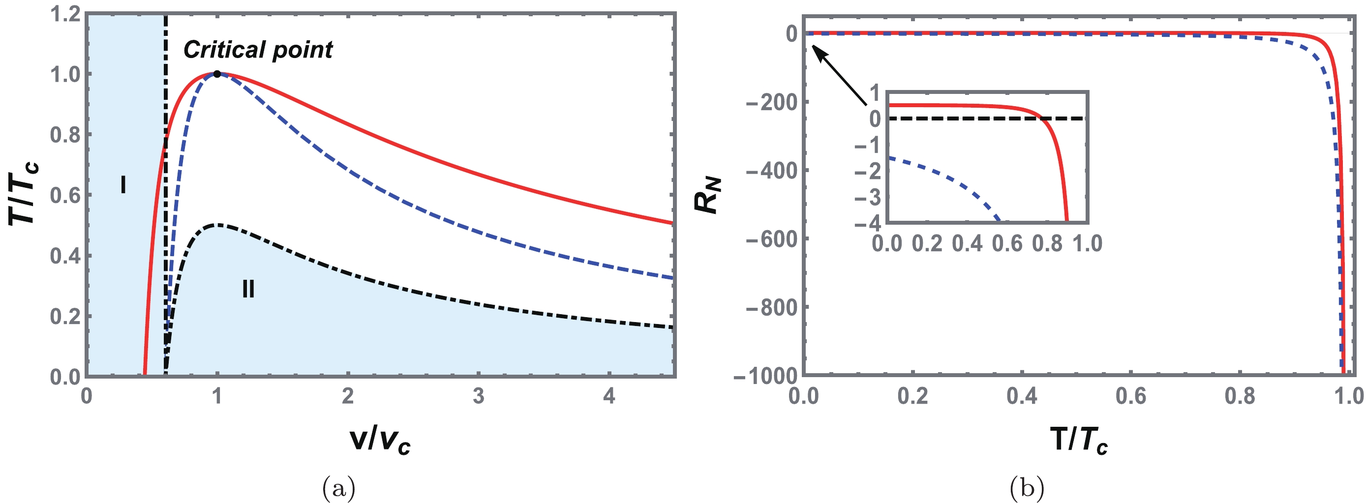
Figure 12.  (color online) (a) Sign changing curve of $R_N$ (black dot dashed line), spinodal curve (blue dashed line), and coexistence curve (red solid line) for the VdW type phase transition case. The shadow regions marked with I and II correspond to positive $R_N$, otherwise $R_N$ is negative. (b) Behavior of the normalized Ruppeiner curvature scalar $R_N$ along the coexistence curve. The red solid and blue dashed lines correspond to the SBH and LBH, respectively. The change in the nature of the SBH interaction is shown in the inset. We set $Q=1.0$ and $a=-1.5$.

We show the behavior of $R_N$ along the coexistence SBH and LBH in Fig. 12(b). It is clear that both tend toward negative infinity at the critical temperature, indicating the existence of the critical exponent. Moreover, we find that $R_N$ of the coexistence SBH is always above that of the LBH. At low temperature, the coexistence SBH has a positive value, which is consistent with Fig. 12(a).

Because the critical exponent can provide us with some universal properties, we now calculate it for the scalar curvature at the critical point. Here, it is natural to assume that the normalized scalar curvature $R_N$ near the critical point has the following form [64]:

or equivalently,

By calculating $R_N$ near the critical point, we obtain the following fitting results:

The numerical results (small red dots) and fitting results (blue solid lines) are shown in Fig. 13. The numerical and fitting results are highly consistent with each other. The slopes obtained by fitting the coexistence curves of the SBH and LBH are $\alpha_{\rm SBH}$=2.0365 and $\alpha_{\rm LBH}$=1.9636, respectively. Considering the error on the numerical calculation, the critical exponent is $\alpha=2$, which is the same as that of a VdW fluid.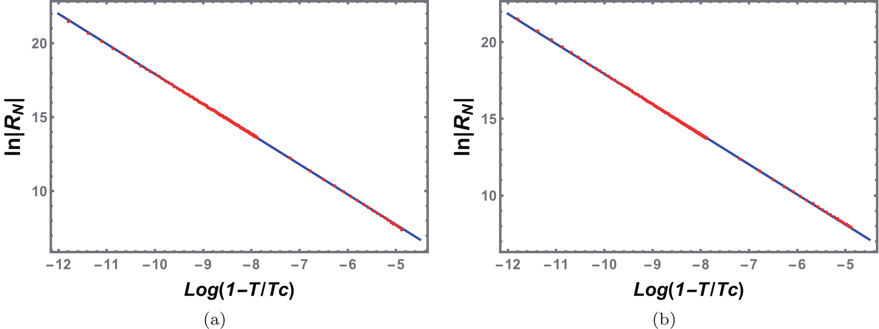

Figure 13.  (color online) Fitting curves of $\ln |R_N|$ vs. $\ln (1-{\tilde{T}})$ near the critical point. The red dots are numerical data, and the blue solid lines are obtained from the fitting formulas. (a) Coexistence SBH branch. (b) Coexistence LBH branch.

Moreover, using the intercept β obtained from the fitting results, we obtain a dimensionless constant

This has the same value for charged AdS black holes and VdW fluids and is also consistent with the result obtained in Ref. [56] by expanding the equation of state near the critical point at the first leading term.

We explore the underlying microstructure of the black hole that results in a reentrant phase transition with Q = 1 and a = 1 using a similar method. The behavior of $R_N$ against the reduced thermodynamic volume ${\tilde{V}}$ for a fixed temperature is shown in Fig. 14. Compared with the VdW phase transition, the scalar curvature of the reentrant phase transition has an additional divergent point near the origin. This is because when $T<T_c$, there are three extremal points on each isothermal curve (see Fig. 3(b)). As the temperature increases, the evolution behavior of other two divergent points is very similar to the case of the VdW-like phase transition. Furthermore, when the temperature is higher than its critical value, the additional divergent point still exists. However, when the reduced volume is close to the origin, positive scalar curvature is observed as expected.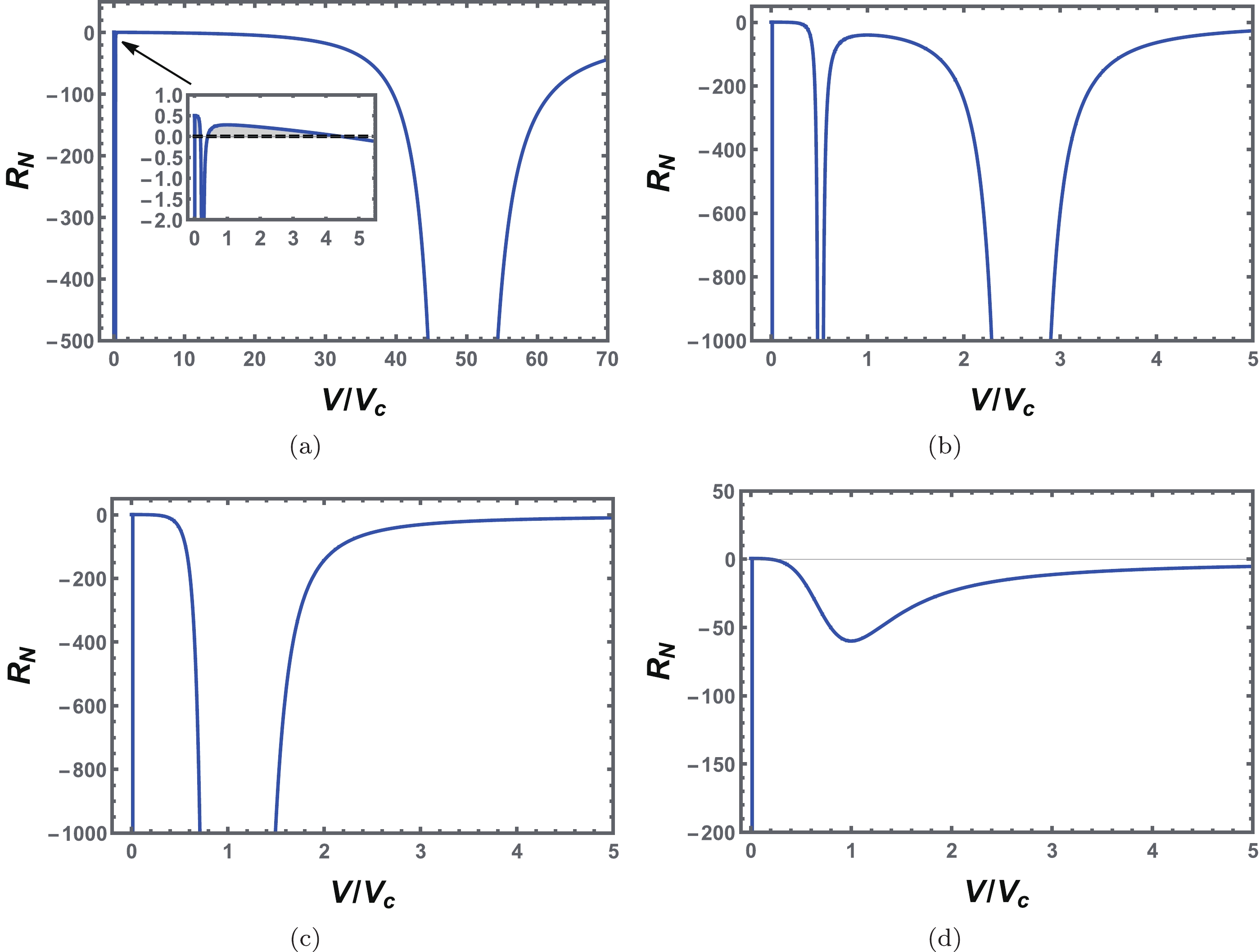

Figure 14.  (color online) Behavior of the normalized scalar curvature $R_N$ with the reduced volume ${\tilde{V}}$ at a constant temperature for the reentrant phase transition case. (a) ${\tilde{T}}=0.4$. (b) ${\tilde{T}}=0.8$. (c) ${\tilde{T}}=1.0$. (d) ${\tilde{T}}=1.2$. The inset shows the enlarged portion near the origin, and $R_N$ has positive values. We set $Q=1.0$ and $a=1.0$.

The first-order coexistence curve, zero-order phase transition curve, spinodal curve, and sign changing curve are depicted in Fig. 15(a). In the shadow regions I, II, and III, the scalar curvature takes positive values. Compared with the VdW-like phase transition, the number of shadow regions is three instead of two. The leftmost part of the coexistence curve of the SBH ends at the spinodal curve and indicates a divergence. However, one should note that the black hole does not exist in region I.

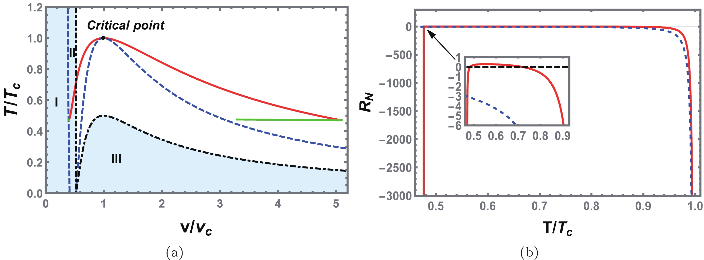
Figure 15.  (color online) (a) Sign changing curve of $R_N$ (black dot dashed line), spinodal curve (blue dashed line), first-order coexistence curve (red solid line), and zero-order phase transition line (green solid line) for the reentrant phase transition case. The shadow regions marked with I, II, and III correspond to positive $R_N$, otherwise $R_N$ is negative. (b) Behavior of the normalized scalar curvature $R_N$ along the coexistence curve. The red (solid) and blue (dashed) lines correspond to the SBH and LBH, respectively. The change in the sign of $R_N$ of the SBH is shown in the inset.

We also plot the normalized scalar curvature $R_{N}$ along the coexistence SBH and LBH curves as a function of temperature in Fig. 15(b). Along the coexistence curve, $R_N$ negatively diverges at the critical point for both the SBH and LBH. However, in contrast with the previous VdW-like phase transition, the scalar curvature of the SBH gains a new divergence when the reduced temperature is approximately 0.48. For the coexistence LBH, there is no such phenomenon. The reason for this new divergence is that the leftmost part of the coexistence SBH curve is located on the spinodal curve, but that of the LBH is not.

Near the critical point, the fitting results for the coexistence SBH and LBH are given by

The numerical and fitting results are shown in Fig. 16 and are highly consistent with each other. The fitting coefficients of the LBH and SBH are $\alpha_{\rm LBH}$ =1.9536 and $\alpha_{\rm SBH}$ =2.0426, respectively. Considering the error on the calculation, we obtain the critical exponent $\alpha=2$. The dimensionless constant is

Figure 16.  (color online) Fitting curves of $\ln R_N$ vs. $\ln (1-{\tilde{T}})$ near the critical point for the reentrant phase transition. The red dots are numerical data, and the blue solid lines are obtained from the fitting formulas. (a) Coexistence SBH branch. (b) Coexistence LBH branch.

which is the same as that of the VdW-like phase transition.

In this study, we investigate the phase transition and Ruppeiner geometry in different ranges of the QED parameter in the extended phase space. For $a<0$ and $0 \leq a \leq \dfrac{32 Q^2}{7}$, we observe the SBH/LBH phase transition and reentrant phase transition, respectively, whereas for $\dfrac{32 Q^2}{7} < a$, there is no first-order phase transition. In these different ranges, we explore the black hole microstructure, and different potential interactions are uncovered for charged EH-AdS black holes.

First, we investigate the thermodynamic properties of the black hole phase transition. Treating the cosmological constant and QED parameter as two new variables, we find that the first law of black hole thermodynamics and the Smarr formula hold. We also confirm that they are consistent with each other in the extended phase space. Furthermore, using the Hawking temperature, we obtain the equation of state and hence the critical point. It is shown that for $a<0$, $0 \leq a \leq \dfrac{32 Q^2}{7}$, and $\dfrac{32 Q^2}{7} < a$, one, two, and zero critical points can be observed. Based on this, we study the phase transition in these parameter ranges.

For a negative QED parameter a, we observe a characteristic swallow tail behavior of the Gibbs free energy below the critical point, which indicates that there is a typical first-order black hole phase transition. Phase diagrams are also explicitly shown. When $0 \leq a \leq \dfrac{32 Q^2}{7}$, two critical points are observed, which indicates a rich phase transition beyond the SBH/LBH phase transition. For certain values of temperature or pressure, four black hole branches are found, two of which are unstable, while the other two are stable. From the behavior of the Gibbs free energy, the two stable branches form a reentrant phase transition. We then show the phase diagrams, which differ from those of the SBH/LBH phase transition of the VdW type. When the QED parameter has a large value such that $\dfrac{32 Q^2}{7} < a$, only one black hole branch is stable, and thus no black hole phase transition exists.

Next, we study the microstructure using Ruppeiner geometry. Taking (T, V) as two fluctuation coordinates in thermodynamic phase space, we construct the Ruppeiner geometry and calculate the corresponding normalized scalar curvature of charged EH-AdS black holes. The scalar curvature behaves differently for the SBH/LBH phase transition and reentrant phase transition, which may be due to their different phase structures. For the SBH/LBH phase transition, the normalized scalar curvature has at most two divergent points for each isothermal curve, whereas for the reentrant phase transition, an additional divergent point near a small volume is observed.

Using the empirical observation of Ruppeiner geometry, we find that, with a negative QED parameter, the repulsive interaction dominates in the microstructure of the SBH with high temperature, whereas the attractive interaction dominates for other black holes. This result is similar to that of a charged AdS black hole without the QED parameter. For a charged EH-AdS black hole with a small QED parameter, another region of positive scalar curvature emerges, which is below, but not surrounded by, the coexistence curve of the first-order phase transition. As a result, in contrast with the SBH/LBH phase transition, the equation of state is applicable for this case. Therefore, low temperature black holes may be dominated by the repulsive interaction.

Furthermore, the behavior of the scalar curvature along the first-order coexistence curve of the SBH and LBH is carefully analyzed. In the case of a = –1.5 and Q = 1, the scalar curvature for both the coexistence SBH and LBH decreases and tends to negative infinity at the critical temperature. However, for a = 1 and Q = 1, the reentrant phase transition is present. Except for the divergent point near the critical point, the scalar curvature of the coexistence SBH also diverges near ${\tilde{T}}$=0.48, which is mainly because the starting point of the coexistence SBH curve is on the spinodal curve. This is also a novel feature of the reentrant phase transition.

In particular, through numerical calculation, we observe a critical exponent of 2 and a dimensionless constant of $-{1}/{8}$ near the critical point for the scalar curvature. These results are the same as those of other black holes and VdW fluids, suggesting a solution of mean-field theory.

Our study is a complete investigation of the phase transition and microstructure of charged EH-AdS black holes. The effects of the QED parameter on black hole thermodynamics are examined in detail. Using the geometric method, interactions inside the microstructure are uncovered. These results help us understand the nature of black holes with a QED correction from the viewpoint of thermodynamics.