


 Abstract
 HTML
HTML Reference
 Related
 PDF
PDF


-
Heavy hadron decays provide an ideal platform for precision tests of the unitarity of the Cabbibo-Kobayashi-Maskawa (CKM) matrix to investigate CP violation in the standard model (SM) and search for new physics (NP) signals beyond the SM. In the past few years, unexpected anomalies have been presented at the observables
$ R_D,R_{D^\ast} $ of semileptonic B decays induced by the$ b\to c\ell\nu $ transition, where SM predictions deviate from data at the$ (2 \sim 3)\sigma $ level (see, for example, [1–10]), and QED corrections also cannot lead to large corrections to$ R_D,R_{D^\ast} $ [11, 12]. These anomalies might relate to the violation of lepton flavor universality (LFU), which hints at the existence of NP signals. Therefore, many NP models have been proposed to explain such tensions, such as$ W' $ models, leptoquark models, and models with charged Higgs (see [13, 14] and the references therein). Other than$ B\to D(D^\ast)\ell\nu $ decays, the weak decays of heavy baryons, such as$ \Lambda_b\to \Lambda_c\ell \nu $ , are also mediated by the$ b\to cl\nu $ transition, which may provide further hints to make this "anomaly" more transparent (for a review, see [15]).The fundamental ingredients of semileptonic
$ \Lambda_b\to \Lambda_c\ell \nu $ decays are the$ \Lambda_b\to \Lambda_c $ transition form factors. For heavy-to-heavy transition processes, the heavy quark effective theory (HQET) [16–18] provides a natural theoretical framework to analyze form factor relations and estimate power corrections. In the heavy quark limit, only one single independent form factor, namely, the Isgur-Wise function$ \xi(v\cdot v') $ [19], appears in the$ \Lambda_b\to \Lambda_c $ transition, and$ \xi(v\cdot v') $ satisfies the normalization condition$ \xi(1)=1 $ . Heavy quark symmetry is effective in the small recoil region, where the$ \Lambda_c $ baryon is almost static, and lattice QCD simulation based on first principles is also highly suitable for application in this region. Predictions of the$ \Lambda_b \to \Lambda_c $ form factors with lattice QCD are given in [20]. One must employ phenomenological models to extrapolate the results across the entire momentum region. To reduce model dependence, it is useful to calculate the form factor in the large recoil region directly. There have been several studies using various approaches, such as quark models [21–27], the perturbative QCD (PQCD) approach [28], and a combination of HQET and PQCD [29].The QCD sum rules method is a popular approach to evaluate hadronic parameters according to the quark-hadron duality ansatz. Three-point QCD sum rules have been widely used in the study of transition form factors. The
$ \Lambda_b\to \Lambda_c $ and$ \Xi_b\to \Xi_c $ transition form factors were studied using three-point QCD sum rules in [30–36]. For heavy-to-light form factors, light-cone sum rules (LCSR) are more appropriate because the light-cone dominance of correlation functions has been proven in the large recoil region [37–39]. In$ \Lambda_b \to \Lambda_c $ decays, the final state$ \Lambda_c $ moves rapidly in the large recoil region; thus, light-cone OPE is applicable. In this paper, we start from the correlation function defined by the matrix element with the time-ordered product of the$ b\to c $ transition weak current and the interpolation current of the$ \Lambda_c $ baryon sandwiched between the vacuum and the$ \Lambda_b $ state, as proposed in [40–42]. These heavy-hadron LCSR have been employed to study the various decay channels of B-mesons [43–48] and the decays of the$ \Lambda_b $ baryon [49–52]. Similar to$ B \to D $ decays, LCSR with$ \Lambda_b $ distrubution amplitudes (DAs) are valid approximately in the momentum region$ 0\leq q^2\leq 8 $ GeV2. In [53], the Isgur-Wise function in$ \Lambda_b \to \Lambda_c $ transitions was studied using LCSR with$ \Lambda_b $ -DAs. A recent study on these form factors is presented in [54]. In this paper, we make the following improvements:● Most previous studies concentrated on the Isgur-Wise function, which arises in the heavy quark limit. For physical form factors, especially in the large recoil region of the final state
$ \Lambda_c $ , large power corrections from the expansion of$ 1/m_c $ need to be made. In the present study, we do not perform heavy quark expansion on the charm quark field; instead, we take advantage of the charm quark field in full QCD to construct the intepolation current of the$ \Lambda_c $ baryon in the correlation function.● We employ the full set of three-particle DAs of
$ \Lambda_b $ up to twist-5, which is accomplished in [55], where the projector of the DAs in the momentum space is also presented. Because models of the DAs of the$ \Lambda_b $ -baryon are not well established, we adopt three different models, that is, the QCDSR model, which is constructed based on QCD sum rules, exponential model, and free parton model, which is proposed by mimicking the B-meson DAs for a comparison.● In previous studies, the heavy b quark was expanded in HQET, and only the leading power contribution was considered. To improve the accuracy of our predictions, we include
$ 1/m_b $ corrections to the heavy quark field in HQET in this study.● When evaluating the correlation function in the hadronic representation, we insert not only the
$ \Lambda_c $ meson but also the parity odd counter particle of the$ \Lambda_c $ baryon, which can help us extract the form factor without ambiguity by solving the obtained sum rule equation.This paper is organized as follows: In the next section, we calculate an analytic expression of the
$ \Lambda_b \to \Lambda_c $ form factors with$ \Lambda_b $ -LCSR at the tree level and investigate the power suppressed contribution from the power suppressed heavy quark field. In Section III, we present the numerical results of the form factors and the experimental observations. We summarize this study in Section IV. -
The heavy-to-light
$ \Lambda_b \to \Lambda_c $ form factors induced by a$ V-A $ current are defined as$ \begin{aligned}[b]& \langle \Lambda_{c}(p',s')|\bar{c}\gamma_{\mu}(1-\gamma_{5})b|\Lambda_{b}(P,s)\rangle \\ =&\bar{u}(p',s')\left[f_{1}(q^{2})\gamma_{\mu}+f_{2}(q^{2})v_{\mu}+f_{3}(q^{2}){v'_{\mu}} \right]u(P,s) \\ &-\bar{u}(p',s')\left[g_{1}(q^{2})\gamma_{\mu}+g_{2}(q^{2})v_{\mu}+g_{3}(q^{2}){v'_{\mu}} \right]\gamma_{5}u(P,s), \end{aligned} $

(1) where
$ P, s $ and$ p',s' $ are the momenta and spins of the baryon in the initial and final state, respectively, and$ v'=p'/m_{\Lambda_c} $ ,$ q=P-p' $ denotes the momentum transfer. In the heavy quark limit, that is,$ m_b,m_c \to \infty $ , the form factors$ f_1 $ and$ g_1 $ are reduced to one unique Isgur-Wise function$ \zeta(w) $ , where$ w=v\cdot v' $ , and$ f_2=f_3=g_2=g_3=0 $ . At the zero recoil limit$ v\cdot v'=1 $ , we have the normalization condition$ \zeta(1)=1 $ . Because we do not perform heavy quark expansion with respect to the charm quark in this study and only take the heavy quark limit of the bottom quark, there are two independent form factors in the$ \Lambda_b \to \Lambda_c $ transition. The most general form of the matrix element$ \langle \Lambda_c(p')|\bar c\Gamma b_v|\Lambda_b(v)\rangle $ consistent with heavy quark spin symmetry reads$ \langle \Lambda_c(p')|\bar c\Gamma b_v|\Lambda_b(v)\rangle= \bar u(p')(\zeta_1+\zeta_2 \not v)\Gamma u(v), $

(2) where
$ \zeta_1(q^2) $ and$ \zeta_2(q^2) $ are the two independent form factors. The form factors$ f_i(q^2) $ and$ g_i(q^2) $ can be expressed as$ \begin{aligned}[b]& f_1=\zeta_1-\zeta_2,\,\, g_1=\zeta_1+\zeta_2,\\& f_2=g_2=2\zeta_2, \,\,f_3=g_3=0. \end{aligned} $

(3) In the next section, we estimate the power suppressed contributions from heavy quark expansion. The above relation still holds after including this power correction because we neglect the contribution from the four-particle LCDAs of
$ \Lambda_b $ . In literature, there is another widely used parameterization of the$ \Lambda_b \to \Lambda_c $ form factors, that is,$\begin{aligned}[b]\langle \Lambda_{c}(p',s')|\bar{c}\gamma_{\mu}(1-\gamma_{5})b|{\Lambda_b}(P,s)\rangle =&\bar{u}(p',s')\left[F_{1}(q^{2})\gamma_{\mu}+F_{2}(q^2){\rm i} \sigma_{\mu\nu}\frac{q^{\nu}}{m_{\Lambda_b}}+F_{3}(q^{2})\frac{q_{\mu}}{m_{\Lambda_b}} \right]u(P,s) \\ &-\bar{u}(p',s')\left[G_{1}(q^{2})\gamma_{\mu}+G_{2}(q^2){\rm i}\sigma_{\mu\nu}\frac{q^{\nu}}{m_{\Lambda_b}}+G_{3}(q^{2})\frac{q_{\mu}}{m_{\Lambda_b}} \right]\gamma_{5}u(P,s), \end{aligned}$

(4) and these form factors are related to
$ f_i,g_i $ defined in Eq. (1) by$ \begin{aligned}[b]& f_1=F_1-\frac{m_{\Lambda_b}+m_{\Lambda_c}}{m_{\Lambda_b}}F_2, \,\, f_2=F_2+F_3, \, \, f_3=\frac{m_{\Lambda_c}}{m_{\Lambda_b}}(F_2-F_3), \\& g_1=G_1+\frac{m_{\Lambda_b}-m_{\Lambda_c}}{m_{\Lambda_b}}G_2,\,\, g_2=G_2+G_3, \, \, g_3=\frac{m_{\Lambda_c}}{m_{\Lambda_b}}(G_2-G_3), \end{aligned}$

(5) After taking the heavy bottom quark limit, the form factors
$ F_i $ and$ G_i $ can be expressed in terms of$ f_i $ as follows:$ \begin{aligned}[b] F_1=&f_1+{1\over 2}(1+r_\Lambda)f_2,\quad F_2={1\over 2}f_2, \\ G_1=& F_1,\quad G_2=G_3=F_3=F_2, \end{aligned} $

(6) where
$ r_{\Lambda}=m_{\Lambda_c}/m_{\Lambda_b} $ . -
Following the standard strategy, we start with the construction of the correlation function
$ \Pi^a_{\mu, i}(q, p')= {\rm i} \int {\rm d}^4 x \, {\rm e}^{{\rm i} p' \cdot x} \, \langle 0 |T \{\eta^{a}(x), j_{\mu, i}(0) \}| \Lambda_b(v) \rangle \,, $

(7) where the local current
$ \eta^a $ interpolates$ \Lambda_c $ , and$ j_{\mu, i} $ represents the weak transition current$ \bar c \, \Gamma_{\mu, i} \, b $ , with the index "i" indicating a certain Lorenz structure, that is,$ j_{\mu, V} =\bar c \, \gamma_{\mu} \, b\,, \qquad \qquad j_{\mu, A}=\bar c \, \gamma_{\mu}\, \gamma_5 \, b\,. $

(8) For the interpolation current of the
$ \Lambda_c $ baryon, as discussed in [37], there are three independent choices.$ \begin{aligned}[b] \eta^{P}=& \epsilon^{ijk}(u^iC\gamma_5d^j)c^k \\ \eta^{A}=&\epsilon^{ijk}(u^iC\gamma_5\gamma_\mu d^j)\gamma^\mu c^k \\ \eta^{S}=&\epsilon^{ijk}(u^iCd^j)\gamma_5c^k \end{aligned} $

(9) where
$ i, j, $ and k are the color indices, and C is the charge conjugation operator. The correlation function will vanish if the S-type current is employed; thus, we only adopt the P-type and A-type operators in our study. The coupling of$ \Lambda_c $ , as well as its party odd partner, with the interpolating current$ \eta^a $ (the decay constant) is defined as$ \begin{aligned}[b]\\[-5pt] \langle 0|\eta^a|\Lambda_c\rangle =& m_{\Lambda_c}\lambda^a_{\Lambda_c}u(p') \\ \langle 0|\eta^a|\Lambda^\ast_c\rangle =& m_{\Lambda^\ast_c}\lambda^a_{\Lambda^\ast_c}\gamma_5u(p') \end{aligned} $

(10) At the hadronic level, the correlation function can be expressed in terms of the matrix elements of the currents sandwiched by the hadronic states
$ \begin{aligned}[b] &\Pi^a_{ \mu,i}\\=& \frac{1}{m_{\Lambda_c}-p^{\prime 2}}\sum\limits_{s'}\langle 0\left|\eta^{a}\right| \Lambda_c\left(p^{\prime},s'\right)\rangle\langle \Lambda_c\left(p^{\prime},s'\right)\left| j_{\mu, i}(0)\right| \Lambda_b(v,s)\rangle \\ & + \frac{1}{m_{\Lambda^\ast_c}^{2}-p^{\prime 2}} \sum\limits_{s'}\langle 0|\eta^a| \Lambda^\ast_c(p^{\prime},s')\rangle \langle \Lambda^\ast_c(p^{\prime},s')|j_{\mu,i}(0)| \Lambda_b(v,s)\rangle\\ &+ {1\over \pi} \int_{s_0}^\infty {{\rm d}s\over s-p'^2-{\rm i} 0}\left[\rho_{1i}^h(s)\gamma_\mu+\rho_{2i}^h(s)v_\mu+\rho_{3i}^h(s)v'_\mu\right ]\Lambda_b(v), \end{aligned}$

(11) where
$ \rho^h_{ai}(s) $ denotes the hadronic spectral densities of all excited and continuum states with the quantum numbers of$ \Lambda_c $ and$ \Lambda_c^\ast $ . It is then a straightforward task to write the hadronic representations of the correlation functions defined with various weak currents. For the vector current, we have the following expression.$ \begin{aligned}[b] \Pi^a_{\mu, V}(p', q) =& \frac{m_{\Lambda_c}\lambda^a_{\Lambda_c} } {m_{\Lambda_c}^2 -p^{\prime 2} } \left(\not p^{\prime}+m_{\Lambda_c}\right)\Big[\gamma_{\mu}f_{1}(q^{2})\\&+v_{\mu}f_{2}(q^{2}) +{v'_{\mu}}f_{3}(q^{2}) \Big] u\left(v, s\right) \\& +\frac{m_{\Lambda_c^\ast}\lambda^a_{\Lambda_c^\ast} } {m_{\Lambda_c^\ast}^2 -p^{\prime 2} } \left(-\not p^{\prime}+m_{\Lambda_c^\ast}\right)\\&\times\left[\gamma_{\mu}\tilde f_{1}(q^{2})+v_{\mu}\tilde f_{2}(q^{2}) +{v'_{\mu}}\tilde f_{3}(q^{2})\right] u\left(v, s\right)+... \end{aligned} $

(12) For
$ \Pi^a_{\mu, A}(p', q) $ , only the replacement$ f_i\to g_i, \tilde f_i \to \tilde g_i $ is required. Through the analysis of the Lorentz structures, the correlation function can be parameterized as$\begin{aligned}[b] \Pi^a_{ \mu, V}(p', q) =& \Big[\Pi^a_{1+}\gamma_\mu+\Pi^a_{1-}\not p^{\prime}\gamma_\mu+\Pi^a_{2+}v_\mu +\Pi^a_{2-} v_\mu\not p^{\prime}\\&+\Pi^a_{3+}v'_\mu +\Pi^a_{3-}\not p^{\prime}v'_\mu \Big]u\left(v\right)+..., \end{aligned}$

(13) $\begin{aligned}[b] \Pi^a_{ \mu, A}(p', q) =& \Big[\overline\Pi^a_{1+}\gamma_\mu+\overline\Pi^a_{1-}\not p^{\prime}\gamma_\mu+\overline\Pi^a_{2+}v_\mu +\overline\Pi^a_{2-}v_\mu\not p^{\prime}\\&+\overline\Pi^a_{3+}v'_\mu +\overline\Pi^a_{3-}\not p^{\prime}v'_\mu \Big]\gamma_5u\left(v\right)+..., \end{aligned}$

(14) and then the scalar correlation functions can be expressed in terms of the form factors as follows:
$ \begin{aligned}[b] \Pi_{i+}^a =& \frac{m_{\Lambda_c}^2\lambda^a_{\Lambda_c} } {m_{\Lambda_c}^2 -p^{\prime 2} }f_i +\frac{m_{\Lambda_c^\ast}^2\lambda^a_{\Lambda_c^\ast} } {m_{\Lambda_c^\ast}^2 -p^{\prime 2} }\tilde f_i+... \\ \Pi_{i-}^a =& \frac{m_{\Lambda_c}\lambda^a_{\Lambda_c} } {m_{\Lambda_c}^2 -p^{\prime 2} }f_i -\frac{m_{\Lambda_c^\ast}\lambda^a_{\Lambda_c^\ast} } {m_{\Lambda_c^\ast}^2 -p^{\prime 2} }\tilde f_i+... \end{aligned} $

(15) For the correlation function with the axial vector part of the weak current,
$ \Pi_i \to\overline \Pi_i $ , the replacements$ f_i \to g_i $ and$ \tilde f_i \to \tilde g_i $ are needed in Eq. (15). -
Now, we compute the correlation function
$ \Pi_{i\mu, a}(p, q) $ with a space-like interpolating momentum with$ |\bar n \cdot p| \sim {\cal O} (\Lambda) $ and$ n \cdot p\sim m_{\Lambda_b} $ at the partonic level. The correlation function can be factorized into the convolution of the hard kernel and LCDAs of the$ \Lambda_b $ -baryon, that is,$\begin{aligned}\\[-8pt] \Pi^{{\rm LP},a}_{i\mu, \gamma}(p', q)=\int {\rm d} \omega_1^{\prime} \int {\rm d} \omega_2^{\prime} \, T^{(a,0)}_{i\mu,\alpha \beta \gamma \delta}( p^{\prime}, q, \omega_1^{\prime}, \omega_2^{\prime})\, \Phi_{\Lambda_b}^{ \, \alpha \beta \delta}(\omega_1^{\prime}, \omega_2^{\prime}) \,, \end{aligned}$ 
(16) where the definition of the most general light-cone hadronic matrix element in coordinate space [55] is given by
$\begin{aligned}[b] \Phi_{\Lambda_b}^{\alpha \beta \delta}(t_1, t_2) \equiv &\epsilon_{i j k} \, \langle 0 | \left [u^{\rm T}_{i} (t_1 \bar n) \right ]_{\alpha} \, [0, t_1 \bar n] \, \left [d_{j} (t_2 \bar n) \right ]_{\beta} \, [0, t_2 \bar n] \, \left [ b_{k}(0)\right ]_{\delta} | \Lambda_b(v) \rangle \\ =& \frac{1}{4 } \, \left \{ f_{\Lambda_b}^{(1)}(\mu) \, \left [ \tilde{M}_1(v, t_1, t_2) \, \gamma_5 \, C^{T} \right ]_{\beta \alpha} + f_{\Lambda_b}^{(2)}(\mu) \, \left [ \tilde{M}_2(v, t_1, t_2) \, \gamma_5 \, C^{T} \right ]_{\beta \alpha} \right \} \, \left [ \Lambda_b(v) \right ]_{\delta} \,. \end{aligned} $

(17) Performing the Fourier transformation and including the next-to-leading order terms of the light-cone leads to the momentum space light-cone projector in D dimensions.
$\begin{aligned}[b] M_2(\omega_1^{\prime},\omega_2^{\prime}) = &\frac {\not n}{2} \, \psi_2(\omega_1^{\prime},\omega_2^{\prime}) + \frac { \not \bar n}{2} \, \psi_4(\omega_1^{\prime},\omega_2^{\prime}) -\frac{1}{D-2} \, \gamma_{\perp}^{\mu} \, \left [ \psi_{\perp, 1}^{+-}(\omega_1^{\prime},\omega_2^{\prime}) \, \frac{ \not n \, \not \bar n}{4} \, \frac{\partial}{\partial k_{1 \perp}^{\mu}} + \psi_{\perp, 1}^{-+}(\omega_1^{\prime},\omega_2^{\prime}) \, \frac{ \not \bar n \, \not n}{4} \, \frac{\partial}{\partial k_{1 \perp}^{\mu}} \right ] \\ &-\frac{1}{D-2} \, \gamma_{\perp}^{\mu} \, \left [{ \psi_{\perp, 2}^{+-}(\omega_1^{\prime},\omega_2^{\prime})} \, \frac{ \not n \, \not \bar n}{4} \, \frac{\partial}{\partial k_{2 \perp}^{\mu}} + \psi_{\perp, 2}^{-+}(\omega_1^{\prime},\omega_2^{\prime}) \, \frac{ \not \bar n \, \not n}{4} \, \frac{\partial}{\partial k_{2 \perp}^{\mu}} \right ] \,, \end{aligned}$

(18) $\begin{aligned}[b] M_1(\omega_1^{\prime},\omega_2^{\prime}) =& \frac{ \not \bar n \, \not n }{8} \, \psi_{3}^{+-}(\omega_1^{\prime},\omega_2^{\prime}) + \frac{ \not n \, \not \bar n}{8} \, \psi_{3}^{-+}(\omega_1^{\prime},\omega_2^{\prime}) - \frac{1}{D-2} \left [ \psi_{\perp, 3}^{(1)}(\omega_1^{\prime},\omega_2^{\prime}) \not v \, \gamma_{\perp}^{\mu} \, \frac{\partial}{\partial k_{1 \perp}^{\mu}} + \psi_{\perp, 3}^{(2)}(\omega_1^{\prime},\omega_2^{\prime}) \, \gamma_{\perp}^{\mu} \, \not v \, \frac{\partial}{\partial k_{2 \perp}^{\mu}} \right ] \\ & - \frac{1}{D-2} \left [ \psi_{\perp, Y}^{(1)}(\omega_1^{\prime},\omega_2^{\prime}) \not \bar n \, \gamma_{\perp}^{\mu} \, \frac{\partial}{\partial k_{1 \perp}^{\mu}} + \psi_{\perp, Y}^{(2)}(\omega_1^{\prime},\omega_2^{\prime}) \, \gamma_{\perp}^{\mu} \, \not \bar n \, \frac{\partial}{\partial k_{2 \perp}^{\mu}} \right ] \,, \end{aligned}$

(19) where we adjust the notation of the
$ \Lambda_b $ -baryon DA defined in [55]. Applying the equations of motion in the Wandzura-Wilczek approximation yields$ \psi_{\perp, 1}^{-+}(\omega_1^{\prime},\omega_2^{\prime})=\omega_1^{\prime} \, \psi_4(\omega_1^{\prime},\omega_2^{\prime}) \,, \;\; \psi_{\perp, 2}^{+-}(\omega_1^{\prime},\omega_2^{\prime})=\omega_2^{\prime} \, \psi_4(\omega_1^{\prime},\omega_2^{\prime}) \,. $

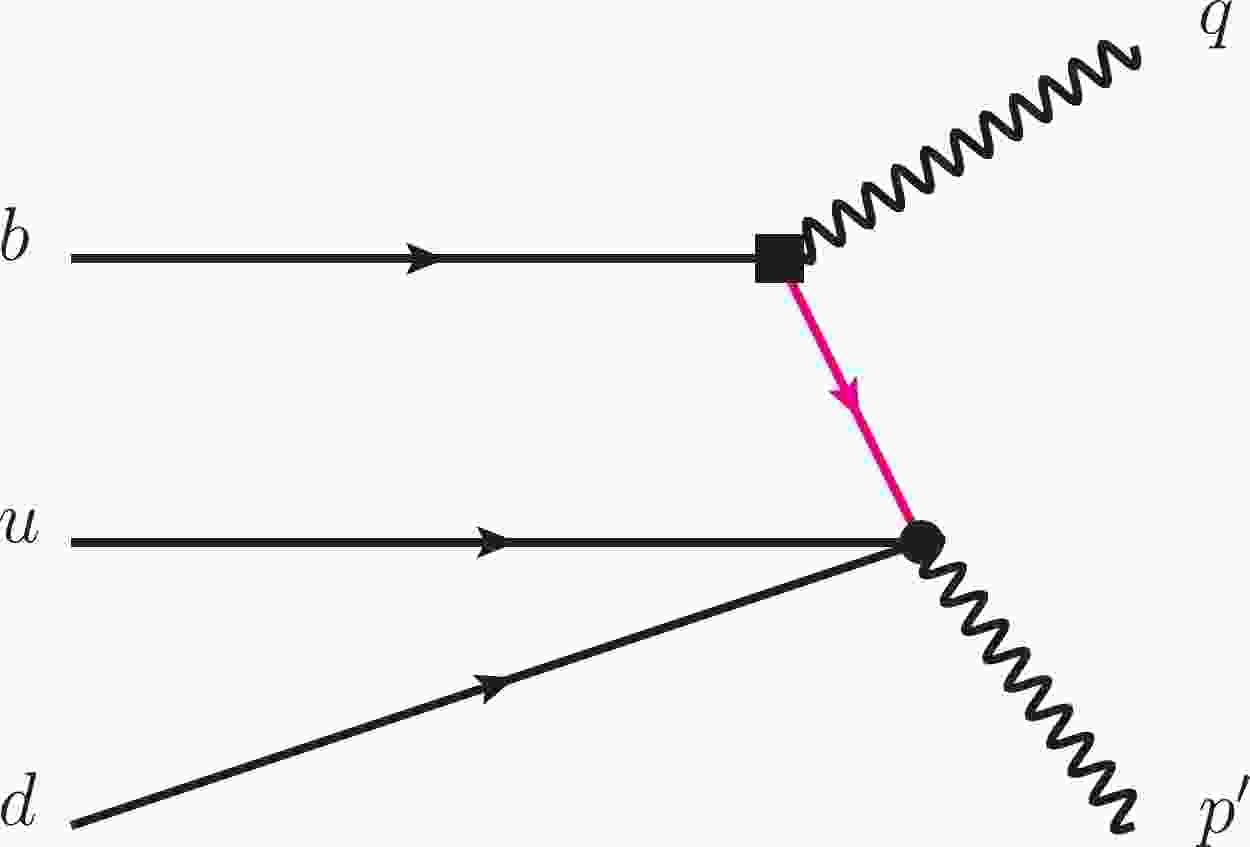
(20) From the diagram in Fig. 1, the leading-order hard kernel can be obtained.

Figure 1. (color online) Diagrammatic representation of the correlation function
$ \Pi_{\mu, a}(n \cdot p^{\prime},\bar n \cdot p^{\prime}) $ at tree level, where the black square denotes the weak transition vertex, the black blob represents the Dirac structure of the$ \Lambda_c $ -baryon current, and the pink internal line indicates the propagator of the charm quark.$ \begin{aligned}[b] T^{({\rm P},0)}_{\alpha \beta \gamma \delta}(p,q) =& -\left[C\gamma^5\right]_{\alpha\beta} \left[{\not p-\not k+m_c\over (p-k)^2-m_c^2}\gamma_\mu(I,\gamma_5)\right]_{\gamma\delta}, \\ T^{({\rm A},0)}_{\alpha \beta \gamma \delta}(p,q) =& -\left[C\gamma^5\gamma^\rho\right]_{\alpha\beta} \left[\gamma_\rho{\not p-\not k+m_c\over (p-k)^2-m_c^2}\gamma_\mu(I,\gamma_5)\right]_{\gamma\delta} . \end{aligned} $

(21) where
$ k=k_1+k_2 $ , and$ k_{1,2} $ represents the momentum of the two soft light quarks inside the$ \Lambda_b $ -baryon. Inserting the hard functions and DAs into the correlation functions, we can obtain the partonic expression of the correlation functions. Note that to match the light-like vector n and$ \bar n $ in the definition of the DAs of the$ \Lambda_b $ baryon and the momentum$ p',q $ in the parametrization of the correlation function, we must perform the replacement$ \begin{aligned}[b]&\psi(\omega)\not \bar n\to \overline{\psi}(\omega)\not \partial_{p'},\,\, \psi(\omega)\not n\to 2\psi(\omega)\not v \\&\quad-\overline{\psi}(\omega)\not \partial_{p'}\,\,{\rm or}\,\,\overline{\psi}(\omega)(2\not vv\cdot \partial_{p'}-\not \partial_{p'}), \end{aligned}$

(22) where
$\bar \psi(\omega)=\int_0^\omega \eta\psi(\eta) {\rm d}\eta$ . The obtained invariant amplitudes$ \Pi^{a}_{i} $ can be expressed by the following dispersion integral:$ \Pi^{a}_{i}(p^2 , q^2)=\frac{1}{\pi} \int^{\infty}_0 \frac{{\rm d}s}{s-p^2} {\rm Im}_s \Pi^a_i(s,q^2). $

(23) Taking advantage of the quark hadron duality ansatz, that is, equalizing the contributions from the continuum states and higher states in the hadronic expression and dispersion integral with the lower limit set as the threshold
$ s_0 $ in the partonic expression of the correlation function and performing the Borel transform, we can obtain the sum rules at leading power. For the P-type current, the sum rules of the form factors can be written as$\begin{aligned}[b] f_i^{\rm P,LP}=&-{m_{\Lambda_b}^2\over m_{\Lambda_c}(m_{\Lambda_c}+m_{\Lambda_c^\ast})\lambda^{\rm P}_{\Lambda_c^\ast}}\int_0^1 {\rm d} u\int_0^{\sigma_0}\\&\times{\sigma {\rm d}\sigma\over \bar\sigma}[\rho_{i+,a}^{\rm P}(\sigma)+m_{\Lambda_c^\ast}\rho_{i-,a}^{\rm P}(\sigma)] {\rm e}^{(m_{\Lambda_c}^2-s(\sigma))/M_B^2} ,\end{aligned} $

(24) where the nonzero spectrum densities read
$ \begin{aligned}[b] {\rho^{\rm P}_{1+,a}}=&-{1\over 4}f_{\Lambda_b}^{(1)}\left(\psi_3^{+-}+ \psi_3^{-+}\right)(m_{\Lambda_b}\sigma+m_c),\\\rho^{\rm P}_{2+,a}=&{1\over 2}f_{\Lambda_b}^{(1)}\left(\psi_3^{+-}+ \psi_3^{-+}\right)m_{\Lambda_b}\sigma, \\ \rho^{\rm P}_{2-,a}=&{-{1\over 4}f_{\Lambda_b}^{(1)}\left(\psi_3^{+-}+ \psi_3^{-+}\right)}. \end{aligned} $

(25) For the A-type current, we have
$ \begin{aligned}[b] f_i^{\rm A, LP}=&{-{\rm e}^{m_{\Lambda_c}^2/M_B^2}\over m_{\Lambda_c}(m_{\Lambda_c}+m_{\Lambda_c^\ast})\lambda^{\rm A}_{\Lambda_c^\ast}}\int_0^1 {\rm d} u\\&\times\bigg\{\int_0^{\sigma_0}{m_{\Lambda_b}^2\sigma {\rm d}\sigma\over \bar\sigma}[\rho_{i+,a}^{\rm A}(\sigma)+m_{\Lambda_c^\ast}\rho_{i-,a}^{\rm A}(\sigma)]{\rm e}^{-s(\sigma)/M_B^2} \\ &+{[\rho_{i+,b}^{\rm A}(\sigma_0)+m_{\Lambda_c^\ast}\rho_{i-,b}^{\rm A}(\sigma_0)]\over {m_{\Lambda_b}\bar \sigma_0}^2}\eta(\sigma_0){\rm e}^{-s_0/M_B^2}\\&+\int_0^{\sigma_0}{m_{\Lambda_b} {\rm d}\sigma\over {\bar\sigma}^2}{[\rho_{i+,b}^{\rm A}(\sigma)+m_{\Lambda_c^\ast}\rho_{i-,b}^{\rm A}(\sigma)]\over M_B^2} {\rm e}^{-s(\sigma)/M_B^2}\bigg\} , \end{aligned}$

(26) where the nonzero spectrum densities are given below.
$ \begin{aligned}[b] \rho^{\rm A}_{1+,a}=&-{1\over 2}f_{\Lambda_b}^{(2)}{[2(\bar \psi_4-\bar \psi_2)}+2\psi_2(2m_{\Lambda_c}v\cdot v'-m_{\Lambda_b}\sigma-m_c)\\&+(\psi_{\perp, 1}+\psi_{\perp, 2})],\,\, \rho^{\rm A}_{1-,a}=-f_{\Lambda_b}^{(2)}{\psi_2}, \\ \rho^{\rm A}_{1+,b}=& f_{\Lambda_b}^{(2)}(\bar \psi_4-\bar \psi_2)m_c(m_{\Lambda_b}\sigma+m_c),\\ \rho^{\rm A}_{1-,b}=&f_{\Lambda_b}^{(2)}{m_c}(\bar \psi_4-\bar \psi_2),\\ \rho^{\rm A}_{2+,a}=&-{2}f_{\Lambda_b}^{(2)}m_c\psi_2,\,\, \rho^{\rm A}_{2-,a}={2}f_{\Lambda_b}^{(2)}\psi_2, \\ \rho^{\rm A}_{2+,b}=&-{2}f_{\Lambda_b}^{(2)}(\bar \psi_4-\bar \psi_2)m_cm_{\Lambda_b}\sigma .\\[-10pt] \end{aligned} $

(27) The form factors
$ g_i $ can be obtained from$ f_i $ directly; therefore, we do not present explicit expressions. -
Now, we discuss the power suppressed contribution from heavy quark expansion. To achieve the target, we should replace the leading power heavy quark field in the heavy-to-light current by the NLP suppressed one in the QCD calculation, that is,
$ \bar c\Gamma h_v \to \bar c \Gamma {{\rm i}\not D\over 2m_b}h_v. $

(28) Then, the correlation function (we take the correlation function with the P-type interpolation current as an example) becomes
$\begin{aligned}\\[-8pt] \Pi^{\rm P,NLP}_{\mu, a}(q, p')= {\rm i} \int {\rm d}^4 x \, {\rm e}^{{\rm i} p' \cdot x} \, \langle 0 |T \{\epsilon^{ijk}(u^iC\gamma_5d^j)c^k(x), \bar c(0) \Gamma_a {{\rm i}\not D\over 2m_b}h_v(0) \}| \Lambda_b(v) \rangle \,.\end{aligned} $ 
(29) Contracting the charm quark field, we have
$ \Pi^{\rm P,NLP}_{\mu, a}(q, p')= {\rm i} \int{{\rm d}^4k\over (2\pi)^4}\int {\rm d}^4 x \, {{\rm i}{\rm e}^{{\rm i} (p'-k) \cdot x}\over k^2-m_c^2} \, \langle 0 |\epsilon^{ijk}(u^iC\gamma_5d^j)(\not k+m_c) \Gamma_a {{\rm i}\not D\over 2m_b}h_v(0) | \Lambda_b(v) \rangle \,, $

(30) The QCD equation of motion indicates that
$ \begin{aligned}[b] [q_1(x)\Gamma' q_2(x)] \, \Gamma \, {\overrightarrow{D}}_{\rho} \, h_v(0) =& \partial_{\rho} \left ( [q_1(x)\Gamma' q_2(x)] \, \Gamma \, h_v(0) \right ) \, + \, {\rm i} \, \int_0^1 {\rm d} u \, \bar u \,\, [q_1(x)\Gamma' q_2(x)] \,g_s \, G_{\lambda \rho}(u x) \, x^{\lambda} \, \Gamma \, h_v(0) \\ & - \, {\partial \over \partial x^{\rho}}[q_1(x)\Gamma' q_2(x)] \, \Gamma \, h_v(0) \,. \end{aligned}$

(31) The matrix element of the second term results in the convolution of the hard function and the four-point LCDA of the
$ \Lambda_b $ -baryon, which has not yet been studied; thus, we leave this part for future studies. In addition, the derivative on the gauge link will also result in an additional gluon field, which will also be neglected in this study. The correlation function then reads$ \begin{aligned}[b] \Pi^{\rm P,NLP}_{\mu, a}(q, p')\simeq& -{\rm i} {1\over 2m_b}\int{{\rm d}^4k\over (2\pi)^4}\int {\rm d}^4 x \, {{\rm e}^{{\rm i} (p'-k) \cdot x}\over k^2-m_c^2} \, \partial_\rho \langle 0 |\epsilon^{ijk}(u^iC\gamma_5d^j)(\not k+m_c) \Gamma_a \gamma^\rho h_v(0) | \Lambda_b(v) \rangle \, \\&+ {\rm i} {1\over 2m_b}\int{{\rm d}^4k\over (2\pi)^4}\int {\rm d}^4 x \, {{\rm e}^{{\rm i} (p'-k) \cdot x}\over k^2-m_c^2} \, {\partial\over \partial x^\rho} \langle 0 |\epsilon^{ijk}(u^iC\gamma_5d^j)(\not k+m_c) \Gamma_a \gamma^\rho h_v(0) | \Lambda_b(v) \rangle , \end{aligned} $ 
(32) The first term can be evaluated directly. Taking advantage of the definition of the heavy quark field in HQET, the partial derivative leads to a simple nonperturbative parameter.
$ \begin{aligned}[b]&\partial_\rho\langle 0 |\epsilon^{ijk}(u^iC\gamma_5d^j)(\not k+m_c) \Gamma_a \gamma^\rho h_v(0) | \Lambda_b(v) \rangle \\=&-{\rm i}\bar \Lambda \langle 0 |\epsilon^{ijk}(u^iC\gamma_5d^j)(\not k+m_c) \Gamma_a h_v(0) | \Lambda_b(v) \rangle\, , \end{aligned}$

(33) where the nonperturbative parameter is regarded as the mass difference between the
$ \Lambda_b $ -baryon and the b-quark for a good approximation, that is,$ \bar \Lambda\simeq m_{\Lambda_b} - m_b $ . For the second term, performing integration by parts yields an additional$ \omega=v\cdot (p'-k) $ in the integrand. Combining these two parts together, we have$\begin{aligned}[b]\Pi^{\rm P,NLP}_{\mu, a}(q, p')=& -{\bar \Lambda\over 2m_b}\Pi^{\rm P,LP}_{\mu, a}(q, p')-{1\over 2m_b}\int \omega' {\rm d} \omega^{\prime}\\&\times \int_0^1 {\rm d}u \, T^{\rm (P,0)}_{\alpha \beta \gamma \delta}( p^{\prime}, q, u\omega^{\prime}, \bar u\omega^{\prime})\, \Phi_{\Lambda_b}^{ \, \alpha \beta \delta}(\omega^{\prime}, u). \end{aligned}$

(34) Finally, we arrive at the sum rules of the form factors at NLP, which are expressed as
$\begin{aligned}[b] f_i^{\rm P,NLP} =& {m_{\Lambda_b}^2\over m_{\Lambda_c}(m_{\Lambda_c}+m_{\Lambda_c^\ast})\lambda^P_{\Lambda_c}}\int_0^1{\rm d} u\int_0^{\sigma_0}{\bar \Lambda+\sigma m_{\Lambda_b}\over 2m_b}\\&\times{\sigma {\rm d}\sigma\over \bar\sigma}[\rho_{i+,a}^{\rm P}(\sigma)+m_{\Lambda_c}\rho_{i-,a}^{\rm P}(\sigma)] {\rm e}^{(m_{\Lambda_c}^2-s(\sigma))/M_B^2} ,\end{aligned} $

(35) From the above result, we can see that the power suppressed contribution considered in this study involves the addition of a factor
$ (\bar\Lambda-\sigma m_{\Lambda_b})/( 2m_b) $ in the integrand of the leading power contribution if the P-type interpolation current is employed. For the A-type interpolation current, we must perform a more complicated modification because$ \bar \psi_i(\omega) $ exists in the integrand. The specific operation is as follows: In the spectrum density$\rho_{i\pm,a(b)}^{\rm A}$ , we multiply$ (\Lambda-\sigma m_{\Lambda_b})/( 2m_b) $ to the terms proportional to$ \psi_i(\sigma) $ and replace$ \bar \psi_i $ by$ \tilde{\psi}_i/m_b $ , where$ \tilde{\psi}_i(\omega) $ is defined as$\tilde{\psi}_i(\omega)= \displaystyle\int_0^\omega\eta^2\psi_i(\eta){\rm d}\eta$ . -
The DAs of the
$ \Lambda_b $ -baryon are the fundamental ingredients of the LCSR of the form factors considered in this study; however, they are not well established to date owing to a poor understanding of QCD inside heavy baryon systems. In [55–57], several different models of the LCDAs of the$ \Lambda_b $ baryon have been suggested up to twist-4 (not including the twist of the heavy quark field). We consider the following three different models. The first is obtained from calculation with QCDSR [56] and thus is known as the QCDSR model. The specific form of the LCDAs$ \psi_2(\omega, u),\psi_3^{+-}(\omega, u), \psi_3^{-+}(\omega, u), \psi_4(\omega, u) $ reads$ \begin{aligned}[b] \psi_2(\omega, u) =& \frac{15}{2{\cal{N}}}\omega^2 u(1-u)\int^{s^{\Lambda_b}_0}_{\omega/2}{\rm d}s\ {\rm e}^{-s/\tau} (s-\omega/2), \\ \psi^{+-}_{3}(\omega,u) =& \frac{15}{{\cal{N}}}\omega u\int^{s^{\Lambda_b}_0}_{\omega/2}{\rm d}s\ {\rm e}^{-s/\tau}(s-\omega/2)^2 ,\\ \psi^{-+}_{3}(\omega,u) =& \frac{15}{{\cal{N}}}\omega (1-u)\int^{s^{\Lambda_b}_0}_{\omega/2}{\rm d}s\ {\rm e}^{-s/\tau}(s-\omega/2)^2 ,\\ \psi_4(\omega,u) =& \frac{5}{{\cal{N}}}\int^{s^{\Lambda_b}_0}_{\omega/2}{\rm d}s\ {\rm e}^{-s/\tau}(s-\omega/2)^3 \end{aligned} $

(36) where
${\cal{N}}=\displaystyle\int^{s^{\Lambda_b}_0}_0 {\rm d} s\ s^5 {\rm e}^{-s/\tau}$ , τ is the Borel parameter, which is constrained in the interval$ 0.4<\tau<0.8 $ GeV, and$ {s^{\Lambda_b}_0}=1.2 $ GeV is the continuum threshold. The other two phenomenological models are proposed in [55] and are known as the exponential model and free parton model. For the exponential model,$ \begin{aligned}[b] \psi_2(\omega,u) =& \frac{\omega^2 u(1-u)}{\omega^4_0}{\rm e}^{-\omega/\omega_0}, \\ \psi^{+-}_3(\omega, u) =& \frac{2\omega u}{\omega^3_0}{\rm e}^{-\omega/\omega_0}, \\ \psi^{-+}_3(\omega, u) =& \frac{2\omega (1-u)}{\omega^3_0}{\rm e}^{-\omega/\omega_0}, \\ \;\;\psi_4(\omega, u) =& \frac{1}{\omega^2_0}{\rm e}^{-\omega/\omega_0}, \end{aligned} $

(37) where
$ \omega_0=0.4\pm 0.1 $ GeV measures the average energy of the two light quarks inside the$ \Lambda_b $ -baryon. The DAs in the free-parton model take the following form:$ \begin{aligned}[b] \psi_2(\omega, u) =& \frac{15\omega^2 u(1-u)(2\bar{\Lambda}-\omega)}{4\bar{\Lambda}^5}\theta(2\bar{\Lambda}-\omega), \\ \psi^{+-}_3(\omega, u) =& \frac{15\omega u (2\bar{\Lambda}-\omega)^2}{4\bar{\Lambda}^5}\theta(2\bar{\Lambda}-\omega), \\ \psi^{-+}_3(\omega, u) =& \frac{15\omega (1-u) (2\bar{\Lambda}-\omega)^2}{4\bar{\Lambda}^5}\theta(2\bar{\Lambda}-\omega), \\ \psi_4(\omega, u) =& \frac{5(2\bar{\Lambda}-\omega)^3}{8\bar{\Lambda}^5}\theta(2\bar{\Lambda}-\omega), \end{aligned} $

(38) where
$ \theta(2\bar{\Lambda}-\omega) $ is the step-function, and$\bar{\Lambda}=m_{\Lambda_b}- m_b\approx 1\pm0.2$ GeV. The first-order terms of the light-cone are not significant numerically; however, they are required to guarantee gauge invariance. In this study, the DAs of these terms are given by$ \begin{aligned}[b] \psi^{+-}_{\perp, 1}(\omega, u) =& \psi^{-+}_{\perp, 2}=\psi^{(1)}_{\perp, 3}=\psi^{(2)}_{\perp, 3}=\frac{\omega^2 u(1-u)}{\omega_0^3} {\rm e}^{-\omega/\omega_0}, \\ \psi^{-+}_{\perp, 1}(\omega, u) =& \frac{\omega u}{\omega_0^2} {\rm e}^{-\omega/\omega_0}, \\ \psi^{+-}_{\perp, 2}(\omega, u) =& \frac{\omega (1-u)}{\omega_0^2} {\rm e}^{-\omega/\omega_0}, \\ \psi^{(1)}_{\perp, Y}(\omega, u) =& \frac{\omega u(\omega_0-\omega(1-u))}{2\omega_0^3}{\rm e}^{-\omega/\omega_0}, \\ \psi^{(2)}_{\perp, Y}(\omega, u) =& \frac{\omega (1-u)(\omega_0-\omega u)}{2\omega_0^3}{\rm e}^{-\omega/\omega_0}, \end{aligned} $

(39) where
$ \omega_0=0.4\pm0.1 $ GeV. The numerical values of the other parameters, such as the masses of the corresponding baryons, quark masses, coupling parameters of the baryons, Borel mass, and threshold parameters, are listed in Table 1. In this table, we use$\rm\overline{MS}$ mass for the charm quark, which appears in the partonic evaluation of the correlation functions. For the bottom quark mass, we take advantage of the potential subtraction (PS) mass for the b-quark because it appears in the heavy quark expansion and the PS mass is less ambiguous than the pole mass.$ m_b^{\rm PS} $ 

4.53 GeV [59] $ |V_{cb}| $ 

4.1 $ \times10^{-2} $ [60]

$ m_{\Lambda_b} $ 

5.620 GeV [60] $ m_{\Lambda_c} $ 

2.286 GeV [60] $ s_0 $ 

$ 10\pm 0.5 $ GeV2 [37]

$ M^2 $ 

$ 7.5\pm 2.5 $ GeV2 [37]

$ f^{(1)}_{\Lambda_b} $ 

$ 0.030\pm 0.005 $ GeV3 [37]

$ f^{(2)}_{\Lambda_b} $ 

$ 0.03 \pm 0.003 $ GeV3 [37]

$ \lambda^{A}_{\Lambda_c} $ 

$ (1.51\pm0.35)\times 10^{-2} $ GeV2

$ \lambda^{P}_{\Lambda_c} $ [37]

$ (1.19\pm0.19)\times 10^{-2} $ GeV2 [37]

Table 1. Imput parameters.
Because LCSR are valid only at a small
$ q^2 $ , we first present the results of the form factors$ f_1 $ and$ f_2 $ at$ q^2=0 $ , which are lsited in Table 2. To highlight the power suppressed contribution from heavy quark expansion, both the leading power contribution and NLP contribution are listed for comparison. It is clear that the NLP contribution can reduce the leading power contribution by approximately 20%, which will significantly change the results of the physical observables. We should note that the power corrections considered in this paper are preliminary, and it is necessary to perform a more careful treatment of the NLP contributions. In this table, the form factors$ f_1(0) $ and$ f_2(0) $ are evaluated with both P-type and A-type interpolation currents. The results indicate that the A-type current leads to larger results for all three models of the LCDAs of the$ \Lambda_b $ -baryon. In general, the results are consistent within the error area. The total uncertainties shown in this table are obtained by varying separate input parameters within their ranges and adding the resulting separate uncertainties of the form factors in the quadrature. The results from the QCDSR model and free parton model of$ \Lambda_b $ LCDAs are highly consistent, and the results from the exponential model are low for both A-type and P-type currents. The result of the form factor$ f_3(0) $ still satisfies$ f_3(0)=0 $ , which is expected in the heavy b-quark limit. Although we consider the power correction from heavy quark expansion, it does not yield a nonzero contribution to$ f_3(0) $ . The relations between the form factors displayed in Eq. (2), which originate from heavy quark symmetry, are still valid, as shown by the numerical results in Table 2. In Table 3, we present the predictions of the form factor$ f_i $ at$ q^2=0 $ from the light-front quark model [24, 61], relativistic quark model [22], covariant constituent quark model [62], QCDSR, [36] and lattice QCD simulation [20], along with our results. The lattice simulation is valid at a large$ q^2 $ . Here, the prediction depends on the extrapolation model and is smaller than other predictions, which leads to semileptonic decay branching ratios that are too small compared with experimental measurements. The different predictions are, in general, consistent with each other if the uncertainties are considered. In our calculation, there are two preferable scenarios: the A-type interpolation current along with the exponential model of the DAs of$ \Lambda_b $ , and the P-type interpolation current along with the QCDSR model or free parton model of the DAs of$ \Lambda_b $ . Therefore, it is difficult to distinguish different models or the interpolation current from the predictions of the form factors from the current calculation. The form factors$ g_i $ are directly related to$ f_i $ ; hence, we do not provide further discussions.Model $ f^{\rm LP}_1 $ 

$ f^{\rm NLP}_1 $ 

$ f^{\rm LP+NLP}_1 $ 

$ f^{\rm LP}_2 $ 

$ f^{\rm NLP}_2 $ 

$ f^{\rm LP+NLP}_2 $ 

A-type current QCDSR $ 0.977 $ 

$ -0.188 $ 

$ 0.789\pm 0.243 $ 

$ -0.303 $ 

$ 0.059 $ 

$ -0.244\pm 0.076 $ 

Exponential $ 0.859 $ 

$ -0.162 $ 

$ 0.697\pm0.297 $ 

$ -0.265 $ 

$ 0.050 $ 

$ -0.215\pm0.094 $ 

Free parton $ 0.931 $ 

$ -0.182 $ 

$ 0.749\pm0.339 $ 

$ -0.287 $ 

$ 0.057 $ 

$ -0.230\pm0.108 $ 

P-type current QCDSR $ 0.854 $ 

$ -0.168 $ 

$ 0.686\pm0.169 $ 

$ -0.289 $ 

$ 0.060 $ 

$ -0.229\pm0.059 $ 

Exponential $ 0.711 $ 

$ -0.137 $ 

$ 0.574\pm0.214 $ 

$ -0.231 $ 

$ 0.047 $ 

$ -0.184\pm0.061 $ 

Free parton $ 0.851 $ 

$ -0.171 $ 

$ 0.680\pm0.248 $ 

$ -0.300 $ 

$ 0.063 $ 

$ -0.237\pm0.079 $ 

$ g^{\rm LP}_1 $ 

$ g^{\rm NLP}_1 $ 

$ g^{\rm LP+NLP}_1 $ 

$ g^{\rm LP}_2 $ 

$ g^{\rm NLP}_2 $ 

$ g^{\rm LP+NLP}_2 $ 

A-type current QCDSR $ 0.675 $ 

$ -0.130 $ 

$ 0.545\pm0.167 $ 

$ -0.303 $ 

$ 0.059 $ 

$ -0.244\pm0.076 $ 

Exponential $ 0.594 $ 

$ -0.112 $ 

$ 0.482\pm0.203 $ 

$ -0.265 $ 

$ 0.050 $ 

$ -0.215\pm0.094 $ 

Free parton $ 0.644 $ 

$ -0.125 $ 

$ 0.519\pm0.231 $ 

$ -0.287 $ 

$ 0.057 $ 

$ -0.230\pm0.108 $ 

P-type current QCDSR $ 0.565 $ 

$ -0.108 $ 

$ 0.457\pm0.111 $ 

$ -0.289 $ 

$ 0.060 $ 

$ -0.229\pm0.059 $ 

Exponential $ 0.480 $ 

$ -0.090 $ 

$ 0.390\pm0.155 $ 

$ -0.231 $ 

$ 0.047 $ 

$ -0.184\pm0.061 $ 

Free parton $ 0.551 $ 

$ -0.108 $ 

$ 0.443\pm0.171 $ 

$ -0.300 $ 

$ 0.063 $ 

$ -0.237\pm0.079 $ 

Table 2. Form factors
$f^{\rm P}_i(0)$ and$f^{\rm A}_i(0)$ at$ q^2=0 $ .$ f_1(0) $ 

$ f_2(0) $ 

$ f_3(0) $ 

$ g_1(0) $ 

$ g_2(0) $ 

$ g_3(0) $ 

This study (A-type) QCDSR model 0.789 −0.244 0 0.545 −0.244 0 Exponential model 0.697 −0.215 0 0.482 −0.215 0 Free parton model 0.749 −0.230 0 0.519 −0.230 0 This study (P-type) QCDSR model 0.686 −0.229 0 0.457 −0.229 0 Exponential model 0.574 −0.184 0 0.390 −0.184 0 Free parton model 0.680 −0.237 0 0.443 −0.237 0 QCDSR [36] 0.604 −0.101 −0.059 0.456 −0.124 0.080 LFQM [24] 0.638 −0.107 −0.036 0.500 −0.100 0.028 LFQM [61] 0.669 −0.160 −0.033 0.478 −0.170 0.053 RQM [22] 0.719 −0.212 −0.025 0.521 −0.279 0.091 CCQM [62] 0.704 −0.133 −0.035 0.531 −0.141 0.042 LQCD [20] 0.558 −0.174 −0.010 0.388 −0.210 0.082 Table 3. Results of the form factor at
$ q^2=0 $ of this study are compared with those of other methods.To predict the experimental observables, we extrapolate our results at small
$ q^2 $ ($0\leq 5~{\rm GeV^2}$ ) across the entire physical region. To this end, we employ simplified z-series parametrization [63] based on conformal mapping,$ z(q^2, t_0) = \frac{\sqrt{t_+-q^2}-\sqrt{t_+-t_0}}{\sqrt{t_+-q^2}+\sqrt{t_+-t_0}},\, $

(40) which transforms the cut
$ q^2 $ -plane onto the disk$ |z(q^2, t_0)| \leq 1 $ on the complex z-plane. We choose the parameter$ t_{\pm} $ to be$ t_{\pm}=(m_{\Lambda_b}\pm m_{\Lambda_c})^2 $ and$t_0=t_+-\sqrt{t_+-t_{-}}\times \sqrt{t_+-t_{\min}}$ to reduce the interval of z after mapping$ q^2 $ to z with the interval$ t_{\rm min}<q^2<t_{-} $ . In the numerical analysis, we take$t_{\min}= -6$ GeV2. Keeping the series expansion of the form factors to the first power of the z-parameter, we propose the following parameterizations:$ \begin{aligned}[b] f_i(q^2) =& \frac{f_i(0)}{ 1-q^2/m_{B_c^{\ast}(1^-)}^2} \, \left \{ 1 + a_1^{i} \, \left [ z(q^2, t_0) - z(0, t_0) \right ] \right \} \, \\ g_i(q^2) =& \frac{g_i(0)}{1-q^2/m_{B_c^{\ast}(1^+)}^2} \, \left \{ 1 + b_1^{i} \, \left [ z(q^2, t_0) - z(0, t_0) \right ] \right \}, \, \end{aligned} $

(41) where the masses of
$ {B_c^{\ast}(1^-)} $ and$ {B_c^{\ast}(1^+)} $ appear in the pole factor but are not measured. There are several theoretical estimations of these masses, and we adopt$m_{B_c^{\ast}(1^-)}=$ 6.336 GeV and$m_{B_c^{\ast}(1^+)}=6.745~{\rm GeV}$ [58]. The fitted results of$ a_1^i, b_1^i $ are presented in Table 4. Because the form factors are extrapolated across the entire physical region, we plot the$ q^2 $ -dependence of the form factors with the different DAs of the$ \Lambda_b $ -baryon in Fig. 2. The uncertainties shown in the bands are obtained by adding the resulting separate uncertainties from$ f_i(0),a_i,b_i $ in the quadrature.Model $ f_1 $ 

$ f_2 $ 

$ g_1 $ 

$ g_2 $ 

A-type current QCDSR $ f(0) $ 

$ 0.789\pm0.243 $ 

$ -0.244\pm0.076 $ 

$ 0.545\pm0.167 $ 

$ -0.244\pm0.076 $ 

$ a_1 $ 

$ -6.92\pm2.7 $ 

$ -14.95\pm2.9 $ 

$ -4.15\pm2.8 $ 

$ -15.93\pm2.9 $ 

Exponential $ f(0) $ 

$ 0.697\pm0.297 $ 

$ -0.215\pm0.094 $ 

$ 0.482\pm0.203 $ 

$ -0.215\pm0.094 $ 

$ a_1 $ 

$ -6.21\pm3.1 $ 

$ -14.65\pm2.6 $ 

$ -3.26\pm2.6 $ 

$ -15.63\pm2.5 $ 

Free parton $ f(0) $ 

$ 0.749\pm0.339 $ 

$ -0.230\pm0.108 $ 

$ 0.519\pm0.231 $ 

$ -0.230\pm0.108 $ 

$ a_1 $ 

$ -10.32\pm2.9 $ 

$ -18.91\pm2.4 $ 

$ -7.37\pm3.0 $ 

$ -19.94\pm2.3 $ 

P-type current QCDSR $ f(0) $ 

$ 0.686\pm0.169 $ 

$ -0.229\pm0.059 $ 

$ 0.457\pm0.111 $ 

$ -0.229\pm0.059 $ 

$ b_1 $ 

$ -5.74\pm2.2 $ 

$ -11.00\pm2.4 $ 

$ -3.96\pm2.1 $ 

$ -11.93\pm2.4 $ 

Exponential $ f(0) $ 

$ 0.574\pm0.214 $ 

$ -0.184\pm0.061 $ 

$ 0.390\pm0.155 $ 

$ -0.184\pm0.061 $ 

$ b_1 $ 

$ -6.25\pm3.1 $ 

$ -12.68\pm2.6 $ 

$ -4.04\pm2.8 $ 

$ -13.62\pm2.6 $ 

Free parton $ f(0) $ 

$ 0.680\pm0.248 $ 

$ -0.237\pm0.079 $ 

$ 0.443\pm0.171 $ 

$ -0.237\pm0.079 $ 

$ b_1 $ 

$ -6.92\pm2.6 $ 

$ -12.21\pm2.8 $ 

$ -4.96\pm2.8 $ 

$ -13.16\pm2.7 $ 

Table 4. Fitted results of
$ a_1,b_1 $ for the form factors$ F^{p}_i $ ,$ F^{A}_i $ ,$ G^{p}_i $ , and$ G^{p}_i $ .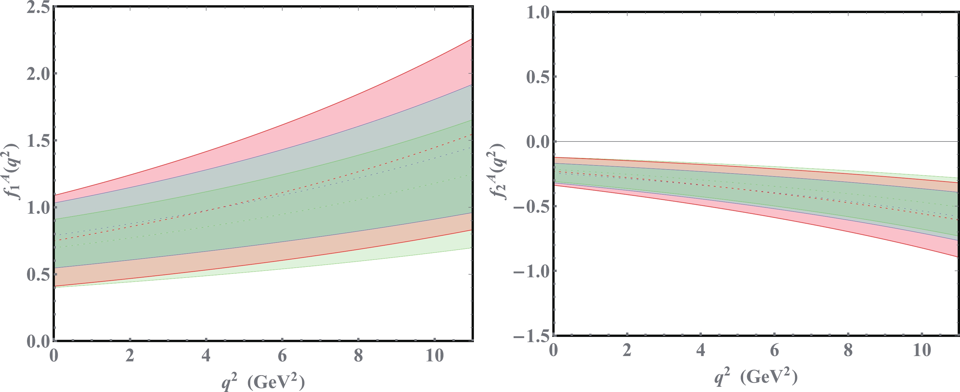
Figure 2. (color online) Form factors
$ f_1(q^2) $ and$ f_2(q^2) $ from the A-type interpolation current. The blue, green, and red bands denote the form factors from the QCDSR , exponential, and free parton models, respectively.In the following, we aim at exploring the phenomenological applications of the obtained
$ \Lambda_b \to \Lambda_c $ form factors. These serve as fundamental ingredients for the theory description of$ \Lambda_b \to \Lambda_c \ell \nu $ decays, which are regarded as a good platform to further investigate the$ R_{D(D^\ast)} $ anomaly. To calculate phenomenological observables, such as the branching ratios, and forward backward asymmetries, it is convenient to introduce helicity amplitudes, which are defined by$ H^{V,A}_{\lambda_{\Lambda_c},\lambda_{W^-} }=\epsilon^{\dagger\mu}(\lambda_{W^-})\langle \Lambda_c,\lambda_{\Lambda_c}|V(A)|\Lambda_b, \lambda_{\Lambda_b}\rangle , $

(42) where
$ \lambda_{\Lambda_b}, \lambda_{\Lambda_c}, \lambda_{W^-} $ denote the helicity of the$ \Lambda_b $ baryon,$ \Lambda_c $ baryon, and off-shell$ W^- $ , respectively, which mediate semileptonic decays. The helicity amplitudes$ H^{V,A}_{\lambda_{\Lambda_c},\lambda_{W^-}} $ can be expressed as functions of the form factors$ \begin{aligned}[b] H^{V}_{\frac{1}{2},0} =& \frac{\sqrt{Q_-}}{\sqrt{q^2}}\Big[M_+F_1(q^2)- \frac{q^2}{m_{\Lambda_b}}F_2(q^2)\Big],\\ H^{A}_{\frac{1}{2},0}=&\frac{\sqrt{Q_+}}{\sqrt{q^2}}\Big[M_-G_1(q^2)+ \frac{q^2}{m_{\Lambda_b}}G_2(q^2)\Big] , \\ H^{V}_{\frac{1}{2},1} =& \sqrt{2Q_-}\Big[F_1(q^2)- \frac{M_+}{m_{\Lambda_b}}F_2(q^2)\Big] , \\ H^{A}_{\frac{1}{2},1}=&\sqrt{2Q_+}\Big[G_1(q^2)+ \frac{M_-}{m_{\Lambda_b}}G_2(q^2)\Big] , \\ H^{V}_{\frac{1}{2},t} =& \frac{\sqrt{Q_+}}{\sqrt{q^2}}\Big[M_-F_1(q^2)+ \frac{q^2}{m_{\Lambda_b}}F_3(q^2)\Big], \\ H^{A}_{\frac{1}{2},t}=&\frac{\sqrt{Q_-}}{\sqrt{q^2}}\Big[M_+G_1(q^2)- \frac{q^2}{m_{\Lambda_b}}G_3(q^2)\Big] .\end{aligned} $

(43) where
$ Q_{\pm} $ is defined as$ Q_{\pm}=(m_{\Lambda_b}\pm m_{\Lambda_c})^2-q^2 $ , and$ M_{\pm}= m_{\Lambda_b} \pm m_{\Lambda_c} $ . The negative helicities can be obtained by$ H^{V}_{-\lambda_{\Lambda_c},-\lambda_{W^-}}=H^{V}_{\lambda_{\Lambda_c},\lambda_{W^-}},\ \ \ H^{A}_{-\lambda_{\Lambda_c},-\lambda_{W^-}}=-H^{A}_{\lambda_{\Lambda_c},\lambda_{W^-}} . $

(44) The total helicity amplitudes are then written as
$ H_{\lambda_{\Lambda_c},\lambda_{W^-}}=H^{V}_{\lambda_{\Lambda_c},\lambda_{W^-}}-H^{A}_{\lambda_{\Lambda_c},\lambda_{W^-}}, $

(45) which are consistent with the results in [64]. The differential angular distribution for the
$ \Lambda_b \rightarrow \Lambda_c\ell \bar{\nu}_\ell $ has the following form$ \frac{{\rm d}\Gamma(\Lambda_b \rightarrow \Lambda_c \ell^-\bar{\nu}_\ell)}{{\rm d}q^2 {\rm d} \cos\theta_\ell}=\frac{G_{\rm F}^2|V_{cb}|^2q^2|\vec{p^\prime}|}{512\pi^3m^2_{\Lambda_b}}\Bigg(1-\frac{m^2_\ell}{q^2}\Bigg)^2 \Bigg(A_1+\frac{m_\ell^2}{q^2}A_2\Bigg), $

(46) where
$G_{\rm F}$ is the Fermi constant,$ V_{cb} $ is the CKM matrix element,$ m_\ell $ is the lepton mass ($ \ell=e,\mu,\tau $ ),$ \theta_\ell $ is the angle between the three-momentum of the final$ \Lambda_c $ baryon and the lepton in the$ q^2 $ rest frame,$ \vec{p^\prime} $ is the three-momentum of the$ \Lambda_c $ -baryon, and the amplitudes$ A_i $ are defined as$ \begin{aligned}[b] A_1 =& 2\sin^2\theta_\ell(H^2_{1/2,0}+H^2_{-1/2,0})+(1-\cos \theta_\ell)^2H^2_{1/2,1}\\&+(1+\cos\theta_\ell)^2H^2_{-1/2,-1} , \\ A_2 =& 2\cos^2\theta_\ell(H^2_{1/2,0}+H^2_{-1/2,0})\\&+\sin^2 \theta_\ell(H^2_{1/2,1}+H^2_{-1/2,-1})+2(H^2_{1/2,t}+H^2_{-1/2,t}) \\ & -4\cos\theta_\ell(H_{1/2,t}H_{1/2,0}+H_{-1/2,t}H_{-1/2,0}). \end{aligned} $

(47) The differential decay rate can be obtained by integrating with respect to
$ \cos\theta_l $ $ \frac{{\rm d}\Gamma(\Lambda_b\rightarrow \Lambda_c\ell^-\bar{\nu}_l)}{{\rm d}q^2}=\int^1_{-1}\frac{{\rm d}\Gamma(\Lambda_b \rightarrow \Lambda_c\ell^-\bar{\nu}_\ell)}{{\rm d} q^2 {\rm d} \cos\theta_\ell}{\rm d}\cos\theta_\ell. $

(48) In addition, other observables, such as leptonic forward-backward asymmetry (
$A_{FB}$ ), final state hadron polarization ($P_{B}$ ), and lepton polarization ($ P_\ell $ ), are defined as$\begin{aligned}[b] A_{FB}(q^2) =&\frac{\displaystyle\int^1_0 \dfrac{{\rm d}\Gamma}{{\rm d}q^2{\rm d}\cos\theta_\ell}{\rm d}\cos\theta_l-\displaystyle\int^0_{-1} \dfrac{{\rm d}\Gamma}{{\rm d}q^2{\rm d}\cos\theta_\ell}{\rm d}\cos\theta_\ell}{\displaystyle\int^1_0 \dfrac{{\rm d}\Gamma}{{\rm d}q^2 {\rm d}\cos\theta_\ell}{\rm d}\cos\theta_\ell+\displaystyle\int^0_{-1} \dfrac{{\rm d}\Gamma}{{\rm d}q^2{\rm d}\cos\theta_\ell}{\rm d}\cos\theta_\ell} , \\ P_B(q^2) =&\frac{{\rm d}\Gamma^{\lambda_{\Lambda_c}=1/2}/{\rm d}q^2-{\rm d}\Gamma^{\lambda_{\Lambda_c}=-1/2}/{\rm d}q^2}{{\rm d}\Gamma/{\rm d}q^2} , \\ P_\ell(q^2) =&\frac{{\rm d}\Gamma^{\lambda_\ell=1/2}/{\rm d}q^2-{\rm d}\Gamma^{\lambda_\ell=-1/2}/{\rm d}q^2}{{\rm d}\Gamma/{\rm d}q^2}, \end{aligned} $

(49) and the differential widths with definite polarization of the final state can be written as
$ \begin{aligned}[b] \frac{{\rm d}\Gamma^{\lambda_{\Lambda_c}=1/2}}{{\rm d}q^2} =&\frac{4m^2_l}{3q^2}\Big(H^2_{1/2,1}+H^2_{1/2,0}+3H^2_{1/2,t}\Big)\\&+\frac{8}{3}\Big(H^2_{1/2,0}+H^2_{1/2,1}\Big) , \\ \frac{{\rm d}\Gamma^{\lambda_{\Lambda_c}=-1/2}}{{\rm d}q^2} =&\frac{4m^2_l}{3q^2}\Big(H^2_{-1/2,-1}+H^2_{-1/2,0}+3H^2_{-1/2,t}\Big)\\&+\frac{8}{3}\Big(H^2_{-1/2,0}+H^2_{-1/2,-1}\Big) , \\ \frac{{\rm d}\Gamma^{\lambda_\ell=1/2}}{{\rm d}q^2} =&\frac{m^2_l}{q^2}\Big[\frac{4}{3}\Big(H^2_{1/2,1}+H^2_{1/2,0}+H^2_{-1/2,-1}+H^2_{-1/2,0}\Big)\\&+4\Big(H^2_{1/2,t}+H^2_{-1/2,t}\Big)\Big] , \\ \frac{{\rm d}\Gamma^{\lambda_\ell=-1/2}}{{\rm d}q^2} =&\frac{8}{3}\Big(H^2_{1/2,1}+H^2_{1/2,0}+H^2_{-1/2,-1}+H^2_{-1/2,0}\Big). \end{aligned} $

(50) The numerical results of the relevant observables in the semi-leptonic
$ \Lambda_b \rightarrow \Lambda_c\ell\nu $ decay are presented in Table 5, where both the A-type and P-type interpolation currents are considered. Three different models of the$ \Lambda_b $ -baryon are employed in the calculation so that they can be compared with the experimental results to determine which is preferable. The central value of the life time of$ \Lambda_b $ is set as$ \tau_{\Lambda_b}=1.470 $ ps, and the CKM matrix element$ |V_{cb}| $ is presented in Table 1. From Table 5, we can see that the integrated branching ratio for the semi-leptonic decay$ \Lambda_b \rightarrow \Lambda_c \ell^-\nu $ from the P-type interpolating current is slight smaller than that from the A-type current. Compared with the experimental data${\rm Br}(\Lambda_b \rightarrow \Lambda_c\ell\nu)= 6.2^{+1.4}_{-1.3}\%$ , the prediction of A-type operators seems more consistent with the data if the exponential model is adopted. Note that our results are from the tree level calculation of the leading power contribution in the heavy quark limit plus a rough estimation of the power corrections from heavy quark expansion. Hence, this conclusion is preliminary, and a more careful study is required to distinguish between different models of$ \Lambda_b $ DAs and the interpolation currents. The numerical results of leptonic forward-backward asymmetry ($A_{FB}$ ), final hadron polarization ($P_{B}$ ), and lepton polarization ($ P_\ell $ ) are also presented in Table 5. Because these observables are not sensitive to the form factors in the small$ q^2 $ region, the predictions from different LCDA models and interpolation currents are similar. To compare our results and the prediction from other methods, we present numerical results from various studies in Table 6. We can see that the integrated branching ratios from various studies do not significantly deviate from each other, whereas the other observables are more sensitive to different approaches, which can serve as the basis to distinguish between different methods. We also present the ratio of the branching ratio$ R_{\Lambda_c} $ in Table 5. It is not sensitive to the interpolation current and the model of the LCDAs of$ \Lambda_b $ , and the central value of our prediction is slightly smaller than that of a recent study [65]. However, it is consistent with the recent LHCb reported result$ R(\Lambda_c) =0.242 \pm 0.026 \pm 0.040 \pm 0.059 $ [66]. Furthermore, our predictions for the branching ratios have a large uncertainty. To improve the theoretical precision, we can make the following improvements: reducing the uncertainty on the parameters inside the DAs of the heavy baryon via a global fit or lattice calculation and including loop corrections and more power corrections.Model l Br( $ \times 10^{-2} $ )

$\langle A_{FB}\rangle$ 

$\langle P_{B}\rangle$ 

$\langle P_\ell\rangle$ 

$ R_{\Lambda_c} $ 

A-type current QCDSR e $ 7.68\pm3.66 $ 

$ 0.18\pm0.02 $ 

$ -0.87\pm0.15 $ 

$ -1.00\pm0.00 $ 

$ 0.273\pm0.013 $ 

μ $ 7.65\pm3.65 $ 

$ 0.17\pm0.02 $ 

$ -0.87\pm0.15 $ 

$ -0.98\pm0.00 $ 

τ $ 2.09\pm1.05 $ 

$ -0.05\pm0.03 $ 

$ -0.79\pm0.14 $ 

$ -0.29\pm0.17 $ 

Exponential e $ 5.81\pm3.78 $ 

$ 0.18\pm0.03 $ 

$ -0.88\pm0.20 $ 

$ -1.00\pm0.00 $ 

$ 0.268\pm0.015 $ 

μ $ 5.78\pm3.77 $ 

$ 0.17\pm0.03 $ 

$ -0.87\pm0.20 $ 

$ -0.98\pm0.01 $ 

τ $ 1.55\pm1.06 $ 

$ -0.05\pm0.05 $ 

$ -0.79\pm0.19 $ 

$ -0.29\pm0.24 $ 

Free-parton e $ 7.85\pm5.43 $ 

$ 0.18\pm0.03 $ 

$ -0.86\pm0.22 $ 

$ -1.00\pm0.00 $ 

$ 0.288\pm0.016 $ 

μ $ 7.82\pm5.41 $ 

$ 0.18\pm0.03 $ 

$ -0.86\pm0.22 $ 

$ -0.98\pm0.01 $ 

τ $ 2.25\pm1.62 $ 

$ -0.04\pm0.05 $ 

$ -0.78\pm0.21 $ 

$ -0.30\pm0.25 $ 

P-type current QCDSR e $ 5.42\pm2.06 $ 

$ 0.18\pm0.02 $ 

$ -0.88\pm0.12 $ 

$ -1.00\pm0.00 $ 

$ 0.270\pm0.011 $ 

μ $ 5.40\pm2.05 $ 

$ 0.17\pm0.02 $ 

$ -0.87\pm0.12 $ 

$ -0.98\pm0.00 $ 

τ $ 1.46\pm0.58 $ 

$ -0.05\pm0.03 $ 

$ -0.79\pm0.11 $ 

$ -0.29\pm0.14 $ 

Exponential e $ 3.93\pm2.37 $ 

$ 0.18\pm0.03 $ 

$ -0.87\pm0.18 $ 

$ -1.00\pm0.00 $ 

$ 0.271\pm0.014 $ 

μ $ 3.91\pm2.36 $ 

$ 0.17\pm0.03 $ 

$ -0.87\pm0.18 $ 

$ -0.98\pm0.01 $ 

τ $ 1.06\pm0.67 $ 

$ -0.05\pm0.04 $ 

$ -0.79\pm0.17 $ 

$ -0.29\pm0.21 $ 

Free-parton e $ 5.36\pm3.15 $ 

$ 0.19\pm0.03 $ 

$ -0.88\pm0.18 $ 

$ -1.00\pm0.00 $ 

$ 0.274\pm0.014 $ 

μ $ 5.34\pm3.14 $ 

$ 0.18\pm0.03 $ 

$ -0.87\pm0.18 $ 

$ -0.98\pm0.01 $ 

τ $ 1.47\pm0.90 $ 

$ -0.05\pm0.04 $ 

$ -0.80\pm0.17 $ 

$ -0.29\pm0.21 $ 

Table 5. Predictions for the branching fractions, averaged leptonic forward-backward asymmetry
$\langle A_{FB}\rangle$ , averaged final hadron polarization$\langle P_{B}\rangle$ , and averaged lepton polarization$\langle P_{\ell}\rangle$ for$ \Lambda_b\rightarrow \Lambda_cl^-\bar{\nu}_l $ under two interpolating currents (A-type and P-type) with three different LCDA models of the$ \Lambda_b $ baryon (QCDSR, exponential, and free-parton).l Br( $ \times 10^{-2} $ )

$\langle A_{FB}\rangle$ 

$\langle P_{B}\rangle$ 

$\langle P_\ell\rangle$ 

This study
(A − type current; exponential model)e $ 5.81 $ 

$ 0.18 $ 

$ -0.88 $ 

$ -1.00 $ 

μ $ 5.78 $ 

$ 0.17 $ 

$ -0.87 $ 

$ -0.98 $ 

τ $ 1.55 $ 

$ -0.05 $ 

$ -0.79 $ 

$ -0.29 $ 

RQM [22] e $ 6.48 $ 

$ 0.195 $ 

− − μ $ 6.46 $ 

$ 0.189 $ 

− − τ $ 2.03 $ 

$ -0.021 $ 

− − LFQM [61] e − $ 0.18 $ 

$ -0.81 $ 

$ -1.00 $ 

μ − $ 0.17 $ 

$ -0.81 $ 

$ -0.98 $ 

τ − $ -0.08 $ 

$ -0.77 $ 

$ -0.24 $ 

CCQM [62] e $ 6.9 $ 

$ 0.36 $ 

− − μ − − − − τ $ 2.0 $ 

$ -0.077 $ 

− − Table 6. Predictions for the branching fractions, averaged leptonic forward-backward asymmetry
$\langle A_{FB}\rangle$ , averaged final hadron polarization$\langle P_{B}\rangle$ , and averaged lepton polarization$\langle P_{\ell}\rangle$ for$ \Lambda_b\rightarrow \Lambda_cl^-\bar{\nu}_l $ under different methods. -
We calculate the form factors of the
$ \Lambda_b \rightarrow \Lambda_c $ transition within the framework of LCSR with the DAs of the$ \Lambda_b $ -baryon and further investigate experimental observables, such as the branching ratios, forward-backward asymmetries, and final state polarizations of the semileptonic$ \Lambda_b \rightarrow \Lambda_c\ell \nu $ decay, and the ratio of the branching ratios$ R_{\Lambda_c} $ . Because the interpolating current of the baryon is not unique, we employ the P-type and A-type interpolation currents to verify our predictions. Following a standard calculation procedure for heavy-to-light form factors using the LCSR approach, we Obtain the sum rules of the$ \Lambda_b \rightarrow \Lambda_c $ transition form factors. In the hadronic representation of the correlation function, we include the$ \Lambda_c^* $ state in addition to the$ \Lambda_c $ state so that the$ \Lambda_b \rightarrow \Lambda_c $ form factors can be evaluated without ambiguity. The LCDAs of the$ \Lambda_b $ -baryon have not been well determined to date; thus, we employ three different models, that is, the QCDSR model, exponential model, free-parton model, for comparison.Because the DAs of the
$ \Lambda_b $ baryon are defined in terms of the large component of the b-quark field in HQET, a direct calculation will lead to the form factors at the heavy b-quark limit, and only two of them are independent. To improve the accuracy of the predictions, we include the power suppressed contribution from the power suppressed bottom quark field in heavy quark expansion. However, we neglect the contribution from the four-particle DAs of the$ \Lambda_b $ -baryon because there are no studies on these DAs to date. As as result, the power suppressed contribution considered in this paper does not change the form factor relations in the heavy b quark limit. Numerically, the power suppressed contribution reduces the leading power result by approximately 20%. The total results of the form factors from the P-type interpolation current are smaller than those from the A-type interpolation current. However, it is difficult to identify which is preferable because the results also depend on the DAs of the$ \Lambda_b $ -baryon. The LCSR are valid in the small$ q^2 $ region; thus, we extrapolate our results across the entire physical region using z-series expansion. We can then obtain the$ q^2 $ dependence of the form factors, which is important to predict the experimental observables.We further obtain the predictions of the total branching fractions, averaged forward-backward asymmetry
$\langle A_{FB}\rangle$ , averaged final hadron polarization$\langle P_{B}\rangle$ , and averaged lepton polarization$\langle P_{\ell}\rangle$ of$ \Lambda_b \to \Lambda_c \ell\mu $ decays, as well as the ratio of the branching ratios$ R_{\Lambda_c} $ . Our predicted branching ratios from the A-type interpolation current are closer to the experimental data once the exponential model of the DAs of the$ \Lambda_b $ -baryon is adopted. They are also consistent with predictions from the relativistic quark model and light-front quark model. The ratio of the branching ratio$ R_{\Lambda_c} $ is not sensitive to the interpolation current and the model of the LCDAs of$ \Lambda_b $ , and the central value of our prediction is consistent with recent data from LHCb. Moreover, we only perform a tree-level calculation of the correlation function, and QCD corrections to the hard kernel in the partonic expression of the correlation function are required to increase the accuracy. In literature [51], the QCD corrections to the leading power form factors of$ \Lambda_b \to \Lambda $ have been calculated, and the method was directly generalized to the$ \Lambda_b \to \Lambda_c $ transition. The power suppressed contributions have been shown to be sizable, and a more careful treatment of the power corrections is of great importance. The above problems will be considered in future studies. -
We thank Fu-Sheng Yu for very useful discussions and valuable suggestions.
Λb → Λc form factors from QCD light-cone sum rules
- Received Date: 2022-06-27
- Available Online: 2022-11-15
Abstract: In this study, we calculate the transition form factors of


 DownLoad: