


 Abstract
 HTML
HTML Reference
 Related
 PDF
PDF


-
Based on nonlinear or doubly special relativity (DSR) [1–3], Magueijo et al. [4] were the first to develop rainbow gravity. Kimberly et al. [5] discussed the details of this gravity, which is basically a deformed version of special relativity (SR). One of the major characteristics of this theory is that it was proposed to keep inertial frames relative. Secondly, Planck energy can have an invariant scale [4, 6, 7] in this theory. Subsequently, a dual to non-linear realization of relativity in the momentum space was proposed, resulting in a spacetime invariant, an energy-dependent metric. It is noteworthy that there exist a variety of theories in literature in which the modification of the standard energy-momentum dispersion relation is valid in the limit of the Planck scale, such as string theory [8], loop quantum gravity [9], and non-commutative geometry [10]. However, assimilating the curvature of rainbow gravity [4] generalizes the DSR by taking the energy-dependency of spacetime into consideration. This type of consideration permits the quanta of different energies to observe different classical geometries. The argument for the allocation of same inertial frames is that we want to conserve the equivalence principle in a modified frame because all measurements of distance and time become dependent on the energy of the quanta, which are to be engaged for testing purposes.
The deformed dispersion relations in the Planck length scale are
$ E^{2}f^{2}(E)-(\overrightarrow{p})^{2}g^{2}(E)=m^{2} $ [4]. However, the standard linear Lorentz transformations do not ensure the invariance of these relations. The invariance of these have been proved under non-linear Lorentz transformations by Kimberly et al. [5]. It has already been acknowledged that, in place of single spacetime, a dual to momentum space is actually the energy-dependent family of the metric. A notable point is that E in the metric$ g_{\mu\nu} (E) $ has nothing to do with the energy of spacetime; instead, it is the scale at which the geometry of spacetime is probed. Magueijo et al. [4] argued that an observer seeing a particle (or plane wave or wave-packet) with energy E means that this particular particle experiences the metric$ g_{\mu\nu}(E) $ . Moreover, if this particle is seen with different$ E'(\neq E) $ by a different observer, then a different metric will be assigned to the particle, i.e.$ g_{\mu\nu}(E') $ . The requirement of covariance for a non-linear representation of the Lorentz group in momentum space may demand seeing a given particle being affected by different metrics by different observers, as well as assigning different metrics to different particles moving in the same region at the same time for the same observer.The modification of the equivalence principle has also been established by Magueijo et al. [4], which states that spacetime is described by a one-parameter family of metrics given in terms of a one-parameter family of orthonormal frame fields as
$ g(E)=\eta^{\mu\nu}e_{\mu}(E)\otimes e_{\nu}(E) $ , where the frame fields depend on the energy as$ e_{0}(E)= \dfrac{1}{f(E)}\tilde{e}_{0} $ and$ e_{i}(E)=\dfrac{1}{g(E)}\tilde{e}_{i} $ in the Planck length scale. Here, the tilde bearing terms refer to the energy-independent frame fields that specify the geometry probed by the low energy quanta, the limit being$ El_{\rm P}<<1 $ with$ g_{\mu\nu}\simeq \eta_{\mu\nu} $ , where$ l_{\rm P} $ is the Planck length.However, an interesting point, which we would like to mention here is that, if the energy E is just a non-dynamical parameter of the theory, rescaling can eliminate it easily. Unfortunately, the dependence on the coordinate is dynamical and actually breaks the diffeomorphism symmetry of the whole metric. The local symmetry in gravity’s rainbow is not Lorentz symmetry, because it depends on the deformation of the usual energy-momentum dispersion relation and consequently breaks the Lorentz symmetry also in the UV limit [11]. We should also remember that the energy E is an implicit function of the coordinates, whereas rainbow functions are explicit functions of the energy
$ {\cal{E}} $ , which is defined as the ratio$ E/E_{\rm P} $ ,$ E_{\rm P} $ being the Planck energy. This immediately leads to the conclusion that these are also dynamical functions of the coordinates, restricting the ability to eliminate these. The difficulty in finding such an explicit dependence of rainbow functions on energy for different systems is also in vain because these are implicit dynamical functions of the coordinates, i.e., eliminating these does not work anyway. Therefore, we can expect that these functions may produce physically different results from general relativity [12].Ali et al. [13] have shown that gravitational collapse can be explained in the context of gravity's rainbow. Heydarzade et al. in [14, 15] discussed the energy dependent deformation and time dependent geometry of massive gravity with the help of massive gravity's rainbow formalism. Vainshtein and the dRGT mechanisms have been used side by side for the energy dependent massive gravity and additionally, their works include an analysis of the ghost free theory of massive gravity's rainbow with the help of the radiating Vaidya solution. Phenomenologically, massive gravity can also be derived from accelerated cosmic expansion [16–21]. The problems with massive gravity can be resolved using the Vainshtein mechanism [22, 23]. However, the Vainshtein mechanism can raise the Boulware-Deser ghosts [24], which again can be resolved by using the dRGT mechanism [25–32].
Some related theories of rainbow gravity and their subsequent use in charged dilatonic black holes, Gauss-Bonnet gravity, Lovelock gravity, a combination of Rastall and rainbow theories,
$ AdS_{4} $ dyonic black holes, the deformed Starobinsky model, thermodynamics of black holes, Galileon gravity, the horizon effect, the violation of weak cosmic censorship and Branes are addressed in [11, 33–47].Either a black hole or a naked singularity may be produced from gravitational collapse [48, 49]. Also, it may provide a mechanism to communicate with far-away observers in the universe. The radiating Schwarzschild spacetime, also known as the Vaidya spacetime [50] can describe the geometry outside a radiating spherically symmetric star. Particularly, the formation of naked singularities can be produced from the solution of the null dust fluid with spherical symmetry during gravitational collapse, as shown by Papapetrou [51]. Additionally, cosmic censorship conjecture (CCC) [52] can be encountered in a different way using this example. The causal trajectories joining the singularities in the ongoing Vaidya situation have been studied by the authors of [53, 54]. They also provide the whole story of the constraints and the classification of non-spacelike geodesics that make a connection with the past naked singularity. Then, this naked singularity was shown to be a strong curvature singularity in a more effective sense.
The solution of Vaidya spacetime [55–60] was generalized including all possible solutions of Einstein's field equations and combining Type-I and Type-II matter fields in the works of Husain [61] and Wang and Wu [59]. A generalization of the Vaidya solution in the context of the cosmic censorship hypothesis, which is basically the study of gravitational collapse in generalized Vaidya spacetime has been done in [62]. It was their findings that resulted in bringing the termination of the collapse of the classes of generalized Vaidya mass functions into the picture with a locally naked central singularity. In addition, they also calculated the strength of these singularities. For a termination of the non-spacelike geodesics directed towards the future at a singularity in the past, they studied the conditions on the mass function, developing a general mathematical framework. The fact that the final outcome of collapse can be determined in terms of either a black hole or a naked singularity for a given generalized Vaidya mass function was also established. The gravitational collapse of higher dimensions in the charged-Vaidya spacetime was studied by the authors in [63]. Their works include that singularities arising in a charged null fluid in a higher dimensional spacetime are always naked, violating the strong cosmic censorship hypothesis (CCH). The holographic complexity and the holographic entropy cone in AdS-Vaidya spacetime was explored in [64, 65]. Sharma et al. [66] revisited the Vaidya-Tikekar stellar model in the linear regime. Manna et al. established a general connection between the k-essence geometry and Vaidya spacetime in [67–69]. More specifically, using a generalized Vaidya-type metric [59, 61], they have worked on the gravitational collapse in k-essence emergent gravity in [69] in the context of the cosmic censorship hypothesis. In addition, the existence of the locally naked central singularity, the strength, and the strongness of the singularities for the k-essence emergent Vaidya metric were established by them.
The k-essence model, particularly the scalar field model reveals that the role of kinetic energy is much more dominating than that of the potential energy of the field. The kinetic energy term does not depend explicitly on the field and therefore cannot be separated in the theoretical form of the Lagrangian from the non-canonical kinetic terms in the theoretical form. Born and Infeld [70–72] first proposed a theory with a non-canonical kinetic term, which was related to the infinite self-energy of the electron.
The general form of the Lagrangian for the k-essence model can be written as:
$ L=-V(\phi)F(X) $ , where ϕ is the k-essence scalar field,$ X=\dfrac{1}{2}g^{\mu\nu}\nabla_{\mu}\phi\nabla_{\nu}\phi $ and shows the non-dependency on ϕ to start with [73–83]. The k-essence theory with non-canonical kinetic terms and the relativistic field theories with canonical kinetic terms differ in the non-trivial dynamical solutions of the k-essence equation of motion (EOM). The metric for the perturbations around these solutions are changed by solutions of the EOM breaking the Lorentz invariance spontaneously. This allows the perturbations to propagate in the so-called emergent or analogue curved spacetime [73–77] with the metric, different from the gravitational one. The emergent gravity metric$ \tilde G_{\mu\nu} $ is not conformally equivalent to the gravitational metric$ g_{\mu\nu} $ .Based on the following articles [14, 15, 69], our study described in this paper includes the exploration of the collapsing scenario for the k-essence emergent Vaidya spacetime in the context of massive gravity's rainbow. To do this, we started our study by considering the background metric as Vaidya spacetime in massive gravity's rainbow [14]. Note that the quantization problem of gravity is beyond the scope of the present study. Our consideration for this study is that the background metric consists of rainbow deformations of the massive gravity Vaidya type; thus, we discuss the collapsing scenario on the basis of k-essence geometry.
Let us now discuss the importance of the k-essence theory as follows: The Coincidence problem has questioned most of the dark energy models (e.g., cosmological constant) in recent years by bringing some of the observational data (Large-Scale Structure, searches of type Ia Supernovae and measurements of Cosmic Microwave Background anisotropy [84]) into the picture. The problem is the fine tuning of the initial energy density, which is of the order of 100 or more smaller than the initial matter-energy density. The solution of the abovementioned problem lies in the k-essence theory, which is a nonlinear kinetic energy of the scalar field [85]. An elaborate discussion about the motivation of k-essence theory has been given in Ref. [86]. Not only cosmology [87–91] but also other fields of gravity have dealt with k-essence theory [69, 92, 93]. All these aspects have motivated us to consider these issues in the present work.
We structured this paper as follows: The k-essence geometry based on the Dirac-Born-Infeld action, rainbow theory of gravity, and massive gravity are revisited in Sec. II. In Sect. III, we concentrate on building the rainbow deformations of the k-essence emergent Vaidya massive gravity spacetime considering the background metric as Vaidya massive gravity's rainbow. A scalar field with the restriction of being an arbitrary function of the advanced or retarded Eddington-Finkelstein time is considered, where the scalar field is independent of the other variables of four-dimensional spacetime. The Ricci and Einstein tensors corresponding to our rainbow deformations of the k-essence emergent Vaidya massive gravity metric are also constructed. This section also includes the computation of the components of the emergent energy-momentum tensor by direct substitution into an emergent Einstein equation. This emergent tensor must obey the energy conditions of the emergent geometry. In Sec. IV, we develop the collapsing scenario for the k-essence emergent Vaidya spacetime in massive gravity's rainbow. In this section, we analyze the structure of the central singularity to find the conditions on the k-essence emergent Vaidya massive gravity's rainbow mass function with the rainbow functions, the existence of outgoing nonspacelike geodesic, and the strength of the singularities for the above k-essence emergent geometry. Finally, Sec. V contains some conclusions as well as a discussion of our work.
-
The action of the k-essence scalar field ϕ, minimally coupled to the background spacetime metric
$ g_{\mu\nu} $ is given by [73–77]$ \begin{equation} S_{k}[\phi,g_{\mu\nu}]= \int {\rm d}^{4}x {\sqrt -g} L(X,\phi), \end{equation} $

(1) where
$ X=\dfrac{1}{ 2}g^{\mu\nu}\nabla_{\mu}\phi\nabla_{\nu}\phi $ .The energy-momentum tensor can be written as
$ \begin{equation} T_{\mu\nu}\equiv {2\over \sqrt {-g}}{\delta S_{k}\over \delta g^{\mu\nu}}= L_{X}\nabla_{\mu}\phi\nabla_{\nu}\phi - g_{\mu\nu}L, \end{equation} $

(2) where
$L_{ X}= {{\rm d}L/ {\rm d}X},\; L_{XX}= {{\rm d}^{2}L/ {\rm d}X^{2}},\; L_{\mathrm\phi}={{\rm d}L/ {\rm d}\phi}$ , and$ \nabla_{\mu} $ is the covariant derivative defined with respect to the gravitational metric$ g_{\mu\nu} $ .The equation of motion of the scalar field is
$ \begin{equation} -{1\over \sqrt {-g}}{\delta S_{k}\over \delta \phi}= \tilde G^{\mu\nu}\nabla_{\mu}\nabla_{\nu}\phi +2XL_{X\phi}-L_{\phi}=0, \end{equation} $

(3) where
$ \begin{equation} \tilde G^{\mu\nu}\equiv L_{X} g^{\mu\nu} + L_{XX} \nabla ^{\mu}\phi\nabla^{\nu}\phi \end{equation} $

(4) and
$1+ {(2X L_{XX})/ L_{X}} > 0$ .The conformal transformation gives
$ G^{\mu\nu}\equiv {(c_{s}/ L_{x}^{2})}\tilde G^{\mu\nu} $ , with$c_s^{2}(X,\phi)\equiv{(1+2X{(L_{XX}/L_{X}}))^{-1}}$ ; the inverse metric of$ G^{\mu\nu} $ takes the form$ \begin{equation} G_{\mu\nu}={L_{X}\over c_{s}}\left[g_{\mu\nu}-{c_{s}^{2}}{L_{XX}\over L_{X}}\nabla_{\mu}\phi\nabla_{\nu}\phi\right]. \end{equation} $

(5) Again, applying a conformal transformation [78, 79]
$\bar G_{\mu\nu}\equiv {(c_{s}/ L_{X})}G_{\mu\nu}$ , we get$ \begin{equation} \bar {G}_{\mu\nu} ={g_{\mu\nu}-{{L_{XX}}\over {L_{X}+2XL_{XX}}}\nabla_{\mu}\phi\nabla_{\nu}\phi}. \end{equation} $

(6) To make Eqs. (1)–(4) physically meaningful, we should have
$ L_{X}\neq 0 $ for$ c_{s}^{2} $ , which should be positive definite. If L does not directly depend on ϕ, the EOM (3) reduces to$ \begin{equation} -{1\over \sqrt {-g}}{\delta S_{k}\over \delta \phi} = \bar {G}^{\mu\nu}\nabla_{\mu}\nabla_{\nu}\phi=0. \end{equation} $

(7) The Dirac-Born-Infeld (DBI) type Lagrangian [70–72, 78–80] has the form
$ \begin{equation} L(X,\phi)= 1-V(\phi)\sqrt{1-2X}, \end{equation} $

(8) with
$ V(\phi)=V= $ constant and a kinetic energy of$ \phi>>V $ , i.e.,$ (\dot\phi)^{2}>>V $ . This ensures the domination of the kinetic energy over the potential energy for the k-essence fields and gives us$ c_{s}^{2}(X,\phi)=1-2X $ . For scalar fields$ \nabla_{\mu}\phi=\partial_{\mu}\phi $ . Therefore, the effective emergent metric (6) ends up as$ \begin{equation} \bar{G}_{\mu\nu}= g_{\mu\nu} - \partial _{\mu}\phi\partial_{\nu}\phi. \end{equation} $

(9) The new Christoffel symbols and the old Christoffel symbols are related to each other [78, 94] as
$ \begin{equation} \bar\Gamma ^{\alpha}_{\mu\nu} =\Gamma ^{\alpha}_{\mu\nu} -\frac {1}{2(1-2X)}[\delta^{\alpha}_{\mu}\partial_{\nu}X + \delta^{\alpha}_{\nu}\partial_{\mu}X]. \end{equation} $

(10) Now, we can write the new geodesic equation for the k-essence theory in terms of the new Christoffel connections
$ \bar\Gamma $ as$ \begin{equation} \frac {{\rm d}^{2}x^{\alpha}}{{\rm d}\lambda^{2}} + \bar\Gamma ^{\alpha}_{\mu\nu}\frac {{\rm d}x^{\mu}}{{\rm d}\lambda}\frac {{\rm d}x^{\nu}}{{\rm d}\lambda}=0, \end{equation} $

(11) where
$ {\lambda} $ is an affine parameter. -
Inspired by the works of Magueijo et al. [1–4] as well as Kimberly et al. [5], the deformed energy-momentum dispersion relation can be provided as
$ \begin{equation} E^{2}{\cal{F}}^{2}({\cal{E}})-p^{2}{\cal{G}}^{2}({\cal{E}})=m^{2}, \end{equation} $

(12) where
${\cal{E}}=\dfrac{E}{E_{\rm P}}$ is the energy ratio, which is evidently a dimensionless quantity, E and p have been used to express the energy and momentum (respectively) of the test particle and$ E_{\rm P} $ is the Planck energy.The fact that the energy of a test particle cannot exceed the Plank energy gives us the limit of
$ {\cal{E}} $ as$ 0<{\cal{E}}\leq 1 $ . Therefore, the energy dependent rainbow functions$ \cal{F}({\cal{E}}) $ and$ \cal{G}({\cal{E}}) $ will satisfy the two conditions below:$ \begin{equation} \lim_{\cal{E}\rightarrow 0}\cal{F}(\cal{E})=1\; {\rm{and}}\; \lim\limits_{\cal{E}\rightarrow 0}\cal{G}(\cal{E})=1 \end{equation} $

(13) and the general relativity is recovered in the IR limit of the theory [95–101].
Again, the energy dependent contribution in the metric is given by
$ \begin{equation} g({\cal{E}})=\eta^{\mu\nu}e_{\mu}({\cal{E}})\otimes e_{\nu}({\cal{E}}), \end{equation} $

(14) with the energy dependence of the frame fields as follows:
$ e_{0}({\cal{E}})=({1}/{f({\cal{E}}))}\tilde{e}_{0} $ and$ e_{i}({\cal{E}})=({1}/{g({\cal{E}}))}\tilde{e}_{i} $ in the Planck length scale. Here,$ \tilde{e}_{0} $ and$ \tilde{e}_{i} $ are the energy independent frame fields.There are various possible choices for the rainbow functions [13, 14, 102, 103] such as, from the background motivation of loop quantum gravity and
$ \kappa- $ Minkowski noncommutative spacetime:$ \begin{equation} {\cal{F}}({\cal{E}})=1,\; \; \; \; {\cal{G}}({\cal{E}})=\sqrt{1-{\alpha}{\cal{E}}^{q}}, \end{equation} $

(15) where we can take the rainbow functions with the constant velocity of light [3] as
$ \begin{equation} {\cal{F}}({\cal{E}})={\cal{G}}({\cal{E}})=\frac{1}{1-{\alpha}{\cal{E}}}. \end{equation} $

(16) For the hard spectra from gamma-ray burster’s at cosmological distances, it is also possible to choose rainbow functions [104] as
$ \begin{equation} {\cal{F}}({\cal{E}})=\frac{{\rm e}^{{\alpha}{\cal{E}}}-1}{{\alpha}{\cal{E}}},\; \;\; \; {\cal{G}}({\cal{E}})=1. \end{equation} $

(17) Whatever the choice, the main properties of all these rainbow functions are spacetime energy dependent.
-
The 4-dimensional massive gravity action [14, 15, 105, 106] can be written as
$ \begin{equation} S=\int {\rm d}^{4}x\sqrt{-g}\Big[ {\cal{R}}+ {\mathbb{M}}^{2}\sum\limits_{i}^{4}c_{i}\cal{U}_{i}(g,f)+{\cal{L}}_{m}\Big], \end{equation} $

(18) f being a fixed symmetric tensor (also known as the reference metric),
$ c_{i} $ are constants,$ {\mathbb{M}} $ is the massive gravity parameter and$ \cal{U}_{i} $ are symmetric polynomials of the eigenvalues of the$ d\times d $ matrix$ {\cal{K}}^{\mu}_{\nu}=\sqrt{g^{\mu \alpha}f_{\alpha \nu}} $ .The symmetric polynomials, mentioned above, can be written as
$ \begin{aligned}[b] \cal{U}_{1}=&[{\cal{K}}],\\ \cal{U}_{2}=&[{\cal{K}}]^{2}-[{\cal{K}}^{2}],\\ \cal{U}_{3}=&[{\cal{K}}]^{3}-3[{\cal{K}}][{\cal{K}}^{2}]+2[{\cal{K}}^{3}],\\ \cal{U}_{4}=&[{\cal{K}}]^{4}-6[{\cal{K}}^{2}][{\cal{K}}]^{2}+8[{\cal{K}}^{3}][{\cal{K}}]+3[{\cal{K}}^{2}]^{2}-6[{\cal{K}}^{4}], \end{aligned} $

(19) where
$ \cal{K}=\cal{K}^{\mu}_{\mu} $ .With the help of the variational principle, the modified field equations for the massive gravity can be obtained as
$ \begin{equation} {\cal{R}}_{\mu\nu}-\frac{1}{2}{\cal{R}} g_{\mu\nu}+{\mathbb{M}}^{2}\chi_{\mu\nu}=T_{\mu\nu}. \end{equation} $

(20) Here,
$ \chi_{\mu\nu} $ denotes the massive term, which can be expressed as$ \begin{aligned}[b] \chi_{\mu\nu}=&-\frac{c_{1}}{2}\Big({\cal{U}}_{1}g_{\mu\nu}-{\cal{K}}_{\mu\nu}\Big)-\frac{c_{2}}{2}\Big({\cal{U}}_{2}g_{\mu\nu}-2{\cal{U}}_{1}{\cal{K}}_{\mu\nu}+2{\cal{K}}^{2}_{\mu\nu}\Big)\\&-\frac{c_{3}}{2}\Big({\cal{U}}_{3}g_{\mu\nu}-3{\cal{U}}_{2}{\cal{K}}_{\mu\nu}+6{\cal{U}}_{1}{\cal{K}}^{2}_{\mu\nu}-6{\cal{K}}^{3}_{\mu\nu}\Big) \end{aligned} $

$ \begin{aligned}[b] \quad\quad &-\frac{c_{4}}{2}\Big({\cal{U}}_{4}g_{\mu\nu}-4{\cal{U}}_{3}{\cal{K}}_{\mu\nu}+12{\cal{U}}_{2}{\cal{K}}^{2}_{\mu\nu}\\&-24{\cal{U}}_{1}{\cal{K}}^{3}_{\mu\nu}+24{\cal{K}}^{4}_{\mu\nu}\Big), \end{aligned} $

(21) considering
$ 8\pi G=1 $ in geometrized units.In their paper, Heydarzade et al. [15] took a spatial reference metric on the basis of
$ (v,r,\theta,\Phi) $ [14, 107, 108]$ \begin{equation} f_{\mu\nu}={\rm diag}(0,0,c^{2}h_{ij}), \end{equation} $

(22) in which
$ c^{2} $ is a positive constant and$ h_{ij} $ is the two dimensional Euclidean metric.We can write the barotropic relation and the energy-momentum tensor respectively as
$ \begin{equation} p=\kappa \rho, \end{equation} $

(23) $ \begin{equation} T_{\mu\nu}=T^{(n)}_{\mu\nu}+T^{(m)}_{\mu\nu}, \end{equation} $

(24) with
$ \begin{aligned}[b] T^{(n)}_{\mu\nu}=&\sigma l_{\mu}l_{\nu},\\ T^{(m)}_{\mu\nu}=&(\rho+p)(l_{\mu}n_{\nu}+l_{\nu}n_{\mu})+p\; {g}_{\mu\nu}. \end{aligned} $

(25) The terms
$ T^{(n)}_{\mu\nu} $ and$ T^{(m)}_{\mu\nu} $ in the above expression are the energy-momentum tensor for the Vaidya null radiation and the energy-momentum tensor of the perfect fluid, respectively. σ, ρ, and p denote the null radiation density, energy density, and pressure of the perfect fluid, respectively, and$ l_{\mu} $ and$ n_{\mu} $ are the two null vectors. These null vectors are defined as [15]:$ l_{\mu}=(1,0,0,0) $ ,$n_{\mu}= \left(\dfrac{1}{2}\left(1-\dfrac{m(v,r)}{r}\right),-1,0,0\right)$ with$ l_{\mu}l^{\mu}=n_{\mu}n^{\mu}=0 $ and$l_{\mu}n^{\mu}= -1$ .Taking the above assumptions into consideration, Heydarzade et al. [15] constructed the following metric for the Vaidya spacetime in massive gravity:
$ \begin{equation} {\rm d}s^{2}=-\Big(1-\frac{m(v,r)}{r}\Big){\rm d}v^{2}+2{\rm d}v\; {\rm d}r+r^{2}{\rm d}\Omega^{2}, \end{equation} $

(26) with
${\rm d}\Omega^{2}={\rm d}\theta^{2}+\sin^{2}\theta {\rm d}\Phi^{2}$ , and$ \begin{eqnarray} m(v,r)=\frac{r^{1-2\kappa}}{1-2\kappa}f_{1}(v)+f_{2}(v)-\frac{1}{2}\mathbb{M}^{2}c_{1}cr^{2}-\mathbb{M}^{2}c_{2}c^{2}r,\\ \end{eqnarray} $

(27) under the constraint
$ \kappa \neq \dfrac{1}{2} $ , where$ f_{1}(v) $ and$ f_{2}(v) $ are arbitrary functions of v and can be expressed as$ \begin{eqnarray} &&f_{1}(v)=\rho(v,r)r^{2(1+\kappa)};\; \; \; \sigma(v,r)=\frac{r^{-(1+2\kappa)}}{1-2\kappa}\dot{f}_{1}(v)+\frac{1}{r^{2}}\dot{f}_{2}(v), \end{eqnarray} $

(28) where a "dot" represents the derivative with respect to v. Here, v represents the null coordinate corresponding to the Eddington advanced time with r decreasing towards the future along a ray related to
$ v= $ constant.We can establish the following metric with the help of [15], considering the rainbow deformations of the Vaidya spacetime in massive gravity [14]
$ \begin{aligned}[b] {\rm d}s^{2}=&-\frac{1}{{\cal{F}}^{2}({\cal{E}})}\Bigg(1-\frac{m(v,r)}{r}\Bigg){\rm d}v^{2}\\&+\frac{2}{{\cal{F}}({\cal{E}}){\cal{G}}({\cal{E}})}{\rm d}v{\rm d}r+\frac{1}{{\cal{G}}^{2}({\cal{E}})}r^{2}{\rm d}{\Omega}^{2}, \end{aligned} $

(29) with
$ \begin{aligned}[b] m(v,r)=&\frac{r^{1-2{\kappa}}}{1-2{\kappa}}f_{1}(v)+f_{2}(v)\\&-\frac{1}{2{\cal{G}}({\cal{E}})}{\mathbb{M}}^{2}c_{1}cr^{2}-{\mathbb{M}}^{2}c_{2}c^{2}r,\; \; \; \left(\kappa \neq\frac{1}{2}\right) \end{aligned} $

(30) and
$ \begin{aligned}[b] f_{1}(v)=&\frac{\rho(v,r)}{{\cal{G}}^{2}({\cal{E}})}r^{2(1+{\kappa})};\\ \sigma(v,r)=&{\cal{F}}({\cal{E}}){\cal{G}}({\cal{E}})\Bigg[\frac{r^{-(1+2{\kappa})}}{1-2{\kappa}}\dot{f_{1}(v)}+\frac{1}{r^{2}}\dot{f_{2}(v)}\Bigg]. \end{aligned} $

(31) As expected, the mass function given in (30) is different from the mass function of Heydarzade et al. [ 14]
-
In this section, we discuss the k-essence Vaidya geometry in the context of massive gravity's rainbow. Manna et al. established the connection between the k-essence geometry and the Vaidya spacetime based on the DBI type action in [ 67, 69].
Therefore, let us assume the background metric to be the Vaidya massive gravity's rainbow (29) with the definitions (30) and (31).
The k-essence emergent line element can be written from Eq. (9)
$ \begin{equation} {\rm d}S^{2}={\rm d}s^{2}-{\partial}_{\mu}\phi{\partial}_{\nu}\phi {\rm d}x^{\mu}{\rm d}x^{\nu}. \end{equation} $

(32) Assuming the k-essence scalar field
$ \phi(x)=\phi(v) $ only, the emergent line element in the context of massive gravity's rainbow (32) can be written as$ \begin{aligned}[b] {\rm d}S^{2}=&-\Bigg[\frac{1}{{\cal{F}}^{2}({\cal{E}})}\Bigg(1-\frac{m(v,r)}{r}\Bigg)-\phi_{v}^{2}\Bigg]{\rm d}v^{2}\\&+\frac{2}{{\cal{F}}({\cal{E}}){\cal{G}}({\cal{E}})}{\rm d}v{\rm d}r+\frac{1}{{\cal{G}}^{2}({\cal{E}})}r^{2}{\rm d}{\Omega}^{2}, \end{aligned} $

(33) which can also be represented as [ 69]:
$ \begin{aligned}[b] {\rm d}S^{2}=&-\frac{1}{{\cal{F}}^{2}({\cal{E}})}\Big(1-\frac{{\cal{M}}(v,r)}{r}\Big){\rm d}v^{2}+\frac{2}{{\cal{F}}({\cal{E}}){\cal{G}}({\cal{E}})}{\rm d}v{\rm d}r\\&+\frac{1}{{\cal{G}}^{2}({\cal{E}})}r^{2}{\rm d}\Omega^{2}. \end{aligned} $

(34) Here, we define the k-essence emergent Vaidya massive gravity's rainbow mass function as
$ \begin{aligned}[b] {\cal{M}}(v,r)=&m(v,r)+r{\cal{F}}^{2}({\cal{E}})\phi_{v}^{2}\\ =&\frac{r^{1-2{\kappa}}}{1-2{\kappa}}f_{1}(v)+f_{2}(v)-\frac{1}{2{\cal{G}}({\cal{E}})}{\mathbb{M}}^{2}c_{1}cr^{2}\\&-{\mathbb{M}}^{2}c_{2}c^{2}r+r{\cal{F}}^{2}({\cal{E}})\phi_{v}^{2},\; \; \; \; \left({\kappa}\neq\frac{1}{2}\right), \end{aligned} $

(35) where
$ \phi_{v}^{2} $ ($ \phi_{v}=\dfrac{{\partial}\phi}{{\partial} v} $ ) is the kinetic energy of the scalar field ϕ, which should not be equal to zero.For a well-defined signature of the above metric (33), the values of
$ \phi_{v}^{2} $ should lie between$ 0 $ and$ 1 $ , i.e.,$ 0<\phi_{v}^{2}<1 $ . Because, in general, spherical symmetry would only require that$ \phi=\phi(v,r) $ , the k-essence scalar field ϕ actually violates local Lorentz invariance. The choice of$ \phi(v,r)=\phi(v) $ additionally implies that outside of this particular choice of frame, a spherically symmetric ϕ is actually a function of both v and r. Because the dynamical solutions of the k-essence equation of motion spontaneously break Lorentz invariance and also change the metric for the perturbations around these solutions, the k-essence theory allows us to use this type of Lorentz violation. Also, notice that the choice of$ \phi(v,r)\; (=\phi(v)) $ is equally important in the context of cosmology and gravitation [67–69, 86, 87].Using the following definitions
$ \begin{aligned}[b] {\cal{M}}_{v}=&\dot{{\cal{M}}}(v,r)\equiv \frac{{\partial}{\cal{M}}(v,r)}{{\partial} v},\\ {\cal{M}}_{r}=&{\cal{M}}^{'}(v,r)\equiv\frac{{\partial}{\cal{M}}(v,r)}{{\partial} r}, \end{aligned} $

(36) the non-zero components of the emergent Ricci tensors can be represented as
$ \begin{aligned}[b] \bar{R}^{v}_{v}=&\bar{R}^{r}_{r}=\frac{{\cal{G}}^{2}({\cal{E}})}{2r}{\cal{M}}_{rr}=\frac{{\cal{G}}^{2}({\cal{E}})}{2r}m_{rr}\; ;\; \\ \bar{R}^{{\theta}}_{{\theta}}=&\bar{R}^{{\Phi}}_{{\Phi}}=\frac{{\cal{G}}^{2}({\cal{E}})}{r^{2}}{\cal{M}}_{r}=\frac{{\cal{G}}^{2}({\cal{E}})}{r^{2}}(m_{r}+{\cal{F}}^{2}({\cal{E}})\phi_{v}^{2}). \end{aligned} $

(37) Also, the Ricci scalar is given by
$ \begin{aligned}[b] \bar{R}=&\frac{{\cal{G}}^{2}({\cal{E}})}{r}{\cal{M}}_{rr} +\frac{2{\cal{G}}^{2}({\cal{E}})}{r^{2}}{\cal{M}}_{r}=\frac{{\cal{G}}^{2}({\cal{E}})}{r}m_{rr} \\&+\frac{2{\cal{G}}^{2}({\cal{E}})}{r^{2}}(m_{r}+{\cal{F}}^{2}({\cal{E}})\phi_{v}^{2}). \end{aligned} $

(38) The non-vanishing components of the Einstein tensor are
$ \begin{aligned}[b] {\mathbb{G}}^{v}_{v}=&{\mathbb{G}}^{r}_{r}=-\frac{{\cal{G}}^{2}({\cal{E}}){\cal{M}}_{r}}{r^{2}}=-\frac{{\cal{G}}^{2}({\cal{E}})}{r^{2}}\Big(m_{r}+{\cal{F}}^{2}({\cal{E}})\phi_{v}^{2}\Big)\; ,\; \\ {\mathbb{G}}^{r}_{v}=&\frac{{\cal{G}}^{2}({\cal{E}})}{r^{2}}{\cal{M}}_{v}=\frac{{\cal{G}}^{2}({\cal{E}})}{r^{2}}\Big(m_{v}+2r{\cal{F}}^{2}({\cal{E}})\phi_{v}\phi_{vv}\Big)\; ,\; \\ {\mathbb{G}}^{{\theta}}_{{\theta}}=&{\mathbb{G}}^{{\Phi}}_{{\Phi}}=-\frac{{\cal{G}}^{2}({\cal{E}})}{2r}{\cal{M}}_{rr}=-\frac{{\cal{G}}^{2}({\cal{E}})}{2r}m_{rr}, \end{aligned} $

(39) where from Eq. (35), we have
$ \begin{eqnarray} {\cal{M}}_{r}=f_{1}(v)r^{-2{\kappa}}-\frac{1}{{\cal{G}}({\cal{E}})}{\mathbb{M}}^{2}c_{1}cr-{\mathbb{M}}^{2}c_{2}c^{2}+{\cal{F}}^{2}({\cal{E}})\phi_{v}^{2}, \end{eqnarray} $

(40) $ \begin{eqnarray} {\cal{M}}_{v}=\frac{r^{1-2{\kappa}}}{1-2{\kappa}}\dot{f_{1}(v)}+\dot{f_{2}(v)}+2r{\cal{F}}^{2}({\cal{E}})\phi_{v}\phi_{vv}, \end{eqnarray} $

(41) $ \begin{eqnarray} {\cal{M}}_{rr}=-2{\kappa} r^{-(1+2{\kappa})}f_{1}(v)-\frac{1}{{\cal{G}}({\cal{E}})}{\mathbb{M}}^{2}c_{1}c. \end{eqnarray} $

(42) The k-essence emergent Einstein equation is
$ \begin{equation} {\mathbb{G}}^{\mu}_{\nu} = {\cal T}^{\mu}_{\nu}. \end{equation} $

(43) If we consider
$ 8\pi G=1 $ , it immediately leads us to the components$ {\cal T}^{\mu}_{ \nu} $ , which can be parametrized exactly as in Refs. [59, 61, 62,69] in terms of the components$ \sigma, \rho $ , and p given by$ \begin{eqnarray} {\cal T}_{\mu\nu}={\cal T}_{\mu\nu}^{(n)} + {\cal T}_{\mu\nu}^{(m)}= \left[\begin{array}{cccc} (\sigma/2+{\rho}) & \sigma/2 & 0 & 0 \\ \sigma/2 & (\sigma/2-{\rho}) & 0 & 0 \\ 0 & 0 & p & 0 \\ 0 & 0 & 0 & p \end{array}\right], \end{eqnarray} $

(44) where
$ {\cal T}_{\mu\nu}^{(n)}=\sigma l_{\mu}l_{\nu} $ ;$ {\cal T}_{\mu\nu}^{(m)}=({\rho}+p)(l_{\mu}n_{\nu}+l_{\nu}n_{\mu})+p\bar{G}_{\mu\nu} $ with$ l_{\mu} $ and$ n_{\mu} $ being two null vectors. Any doubt in using the perfect fluid energy-momentum tensor for the k-essence theory can be erased by the form of the Lagrangian$ L(X) = 1-V\sqrt{1-2X} $ , where V is a constant and does not explicitly depend on ϕ. This class of models can be thought of as equivalent to perfect fluid models with zero vorticity and the pressure (Lagrangian) can be expressed through the energy density only [77].Therefore, the three independent components are expressed as
$ \begin{eqnarray} \sigma =\frac{{\cal{G}}^{2}({\cal{E}})}{ r^{2}}{\cal{M}}_{v}=\frac{{\cal{G}}^{2}({\cal{E}})}{ r^{2}}\Big(m_{v}+2r{\cal{F}}^{2}({\cal{E}})\phi_{v}\phi_{vv}\Big), \end{eqnarray} $

(45) $ \begin{eqnarray} {\rho}=\frac{{\cal{G}}^{2}({\cal{E}})}{ r^{2}}{\cal{M}}_{r}= \frac{{\cal{G}}^{2}({\cal{E}})}{ r^{2}}\Big(m_{r}+{\cal{F}}^{2}({\cal{E}})\phi_{v}^{2}\Big), \end{eqnarray} $

(46) $ \begin{eqnarray} {\Sigma} = -\frac{{\cal{G}}^{2}({\cal{E}})}{ 2r}{\cal{M}}_{rr}=-\frac{{\cal{G}}^{2}({\cal{E}})}{ 2r}m_{rr}. \end{eqnarray} $

(47) The energy conditions for the combination of the Type-I and Type-II matter field energy momentum tensor
$ {\cal T}_{\mu\nu} $ , are defined [69, 109] as follows:(a) The weak and strong energy conditions:
$ \begin{equation} \sigma\geq0\; ,\; \rho\geq0\; ,\; p\geq0\; \; \; (\sigma\neq0). \end{equation} $

(48) (b) The dominant energy conditions:
$ \begin{equation} \sigma\geq0\; ,\; \rho\geq p\geq0 \; \; \; \; \; (\sigma\neq0). \end{equation} $

(49) Therefore, the above energy conditions (48) and (49), imposed on
$ {\cal T}_{\mu \nu} $ , will be constrained in$ m(v,r) $ and$ \phi(v) $ and their derivatives. Thus,$ \begin{aligned}[b] \sigma > 0 \Rightarrow & m_{v}+2r\phi_v \phi_{vv} > 0\\\Rightarrow & \frac{r^{1-2\kappa}}{1-2\kappa}\dot{f_{1}(v)}+\dot{f_{2}(v)}+2r{\cal{F}}^{2}({\cal{E}})\phi_{v}\phi_{vv}>0, \end{aligned} $

(50) $ \begin{aligned}[b] {\rho} > 0 \Rightarrow & m_{r}+\phi_{v}^{2}>0 \Rightarrow f_{1}(v)r^{-2{\kappa}}\\&-\frac{1}{{\cal{G}}({\cal{E}})}{\mathbb{M}}^{2}c_{1}cr-{\mathbb{M}}^{2}c_{2}c^{2}+{\cal{F}}^{2}({\cal{E}})\phi_{v}^{2}>0,\; \; \end{aligned} $

(51) $ \begin{eqnarray} p>0 \Rightarrow m_{rr} < 0 \Rightarrow 2\kappa f_{1}(v)r^{-(1+2\kappa)}+{\mathbb{M}}^{2}c_{1}c>0.\; \; \; \end{eqnarray} $

(52) -
Now, let us cultivate the collapsing scenario of the k-essence emergent Vaidya spacetime in the context of the massive gravity's rainbow. At the beginning, we define
$ K^{\mu} $ as the tangent to non-spacelike geodesics with$ K^{\mu}=\dfrac{{\rm d}x^{\mu}}{{\rm d}{\lambda}} $ , where$ {\lambda} $ is the affine parameter. The geodesic equation takes the form [62, 69]$ \begin{equation} \bar{G}_{\mu\nu}K^{\mu}K^{\nu}={\beta}, \end{equation} $

(53) where
$ {\beta} $ is a constant. Here,$ {\beta}=0 $ and$ {\beta}<0 $ describe the null geodesics and the timelike geodesics, respectively.Expressing the k-essence emergent geodesic equation (11) in terms of
$ K^{\mu} $ , we get$ \begin{equation} \frac{{\rm d}K^{\alpha}}{{\rm d}\lambda}+\bar\Gamma ^{\alpha}_{\mu\nu}K^{\mu}K^{\nu}=0. \end{equation} $

(54) Now, using Eqs. (34), (53), and (54), we get the geodesic equations [53, 62, 69] in the form
$ \begin{aligned}[b] &\frac{{\rm d}K^{v}}{{\rm d}{\lambda}}+\frac{{\cal{G}}({\cal{E}})}{2{\cal{F}}({\cal{E}})}\Bigg[\frac{{\cal{M}}}{r^{2}}-\frac{{\cal{M}}_{r}}{r}\Bigg](K^{v})^{2}- r\frac{{\cal{F}}({\cal{E}})}{{\cal{G}}({\cal{E}})}\Big[(K^{{\theta}})^{2}+\sin^{2}{\theta}(K^{{\Phi}})^{2}\Big]=0\\ \Rightarrow & \frac{{\rm d}K^{v}}{{\rm d}{\lambda}}+\frac{{\cal{G}}({\cal{E}})}{2{\cal{F}}({\cal{E}})}\Bigg[\frac{m}{r^{2}}-\frac{m_{r}}{r}\Bigg](K^{v})^{2}-\frac{{\cal{F}}({\cal{E}})}{{\cal{G}}({\cal{E}})}\frac{l^{2}}{r^{3}}=0,\; \end{aligned} $ 
(55) $ \begin{aligned}[b] &\frac{{\rm d}K^{r}}{{\rm d}{\lambda}}+\frac{{\cal{G}}({\cal{E}})}{2{\cal{F}}({\cal{E}})}\frac{{\cal{M}}_{v}}{r}(K^{v})^{2}-\frac{{\cal{G}}^{2}({\cal{E}})}{2}\Bigg[\frac{{\cal{M}}}{r^{2}}-\frac{{\cal{M}}_{r}}{r}\Bigg]\times \Bigg[-\frac{1}{{\cal{F}}^{2}({\cal{E}})}\Bigg(1-\frac{{\cal{M}}}{r}\Bigg)(K^{v})^{2}+\frac{K^{r}K^{v}}{{\cal{F}}({\cal{E}}){\cal{G}}({\cal{E}})}\Bigg]\\&-\Bigg(1-\frac{{\cal{M}}}{r}\Bigg)r\Big[(K^{{\theta}})^{2}+\sin^{2}{\theta}(K^{{\Phi}})^{2}\Big]=0\\ \Rightarrow & \frac{{\rm d}K^{r}}{{\rm d}{\lambda}}+\frac{{\cal{G}}({\cal{E}})}{2{\cal{F}}({\cal{E}})}\Bigg(\frac{m_{v}}{r}+2{\cal{F}}^{2}({\cal{E}})\phi_{v}\phi_{vv}\Bigg)(K^{v})^{2}-\frac{l^{2}}{r^{3}}\Bigg(1-\frac{m}{r}-{\cal{F}}^{2}({\cal{E}})\phi_{v}^{2}\Bigg)-\frac{1}{2}{\beta}{\cal{G}}^{2}({\cal{E}})\Bigg(\frac{m}{r^{2}}-\frac{m_{r}}{r}\Bigg)=0\; , \end{aligned} $

(56) $ \begin{eqnarray} &&\frac{{\rm d}K^{{\theta}}}{{\rm d}{\lambda}}+\frac{2}{r}K^{{\theta}}K^{r}-\sin{\theta}\; \cos{\theta}(K^{{\Phi}})^{2}=0, \end{eqnarray} $

(57) $ \begin{eqnarray} &&\frac{{\rm d}}{{\rm d}{\lambda}}(r^{2}\sin^{2}{\theta} K^{{\Phi}})=0, \end{eqnarray} $

(58) where we use the relation [53, 69]
$ \begin{eqnarray} K^{{\Phi}}=\frac{l\cos{\delta}}{r^{2}\sin^{2}{\theta}}\; \; ,\; \; K^{{\theta}}=\frac{l}{r^{2}}\sin{\delta} \cos{\Phi}, \end{eqnarray} $

(59) where l and
$ {\delta} $ are constants of integration, which represent the impact parameter and the isotropy parameter, respectively, satisfying the relation$ \sin \Phi \; \tan{\delta}=\cot{\theta} $ .The definition of
$ K^{v} $ [53, 62] gives us$ \begin{eqnarray} K^{v}=\frac{P(v,r)}{r} \end{eqnarray} $

(60) and the relation
$ \bar{G}_{\mu\nu}K^{\mu}K^{\nu}={\beta} $ provides$ \begin{aligned}[b] K^{r}=&\frac{P}{2r}\frac{{\cal{G}}({\cal{E}})}{{\cal{F}}({\cal{E}})}\Big(1-\frac{m}{r}-{\cal{F}}^{2}({\cal{E}})\phi_{v}^{2}\Big)-\frac{{\cal{F}}({\cal{E}})}{{\cal{G}}({\cal{E}})}\frac{l^{2}}{2Pr}\\&+{\cal{F}}({\cal{E}}){\cal{G}}({\cal{E}})\frac{{\beta} r}{2P}, \end{aligned} $

(61) where
$ P(v,r) $ is an arbitrary function.Next, differenting Eq. (60) with respect to
$ {\lambda} $ , we get$ \begin{aligned}[b] \frac{{\rm d}P}{{\rm d}{\lambda}} =& \frac{1}{r}\Bigg(r^{2}\frac{{\rm d}K^{v}}{{\rm d}{\lambda}}+P\frac{{\rm d}r}{{\rm d}{\lambda}}\Bigg)\\ =& \frac{{\cal{G}}({\cal{E}})}{{\cal{F}}({\cal{E}})}\frac{P^{2}}{2r^{2}}\Bigg(1-\frac{2m}{r}+m_{r}\Bigg)+\frac{{\cal{F}}({\cal{E}})}{{\cal{G}}({\cal{E}})}\frac{l^{2}}{2r^{2}}\\&+{\cal{F}}({\cal{E}}){\cal{G}}({\cal{E}})\frac{{\beta}}{2}-\frac{{\cal{G}}({\cal{E}})}{{\cal{F}}({\cal{E}})}\frac{P^{2}}{2r^{2}}{\cal{F}}^{2}({\cal{E}})\phi_{v}^{2}. \end{aligned} $

(62) After this, we examine the destiny of the collapse, whether it ends with a black hole or a naked singularity for the given k-essence emergent Vaidya massive gravity rainbow mass function (35). If there exist some families of future directed non-spacelike trajectories, which terminate in the past at a singularity and reach faraway observers in spacetime, a naked singularity forms as the final state of the collapse. On the flip side, if no such families exist and an event horizon forms sufficiently early to cover the singularity, we have a black hole.
The radial null geodesic
$ (l=0,\; \beta=0) $ can be achieved using Eqs. (60) and (61) as$ \begin{aligned}[b] \frac{{\rm d}v}{{\rm d}r}=&\frac{2r{\cal{F}}({\cal{E}})}{{\cal{G}}({\cal{E}})\Big(r-m(v,r)-r{\cal{F}}^{2}({\cal{E}})\phi_{v}^{2}\Big)}\\\equiv&\frac{2{\cal{F}}({\cal{E}})}{{\cal{G}}({\cal{E}})\Bigg(1-\dfrac{{\cal{M}}(v,r)}{r}\Bigg)}. \end{aligned} $

(63) For a suitable choice of rainbow functions, there is a singularity at
$ r=0,\; v=0 $ , provided$ \phi_{v}^{2}\neq 0 $ . -
In general, the above Eq. (63) can be written as [62, 69]
$ \begin{equation} \frac{{\rm d}v}{{\rm d}r}=\frac{M(v,r)}{N(v,r)}, \end{equation} $

(64) with the singular points
$ r=0,\; v=0 $ , where both the above functions$ M(v,r) $ and$ N(v,r) $ vanish.As discussed in [62], we can also have the characteristic equation for the existence and uniqueness of the above form of the differential equation (64) in the vicinity of the singularity as
$ \begin{equation} \chi^{2}-(A+D)\chi +AD-BC=0, \end{equation} $

(65) where
$ A=M_{v}(0,0) ,\; B=M_{r}(0,0) ,\; C=N_{v}(0,0) ,\; D=N_{r}(0,0) $ and$ AD-BC\neq 0 $ .The roots of the above Eq. (65) are
$ \begin{equation} \chi=\frac{1}{2}\Big[(A+D)\pm \sqrt{(A-D)^{2}+4BC}\Big]. \end{equation} $

(66) The singularity can be of two types; the first one is a node, if
$ (A-D)^{2}+4BC\geq 0 $ and$ BC>0 $ , and the second one is a center or focus.Comparing Eqs. (63) and (64), we have
$ \begin{aligned}[b] M(v,r) =& 2r{\cal{F}}({\cal{E}}),\\ N(v,r) =& {\cal{G}}({\cal{E}})\Big(r-{\cal{M}}(v,r)\Big)\\ =& {\cal{G}}({\cal{E}})\Big(r-m(v,r)-r{\cal{F}}^{2}({\cal{E}})\phi_{v}^{2}\Big). \end{aligned} $

(67) At the central singularity (
$ v=0, r=0 $ ), we define$ \begin{aligned}[b] {\cal{M}}_{0} =& \lim\limits_{v\to 0, r \to 0}{\cal{M}}(v,r)\; ;\;\;\; {\cal{M}}_{v0} = \lim\limits_{v\to 0, r \to 0}\frac{{\partial}}{{\partial} v}{\cal{M}}(v,r)\; ;\; \\ {\cal{M}}_{r0} =& \lim\limits_{v\to 0, r \to 0}\frac{{\partial}}{{\partial} r}{\cal{M}}(v,r)\; ;\;\;\; \phi_{v0} = \lim\limits_{v\to 0, r \to 0}\frac{{\partial}}{{\partial} v}\phi(v)\; ;\; \\ m_{v0} =& \lim\limits_{v\to 0, r \to 0}\frac{{\partial}}{{\partial} v}m(v,r)\; ;\;\;\; m_{r0} = \lim\limits_{v\to 0, r \to 0}\frac{{\partial}}{{\partial} r}m(v,r). \end{aligned} $

(68) Using Eqs. (67) and (68), we get
$ A=0,\; B= 2{\cal{F}}({\cal{E}}),\; C=-{\cal{G}}({\cal{E}})m_{v0}\; and \; D={\cal{G}}({\cal{E}})\Big(1-m_{r0}-{\cal{F}}^{2}({\cal{E}})\phi_{v0}^{2}\Big) $ . Hence, roots of the characteristic Eq. (65) can be written as:$ \begin{aligned}[b] \chi=\frac{1}{2}\Bigg[{\cal{G}}({\cal{E}})\Big(1-m_{r0}-{\cal{F}}^{2}({\cal{E}})\phi_{v0}^{2}\Big) \end{aligned} $

$ \begin{aligned}[b] \pm \sqrt{{\cal{G}}^{2}({\cal{E}})\Big(1-m_{r0}-{\cal{F}}^{2}({\cal{E}})\phi_{v0}^{2}\Big)^{2}-8{\cal{F}}({\cal{E}}){\cal{G}}({\cal{E}})m_{v0}}\Bigg]. \end{aligned} $

(69) The required conditions for the singular point at
$ r=0,\; v=0 $ to be a node are$ \begin{eqnarray} {\cal{G}}({\cal{E}})\Big(1-m_{r0}-{\cal{F}}^{2}({\cal{E}})\phi_{v0}^{2}\Big)^{2}\geq8{\cal{F}}({\cal{E}})m_{v0},\; m_{v0}>0\; and\; \phi_{v0}^{2}>0. \end{eqnarray} $

(70) Therefore, to satisfy the condition (70), the k-essence emergent Vaidya massive gravity rainbow mass function
$ {\cal{M}}(v,r) $ and the rainbow functions ($ {\cal{F}}({\cal{E}})\; and\; {\cal{G}}({\cal{E}}) $ ) can be chosen in a certain way and then, the singularity at the origin$ (v=0, r=0) $ will be a node resulting in the outgoing non-spacelike geodesics coming out of the singularity with a definite value of the tangent.The null geodesic equation can be linearized near the central singularity using the limits (68) as
$ \begin{equation} \frac{{\rm d}v}{{\rm d}r}=\frac{2r{\cal{F}}({\cal{E}})}{{\cal{G}}({\cal{E}})\Big[(1-m_{r0}-{\cal{F}}^{2}({\cal{E}})\phi_{v0}^{2})r-m_{v0}v\Big]}, \end{equation} $

(71) which is also singular at
$ v=0,\; r=0 $ provided$ \phi_{v}^{2}\neq 0 $ . From (35), we get$ \begin{equation} m_{r0}=-{\mathbb{M}}^{2}c_{2}c^{2};\;\;\;\; m_{v0}=\frac{{\partial} f_{2}(v)}{{\partial} v}\Big{|}_{0}\equiv \dot{f_{20}(v)}. \end{equation} $

(72) -
The summary up to now is that the outgoing radial null geodesics have to end up in the past at a singularity, particularly, in the central physical singularity located at
$ v=0,\; r = 0 $ . With the help of this remark, we will now explore the existence of a naked singularity (NS) in the k-essence emergent Vaidya spacetime in the massive gravity rainbow. For a locally naked singularity, such null geodesics exist. The possibility of this singularity to be either a naked singularity or a black hole (BH) implies that if the singularity is not a naked singularity, then the formation of a black hole is undoubtable. So, the analysis of the radial null geodesics emerging from the singularity can help us understand the nature of such a singularity, which can be established by a catastrophic gravitational collapse.It is well-known in general relativity that such a singularity, which comes from a gravitational collapse, is always a black hole because of the cosmic censorship in general relativity. Therefore, there will be an event horizon by which the singularity is always covered in general relativity. Regarding the generalized case, it is possible for inhomogeneous dust clouds to form a naked singularity through collapse [110]. Also, it is noted that some interesting results have been obtained for fluids whose equations of state (EOS) are not exactly similar to that of a dust cloud [111]. Thus, the generalization of the cosmic censorship becomes evident in general relativity [112].
Let us now consider that, the k-essence emergent Vaidya massive gravity mass function
$ {\cal{M}}(v,r) $ with acceptable choices of rainbow functions satisfies all physical energy conditions (48) and (49) with constraints (50), (51), and (52). The partial derivatives of the mass function, which are continuous in the entire k-essence emergent Vaidya massive gravity's rainbow spacetime (35) also exist and obey the conditions (70) at the central singularity. Following Refs. [14, 15, 62, 63, 69], we now determine the nature (a black hole or a naked singularity) of the collapsing solutions. To do this, we consider the function X behaving as$ X =\dfrac{v}{r} $ and having the limiting value at the central singularity as follows:$ \begin{equation} X_{0}=\lim\limits_{v\to 0, r \to 0}X=\lim\limits_{v\to 0, r \to 0}\frac{v}{r}. \end{equation} $

(73) Using Eqs. (63), (73), and L'Hospital's rule, we get
$ \begin{eqnarray} X_{0}&&=\lim\limits_{v\to 0, r \to 0}\frac{v}{r}=\lim\limits_{v\to 0, r \to 0}\frac{dv}{dr}=\lim\limits_{v\to 0, r \to 0}\frac{2{\cal{F}}({\cal{E}})}{{\cal{G}}({\cal{E}})\Big(1-\frac{{\cal{M}}(v,r)}{r}\Big)}. \end{eqnarray} $

(74) Again using (35), the above Eq. (74) can be written as
$ \begin{aligned}[]b \frac{2}{X_{0}}=&\lim\limits_{v\to 0, r \to 0}\frac{{\cal{G}}({\cal{E}})}{{\cal{F}}({\cal{E}})}\Bigg[1-\frac{r^{-2{\kappa}}}{1-2{\kappa}}f_{1}(v)-\frac{f_{2}(v)}{r}\\& + \frac{1}{2{\cal{G}}({\cal{E}})}{\mathbb{M}}^{2}cc_{1}r+{\mathbb{M}}^{2}c^{2}c_{2} -{\cal{F}}^{2}({\cal{E}})\phi_{v}^{2}\Bigg], \end{aligned} $

(75) under the constraint
$ {\kappa} \neq \dfrac{1}{2} $ .Now, considering
$ f_{1}(v)={\alpha} v^{2{\kappa}} $ and$ f_{2}(v)={\beta} v $ , the algebraic equation of$ X_{0} $ can be expressed as$ \begin{eqnarray} \frac{{\alpha}}{1-2{\kappa}}X_{0}^{1+2{\kappa}} + {\beta} X_{0}^{2} - \Big(1+{\mathbb{M}}^{2}c^{2}c_{2} - {\cal{F}}^{2}({\cal{E}})\phi_{v0}^{2}\Big)X_{0} + 2\frac{{\cal{F}}({\cal{E}})}{{\cal{G}}({\cal{E}})}=0,\; \; \; \; \; \; \; \; \end{eqnarray} $

(76) where
$ {\alpha} $ and$ {\beta} $ are constants.As mentioned before, Eq. (76) is not similar to Eq. (3.7) of Heydarzade et al. [15] due to the presence of the terms
$ \phi_{v0}^{2} $ and the rainbow functions. But we choose the same functions of$ f_{1}(v) $ and$ f_{2}(v) $ as in [15] along with the same characteristics. In the early universe ($ {\kappa} \geq0 $ ),$ f_{1}(v) $ grows with v, whereas in the late universe ($ {\kappa} < 0 $ ),$ f_{1}(v) $ decays with time. In contrast,$ f_{2}(v) $ is a linear function of v. These choices of the arbitrary functions$ f_{1}(v) $ and$ f_{2}(v) $ are self-similar in nature and this comes from the definition of$ X_{0} $ given in Eq. (74). For the same reasons as shown by Heydarzade et al. [15], we also consider self-similar cases.The formation of a black hole can be assured in this system by achieving a non-positive solution of the above Eq. (76). However, the positive roots of this equation can produce a naked singularity. With the specific choice of the rainbow functions, we will examine the effects of the mass term and kinetic energy of the k-essence scalar field (
$ \phi_{v0}^{2} $ ) on the formation of a naked singularity and observe the effect of a mass term and$ \phi_{v0}^{2} $ on the formation of naked singularities. For this purpose, we choose a specific rainbow function [14, 104, 113] as$ \begin{equation} {\cal{F}}({\cal{E}})=1,\; {\cal{G}}({\cal{E}})=\sqrt{1-\eta \Bigg(\frac{E_{1}}{E_{p}}\Bigg)}. \end{equation} $

(77) In the above expressions, we have denoted Planck energy by
$ E_{p} $ , given by$ E_{p}=1/\sqrt{G}=1.221\times 10^{19} $ GeV, where G denotes the gravitational constant and$ E_{1}= 1.42\times 10^{-13} $ [14, 104, 113]. In [14, 104], the authors estimated the value of η as$ \eta\approx 1 $ . Therefore, in our study we use$ \eta=1 $ . It is very cumbersome to find exact solutions for$ X_{0} $ , except for some particular values. Therefore, for some preferable values we find the exact solutions as:Case-I:
$ {\kappa}=0 $ : The zero value of$ {\kappa} $ represents the pressure-less dust regime of the universe. For this regime, Eq. (76) reduces to$ \begin{equation} {\alpha} X_{0}+\beta X_{0}^{2}-\Big(1+{\mathbb{M}}^{2}c^{2}c_{2}-{\cal{F}}^{2}({\cal{E}})\phi_{v0}^{2}\Big)X_{0}+2\frac{{\cal{F}}({\cal{E}})}{{\cal{G}}({\cal{E}})}=0, \end{equation} $

(78) and the solutions become
$ \begin{aligned}[b] X_{0\pm}=&\frac{\Big(U-{\cal{F}}^{2}({\cal{E}})\phi_{v0}^{2}-{\alpha}\Big)}{2{\beta}} \\&\pm\frac{\sqrt{(U-{\cal{F}}^{2}({\cal{E}})\phi_{v0}^{2}-\alpha)^{2}-8{\beta}{\cal{F}}({\cal{E}})/{\cal{G}}({\cal{E}})}}{2{\beta}}\; \; \; \end{aligned} $

(79) with
$ U=1+{\mathbb{M}}^{2}c_{2}c^{2} $ .For these two solutions to be real and finite, we must have
$ {\beta}\neq 0 $ and$ {\cal{G}}({\cal{E}})(U+{\cal{F}}^{2}({\cal{E}})\phi_{v0}^{2}-\alpha)^{2} \geq 8\beta{\cal{F}}({\cal{E}}) $ . In our case, the values of$ \phi_{v0}^{2} $ are$ 0<\phi_{v0}^{2}<1 $ , i.e., positive and the rainbow functions (77) are also positive.To make the solution
$ X_{0+} $ positive, we have the following conditions:(i)
$ \beta>0:\; (U-{\cal{F}}^{2}({\cal{E}})\phi_{v0}^{2}-\alpha)\geq -\sqrt{(U-{\cal{F}}^{2}({\cal{E}})\phi_{v0}^{2}-{\alpha})^{2}-8\beta{\cal{F}}({\cal{E}})/{\cal{G}}({\cal{E}})} \; \Rightarrow\; \beta\geq 0 .$ However, if the solutions are real and finite, with
$ {\beta}\neq 0 $ , the solution$ X_{0+} $ is positive for any positive$ {\beta} $ .(ii)
$ \beta<0:\; \; \; (U-{\cal{F}}^{2}({\cal{E}})\phi_{v0}^{2}-\alpha)\leq -\sqrt{(U-{\cal{F}}^{2}({\cal{E}})\phi_{v0}^{2}-\alpha)^{2}-8\beta{\cal{F}}({\cal{E}})/{\cal{G}}({\cal{E}})} \; \; \Rightarrow \; \; \beta\leq 0 $ .As
$ \beta\neq 0 $ , the solution$ X_{0+} $ has positive values for any negative$ {\beta} $ . Therefore, in conclusion, we can say that for any non-zero real values of β, the solution$ X_{0+} $ is positive, and this represents a naked singularity.For the solution
$ X_{0-} $ to be positive, we have, for$ \beta>0 $ ,$ (U-{\cal{F}}^{2}({\cal{E}})\phi_{v0}^{2}-\alpha)\geq \sqrt{(U-{\cal{F}}^{2}({\cal{E}})\phi_{v0}^{2}-\alpha)^{2}-8\beta{\cal{F}}({\cal{E}})/{\cal{G}}({\cal{E}})}\; \Rightarrow\; {\beta}\geq 0. $ For the same reason as explained above, here also,
$ {\beta}>0 $ , which implies that the solution is positive. Again for$ \beta<0 $ , we can get the positive solution following the same reason. Hence, we can conclude that this solution also represents a naked singularity. Finally, for$ \kappa=0 $ , we will get a naked singularity as the destiny of the collapse. Here, we would like to mention that the conditions for the positive solutions of Eq. (76) are of a similar type as in Heydarzade et al. [15].Case-II:
$ \kappa=1 $ : This condition represents the early stiff fluid [114] era of our universe. In this scenario Eq. (76) reduces to$ \begin{equation} -\alpha X_{0}^{3}+\beta X_{0}^{2}-(U-{\cal{F}}^{2}({\cal{E}})\phi_{v0}^{2})X_{0} +2\frac{{\cal{F}}({\cal{E}})}{{\cal{G}}({\cal{E}})}=0. \end{equation} $

(80) If we consider α, β,
$ U-{\cal{F}}^{2}({\cal{E}})\phi_{v0}^{2} $ ,$ {\cal{F}}({\cal{E}}) $ and$ {\cal{G}}({\cal{E}}) $ all to be positive, then by the well-known theorem of Descartes, also known as Descartes' Rule of Sign, the number of variations of the sign is 3. Which means the number of positive roots of Eq. (80) is either 1 or 3. The minimum number of positive roots being 1, we can announce that a naked singularity forms for$ \kappa=1 $ .It is noteworthy, for the case
$ \kappa>\dfrac{1}{2} $ , the energy conditions (50–52) are apparently violated in our case, and these energy conditions can be satisfied easily if we redefine the mass function$ {\cal{M}}(v, r) $ .Case-III:
$ \kappa=-1/2 $ : This represents the dark energy dominated accelerating universe. For$ {\kappa}=-1/2 $ , Eq. (76) is reduced to$ \begin{equation} \frac{\alpha}{2}+\beta X_{0}^{2}-(1+\mathbb{M}^{2}c_{2}c^{2}-{\cal{F}}^{2}({\cal{E}})\phi_{v0}^{2})X_{0} +2\frac{{\cal{F}}({\cal{E}})}{{\cal{G}}({\cal{E}})}=0, \end{equation} $

(81) which bears the following solutions
$ \begin{aligned}[b] X_{0\pm}=&\frac{1}{2\beta}\Big[(U-{\cal{F}}^{2}({\cal{E}})\phi_{v0}^{2})\\&\pm\sqrt{(U-{\cal{F}}^{2}({\cal{E}})\phi_{v0}^{2})^{2}-\frac{2\beta}{{\cal{G}}({\cal{E}})}\Big(4{\cal{F}}({\cal{E}})+\alpha {\cal{G}}({\cal{E}})\Big)}\Big].\; \; \; \; \end{aligned} $

(82) In this case, to get the real and finite solutions, we must have
$ \beta \neq 0 $ and$ (U-{\cal{F}}^{2}({\cal{E}})\phi_{v0}^{2})^{2}\geq \dfrac{2\beta}{{\cal{G}}({\cal{E}})}(4{\cal{F}}({\cal{E}})+ \alpha {\cal{G}}({\cal{E}})) $ . Following the same procedure as for case-I, ensuring these solutions (82) are positive, we can show that for$ \beta>0 $ , we get the condition$ \alpha \dfrac{{\cal{G}}({\cal{E}})}{{\cal{F}}({\cal{E}})}\geq -4 $ and for$ \beta<0 $ ,$ \alpha \dfrac{{\cal{G}}({\cal{E}})}{{\cal{F}}({\cal{E}})}\leq -4 $ . Due to the presence of the rainbow functions, the solutions we get here are different from those of Heydarzade et al. [15]. -
Using numerical methods, we will try to find a numerical solution for
$ X_{0} $ by considering the specific rainbow functions (77) in this subsection. The dynamics of collapse lies in the knowledge of$ X_{0} $ for the whole cosmologically meaningful region$ \kappa < 1 $ , i.e., from the early to the late universe, not only at discrete points of$ {\kappa} $ . So, we decide to visualize these solutions by obtaining various contours for$ {\kappa}-X_{0} $ for different numerical values of the involved parameters.Looking at the above figures, we get to know that the trajectories run across the positive range of
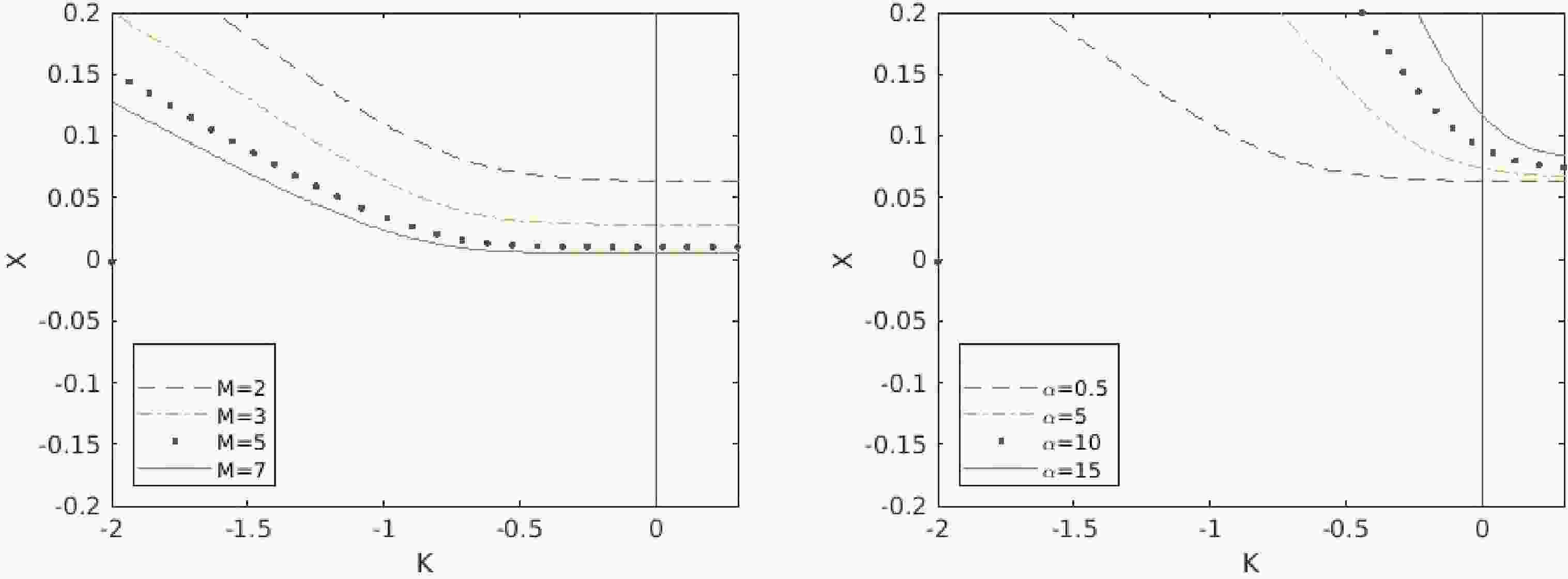
$ X_{0} $ , which is an indication of the formation of naked singularity (NS). Figure 1 (a) reveals the dependence of$ X_{0} $ on the equation of state (23) parameter (κ) for particular values of the massive gravity parameter$ {\mathbb{M}}(=2,3,5,7) $ with fixed$ \phi_{v0}^{2} $ . Also, from this figure, we see that with increasing$ \mathbb{M} $ the tendency of formation of an NS decreases. Therefore, we can say that the addition of graviton mass to this system with the specific choice of rainbow functions (77) deforms the dynamics of the system. In Fig. 1(b), we obtain the$ \kappa-X_{0} $ trajectories by varying the values of$ \alpha(=0.5,5,10,15) $ . In this figure, we see that, with greater values of$ {\alpha} $ , the tendency to form an NS is greater.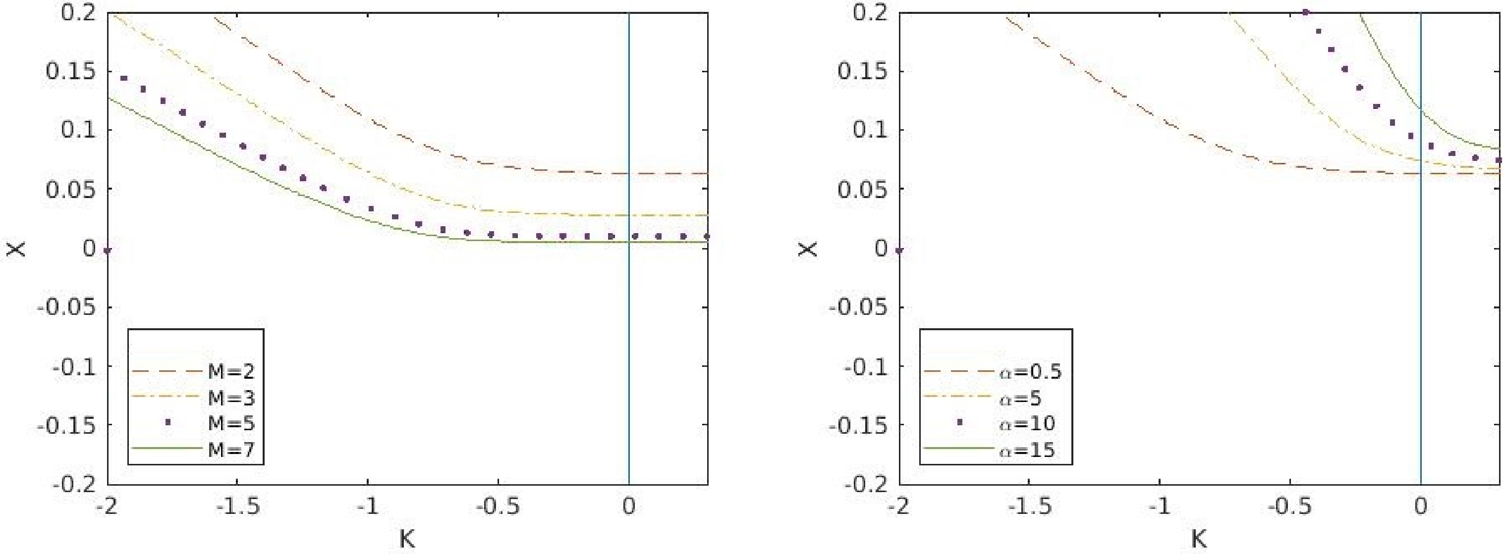
Figure 1. (color online) Figs. (a) and (b) show the variation of
$ X_{0} $ with κ for different values of$ \mathbb{M} $ and α respectively (in Fig. (a), M is equal to$ \mathbb{M} $ ) with$ \phi_{v0}^{2}=0.7 $ ,$ E_{p}=1.221\times 10^{19} $ , and$ E_{1}=1.42\times 10^{-13} $ . In Fig. (a), the initial conditions are$ \alpha=0.5 $ ,$ \beta=2 $ ,$ c=2 $ , and$ c_{2}=2 $ , whereas in Fig. (b), the initial conditions are$ \mathbb{M}=2 $ ,$ \beta=2 $ ,$ c=2 $ , and$ c_{2}=2 $ .In Fig. 2(a), we observe how c affects the collapsing scenario. It is clear that for a greater value of
$ c(=2,3,5,10) $ , the tendency to form NS is lower. In Fig. 2(b), we can observe the effect of$ c_{2} $ on the collapsing system. Similar to that for c, we see that an increase in$ c_{2} $ decreases the possibility of NS.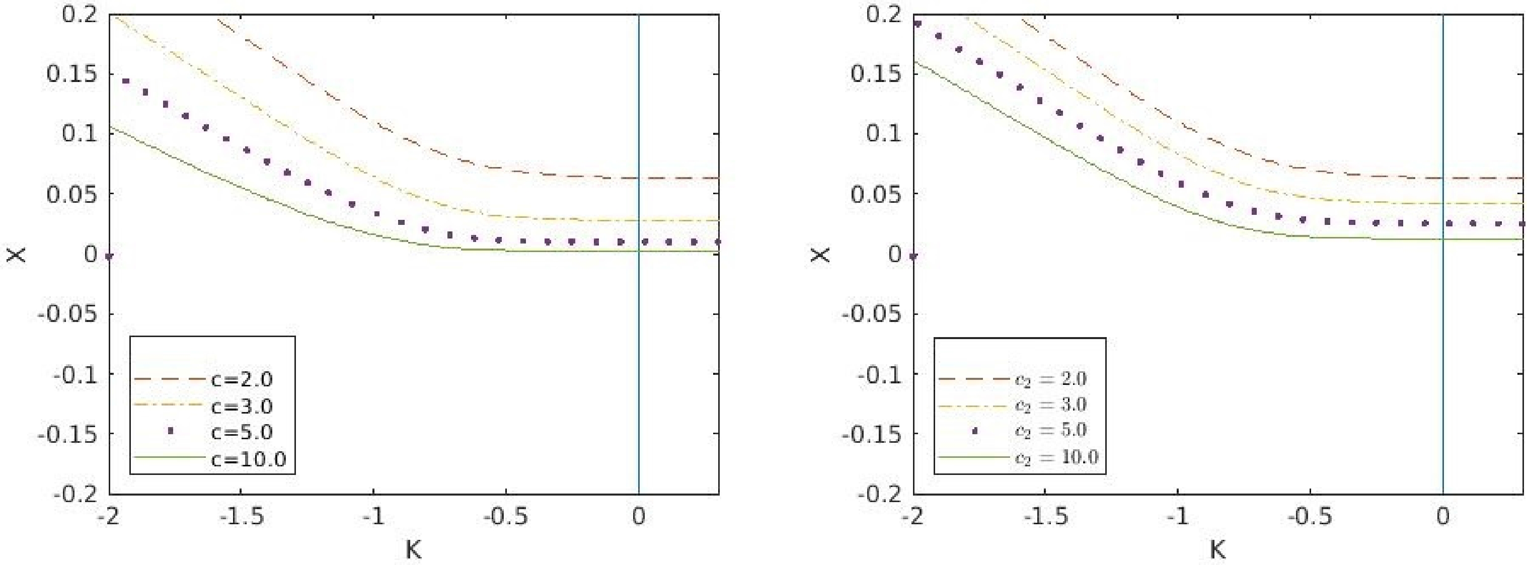
Figure 2. (color online) Figs. (a) and (b) show the variation of
$ X_{0} $ with$ {\kappa} $ for different values of c and$ c_{2} $ , respectively, with$ \phi_{v0}^{2}=0.7 $ ,$ E_{p}=1.221\times 10^{19} $ , and$ E_{1}=1.42\times 10^{-13} $ . In Fig. (a), the initial conditions are$ \mathbb{M}=2 $ ,$ \alpha=0.5 $ ,$ \beta=2 $ , and$ c_{2}=2 $ , whereas in Fig. (b), the initial conditions are$ \mathbb{M}=2 $ ,$ \alpha=0.5 $ ,$ \beta=2 $ , and$ c=2 $ .In Fig. 3, we have showed the effect of the kinetic energy (
$ \phi_{v0}^{2} $ ) of the k-essence scalar field on the collapsing scenario. It has been observed that all values of$ \phi_{v0}^{2} $ predict the same trajectories for the system and form the NS of the collapsing system. Here, we consider the restriction of$ \phi_{v0}^{2} $ not exceeding unity.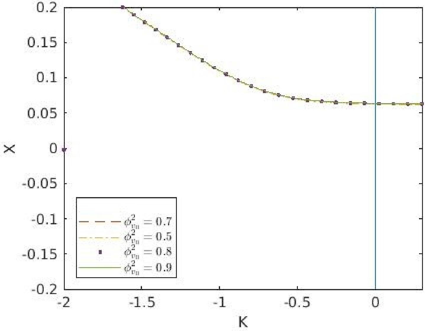
Figure 3. (color online) Variation of
$ X_{0} $ with κ for different values of$ \phi_{v0}^{2} $ with$ E_{p}=1.221\times 10^{19} $ and$ E_{1}=1.42\times 10^{-13} $ and the initial conditions are$ \alpha=0.5 $ ,$ \beta=2.0 $ ,$ c=2.0 $ ,$ c2=2.0 $ and$\mathbb{M}=2.0.$ All the above observations and the corresponding discussions of the
$ \kappa-X_{0} $ trajectories make it clear that the trajectories reside in the positive$ X_{0} $ region, which assures the formation of a naked singularity from the collapse of this system. -
Taking the recommendation of [15, 63, 69, 115–117], we can conclude that a singularity
$ (r=v={\lambda}=0) $ would be strong if the following condition is satisfied$ \begin{equation} \lim\limits_{{\lambda}\to 0}{\lambda}^{2}\psi=\lim\limits_{{\lambda}\to 0}{\lambda}^{2}\bar{R}_{\mu\nu}K^{\mu}K^{\nu}>0, \end{equation} $

(83) where
$ \bar{R}_{\mu\nu} $ is the Ricci tensor and$ \psi=\bar{R}_{\mu\nu}K^{\mu}K^{\nu} $ is defined as a scalar of the k-essence emergent Vaidya massive gravity rainbow spacetime. We would like to mention that this scalar ψ is not the k-essence scalar field and is not coupled with the background gravitational metric$ g_{\mu\nu} $ . Stepping into the footsteps of [62, 69], with the conditions of (70), it can be shown that$ \begin{equation} \lim\limits_{{\lambda}\to 0}{\lambda}^{2}\psi={\cal{G}}^{2}({\cal{E}})\Big({\cal{M}}_{v0}\Big)\frac{1}{4}X_{0}^{2}>0. \end{equation} $

(84) So far we have seen that, if this condition is satisfied for some real and positive roots of
$ X_{0} $ , the naked singularity of the k-essence emergent Vaidya massive gravity rainbow spacetime is strong. In contrast, if there is no positive real root of$ X_{o} $ , we can conclude that no outgoing future directed null geodesics from the singularity exist, i.e., the collapse ends in a black hole.Now from the definition of
$ f_{1}(v) $ and$ f_{2}(v) $ and from (35), we have$ \begin{equation} {\cal{M}}_{v}=\frac{2{\kappa}{\alpha}}{1-2{\kappa}}\Big(\frac{v}{r}\Big)^{2{\kappa}-1}+{\beta}+2r{\cal{F}}^{2}({\cal{E}})\phi_{v}\phi_{vv}. \end{equation} $

(85) Thus, we have
$ \begin{equation} {\cal{M}}_{v0}=\frac{2{\kappa}{\alpha}}{1-2{\kappa}}X_{0}^{2{\kappa}-1}+{\beta}\equiv m_{v0}. \end{equation} $

(86) In the above three cases, i.e.,
$ {\kappa}=0 $ ,$ {\kappa}=1 $ , and$ {\kappa}=-1/2 $ , we have derived the positive roots of$ X_{0} $ for the respective conditions. Also, from Eq. (86), we observe the following situations for the above three cases:(i)
$ {\kappa}=0 $ and${ \cal{M}}_{v0}={\beta} $ , which is positive for any positive value of$ {\beta} $ ,(ii)
$ {\kappa}=1 $ and$ {\cal{M}}_{v0}={\alpha} X_{0}+{\beta} $ , where the positivity of${ \cal{M}}_{v0} $ implies that$ {\alpha} X_{0}+{\beta}>0 $ and(iii)
$ {\kappa}=-1/2 $ and$ {\cal{M}}_{v0}={\beta}-\frac{{\alpha}}{2X_{0}^{2}} $ , where the positive value of${ \cal{M}}_{v0} $ implies that$ 2{\beta} X_{0}^{2}>{\alpha} $ .With the above conditions and the specific rainbow functions (77), we see that
$ \lim\limits_{{\lambda}\to 0}{\lambda}^{2}\psi>0 $ . Therefore, it can be concluded that the naked singularity is strong under the above conditions. -
The authors in [67, 68] described the dynamical horizon (DH) on the basis of [118–122] in the context of k-essence geometry considering the Schwarzschild metric as the background metric. In contrast, in [62, 69], the authors described the apparent horizon (AH) for the generalized Vaidya type geometry. The AH is nothing but the boundary of the trapped surface region in the given spacetime (34). The casual behavior of the trapped surfaces developed in the spacetime during the collapse evolution decides the occurrence of a naked singularity or black hole.
We should remember that the AHs are not invariant properties of a spacetime and are distinct from event horizons (EHs). Within an AH, light does not move away from it. This is in contrast with the EH, where, in a dynamical spacetime, outgoing light rays exterior to an AH (but still interior to the EH) can exist. Specifically, an AH is a local notion of the boundary of a spacetime, whereas an EH is the global notion of a black hole.
-
The AH for the k-essence emergent Vaidya spacetime in massive gravity rainbow (34) can be represented as
$ \begin{eqnarray} \frac{{\cal{M}}(v,r)}{r}=1\Rightarrow \frac{m(v,r)}{r}+{\cal{F}}^{2}({\cal{E}})\phi_{v}^{2}=1, \end{eqnarray} $

(87) with
$ {\cal{F}}({\cal{E}})\neq 0 $ .Considering Refs. [62, 69], the slope of the AH at the central singularity (
$ r\rightarrow 0, v\rightarrow 0 $ ) can be written as$ \begin{eqnarray} \Bigg(\frac{{\rm d}v}{{\rm d}r}\Bigg)_{AH}=\frac{1-m_{r0}-{\cal{F}}^{2}({\cal{E}})\phi_{v0}^{2}}{m_{v0}}=\frac{1+{\mathbb{M}}^{2}c_{2}c^{2}-{\cal{F}}^{2}({\cal{E}})\phi_{v0}^{2}}{\dot{f}_{20}(v)}, \end{eqnarray} $

(88) where we have used Eq. (72).
Now, the sufficient conditions for the existence of a locally naked singularity for the collapsing k-essence emergent Vaidya spacetime in massive gravity's rainbow have been attained. The emergent mass function
$ {\cal{M}}(v,r) $ obeys all the energy conditions and constraints mentioned in (50), (51), and (52). Also, as in [69], there exists an open set of parameter values for which the singularity is locally naked for the case of k-essence emergent Vaidya spacetime in massive gravity's rainbow.It is important not to forget that the k-essence emergent Vaidya spacetime in the massive gravity rainbow metric may exchange radiation with the surroundings, but the mass function (35) cannot totally evaporate due the presence of the massive gravity terms and the kinetic part of the k-essence scalar field, which is a function of v. As an example, in [68], the authors showed the decreasing nature of the black hole mass
$ m(v,r) $ in the k-essence emergent Schwarzschild Vaidya spacetime, but it does not completely vanish by using the DH equation as$ \phi_{v}^{2}\rightarrow 0^{+} $ . -
This paper shows the construction of a theory of the k-essence Vaidya spacetime in massive gravity’s rainbow. We have also analyzed the energy dependent deformation of massive gravity in our work. We have used the Vainshtein mechanism and the dRGT mechanism in the construction of massive gravity in which deformation by the rainbow functions has been considered. This paper also includes an analysis of the gravitational collapse of null fluids in the radiating k-essence Vaidya black hole solution of massive gravity’s rainbow based on the Dirac-Born-Infeld Lagrangian. The above said exploration has been presented in the context of the cosmic censorship hypothesis with the k-essence emergent Vaidya massive gravity rainbow mass function. The Einstein tensor and the energy conditions for the combination of Type-I and Type-II matter field energy-momentum tensor for the k-essence emergent Vaidya massive gravity rainbow spacetime have also been studied thoroughly. We have shed some light on the classification of non-spacelike geodesic for the k-essence emergent Vaidya massive gravity rainbow spacetime which connects the naked singularity in the past, which is a strong curvature singularity in the stronger sense. The central singularity is a node, which allows outgoing non-spacelike geodesics to come out of the singularity pursuing a definite value of the tangent. This positivity of the tangent implies the violation of the strong cosmic censorship conjecture, i.e., the singularity is locally naked, though not necessarily a weak one.
If somehow the value of the tangent does not have a positive value, the central singularity deviates from being a naked one because, in that case, there are no outgoing future-directed null geodesics coming out from the singularity, i.e., the collapse will always lead to a black hole. With these results we have also studied the effects of the graviton mass, the kinetic energy of the k-essence scalar field and the rainbow deformation for a time-dependent system.
We have obtained the contours for the tangent
$ X_{0} $ against the barometric parameter$ {\kappa} $ for different values of other parameters, namely$ {\mathbb{M}} $ ,$ {\alpha} $ ,$ {\beta} $ ,$ \phi_{v0}^{2} $ , etc. Various regimes of the fluid content of the universe such as the radiation ($ {\kappa} > 0 $ ), pressure-less dust ($ {\kappa} = 0 $ ), dark energy ($ {\kappa} < 0 $ ) have been plotted. From those figures it is clear that the negative region contains no trajectories for specific choices of the rainbow functions. This outcome makes us believe the existence of black holes cannot be possible as the end state of collapse in the context of massive gravity's rainbow with the considered parameters.It should be noted that, here, we have studied the structure of the gravitational collapse of a non-rotating type spacetime. The violation of CCC allows us to achieve a naked singularity which by definition is not bounded by any EH. In contrast, there have been considered several models in which the non-spacelike geodesics originate in the central singularity. However, this is not a proof for the nakedness of the singularity. In [123], for the rotating case there should be a consideration of the ergosphere in describing the motion of the non-spacelike geodesics. The authors have also studied in detail the geodesics in the ergosphere of a rotating black hole which has negative energies. An ergoshpere is basically a region located outside a rotating black hole's outer EH. Particularly in non-extremal Kerr spacetime (
$ a < M $ case), a non-spacelike geodesic for particles having negative, zero and positive energy can originate at the central singularity, when the collapse is a black hole. In [124] the authors studied the dynamics of high energy particles, which have negative and positive energies in the vicinity of black holes. They also studied the time of movement of particles with negative energy in the ergosphere. Vertogradov [125] examined the nature of the geodesics for particles with negative energy in Kerr’s metric. Also, we would like to mention that in our article we have not discussed the formation of the ergosphere. We may try to explore this type of formation in the near future.In this study, we found a significant similarity between the k-essence emergent gravity metric and the generalized Vaidya massive gravity metric with the rainbow deformations. Obviously, this may establish another motivation or foundation for gravity's rainbow theory. The result continues to include that the rainbow deformations of the k-essence emergent Vaidya massive gravity metric also satisfy the required energy conditions. Therefore, from a purely physical background, the results are viable and demand for some observational clues on the possibility of observing the naked singularity. The crucial issue then becomes the following: How can the naked singularity be experimentally tested? Let us elaborate this point a bit based on the available literature as follows:
(i) The authors of [126] investigated the optical appearance of a geometrically thin and optically thick accretion disk around the strongly naked Janis-Newman-Winicour (JNW) singularity in their study. Their solution represents an example of a compact object spacetime, which possesses no photon sphere. They [ 126] also established a general observational signature for distinguishable compact objects possessing no photon sphere from black holes.
(ii) In [127, 128], the authors studied the distinction between black holes and naked singularities using the images of their accretion disks. They considered a simplified model of spherical accretion onto the central object and studied the shadows and images of Joshi-Malafarina-Narayan (JMN) [129, 130] for naked singularities.
(iii) Bhattacharya et al. [131] studied a new class of naked singularities and their observational signatures on the basis of suitable junction conditions matched with an expanding FLRW metric with a generic contracting solution of Einstein’s equations on a spacelike hypersurface. They also studied some observational aspects of the resulting two-parameter family of static naked singularity backgrounds.
(iv) Kovacs et al. [132] noted the properties of the accretion disk and observationally different black holes from naked singularities. They considered a rotating solution of the Einstein-massless scalar field equations for the naked singularity, which reduces to the Kerr solution when the scalar charge tends to 1. They also showed their interest in studying the motions of the particles in the gravitational potential of this solution. Depending on the values of the mass, scalar charge, and spin parameter, there are two types of disks that can exist around naked singularities. The first type comprises marginally stable orbits, located outside the naked singularity, while the second type is reachable for the particles and in direct contact with the singularity.
(v) Ortiz et al. [133] studied the observational differences between black holes and naked singularities through the redshift function. They stated that the photons propagating from past to future null infinity through the center of a cloud obtain a frequency shift, which can be measured by distant stationary observers and that it can help in discriminating naked singularities from black holes. They showed that, according to their model, it is possible to differentiate between the formation of a naked singularity and the formation of a black hole based on the detection of photons traversing a collapsing object.
(vi) Vertogradov [134, 135] proposed a method for studying the formation of an eternal naked singularity in the case of gravitational collapse of generalized Vaidya spacetime. Also, in [136, 137], the authors studied the naked singularity using gravitational lensing.
We would like to end our discussion by mentioning that we have analytically discussed the formation of a naked singularity in the k-essence Vaidya spacetime in massive gravity's rainbow. From the above observational discussions of the existence of naked singularity, one may conclude that it is also possible for this type of singularity to exist in reality; however, this needs observational confirmation and evidence.
Data availability: Our manuscript has no associated data.
-
The authors would like to thank the referee for illuminating suggestions on improving the paper. SR is thankful to the Inter-University Centre for Astronomy and Astrophysics (IUCAA), Pune, India, for providing a Visiting Associateship under which a part of this work was carried out.
Collapsing scenario for the k-essence emergent generalized Vaidya spacetime in the context of massive gravity's rainbow
- Received Date: 2022-05-14
- Available Online: 2022-12-15
Abstract: In this study, we investigate the collapsing scenario for the k-essence emergent Vaidya spacetime in the context of massive gravity's rainbow. For this study, we consider that the background metric is Vaidya spacetime in massive gravity's rainbow. We show that the k-essence emergent gravity metric closely resembles the new type of generalized Vaidya massive gravity metric with the rainbow deformations for null fluid collapse, where we consider the k-essence scalar field as a function solely of the advanced or the retarded time. The k-essence emergent Vaidya massive gravity rainbow mass function is also different. This new type k-essence emergent Vaidya massive gravity rainbow metric satisfies the required energy conditions. The existence of a locally naked central singularity and the strength and strongness of the singularities for the rainbow deformations of the k-essence emergent Vaidya massive gravity metric are the interesting outcomes of the present work.


 DownLoad: