


 Abstract
 HTML
HTML Reference
 Related
 PDF
PDF


-
The W mass measurement recently published by the CDF II experiment [1] reports 7 sigma deviation from its standard model (SM) expectation (obtained from an electroweak global fit) and is also in tension with other experimental determinations [2]. The new CDF-II result, the SM expectation from the electroweak fit, and the previous PDG world-average value are as follows [1, 2]:
$ \begin{aligned}[b] m_W^{\rm{CDF-II}}=&80433.5\pm 9.4\; {\rm{MeV}}\,, \\ m_W^{\rm{SM}}=&80357\pm 6\; {\rm{MeV}}\,, \\ m_W^{\rm{PDG}}=& 80379 \pm 12\; {\rm{MeV}} \,. \end{aligned} $

The standard model of particle physics is a precise and concise theory. The fact that we are testing it from many different angles enables us to understand where new physics may arise. This new CDF II W mass measurement, being the most precise one so far, is certainly a remarkable achievement, and the result itself calls for new explorations in particle physics. In this paper, we study and discuss various possibilities of the physics behind such discrepancies in the measurements.
Notably, this new determination of
$ m_W $ took advantage of the large integrated luminosity, kinematics of proton-antiproton collision, and high energy resolution level without an exceedingly large pile-up. Through a template fit to the underlying W boson mass, the measurement was robustly checked against various experimental effects. The result is impressively precise. Several outstanding theories and experimental directions can make the results and interpretation more robust. This measurement is in tension with other experimental measurements from different collaborations [2–6], which calls for comparative studies. An understanding of the various experimental assumptions and calibrations is crucial. In particular, the W boson production and decays are subject to various high order QCD and QED effects, both fixed order and resummed. The differential rate itself has sizable scale uncertainties, resulting from the missing higher-order calculations. It would be useful to understand the theoretical uncertainties behind these "templates" used by the CDF-II experiment. Only with a sufficiently precise theoretical control can the measured W-boson mass be interpreted as a well-defined quantity to be compared with the predictions from the SM and new physics.With the caveat that further experimental and theoretical works are needed to fully establish this discrepancy in W mass determination, these intriguing results call for evaluations of possible new physics sources. Should they come from new physics, plausible BSM scenarios and testable aspects are presented in this work. We discuss the overall picture of electroweak precision observables (EWPO) fit and how several simple, representative models would be able to help improve the fitting. A brief summary is outlined below. Ultimately, a new global average of the W-mass measurements that includes the new CDF-II result should be obtained and used in the global analyses. The combination of W-mass measurements is, however, highly nontrivial given the sizable amount of tension between the CDF-II measurement and previous measurements. In our study, we focus on the comparison between the previous world-average
$ m_W $ measurement and the new CDF-II one rather than their combination.This paper is organized as follows. In Sec. II, we present three types of electroweak (EW) global fits in an effective-field-theory framework, namely the S-T, S-T-
$ \delta G_F $ , and eight-parameter flavor-universal one. Each of them is distinct in terms of correlations, best-fit values, and the amount of tensions between the EW and this new$ m_W $ determination. In Sec. III, we introduce three classes of models, each accompanied with two scenarios, and we verify whether they can help reduce the tension between the SM EW fit and this new direct$ m_W $ measurement. The models we studied include gauge extensions of the SM with new gauge bosons, vector-like top partners, and top squarks. These results are summarized in Table 1. We further check these intuitive models' theory and experimental constraints and comment on their future perspectives. Finally in Sec. IV, we conclude this study.Specifications/models d.o.f. $ \chi^2 $ 

References pre CDF-II $ m_W^{\rm combine} $ 

$ m_W^{\rm CDF-II} $ 

EW fit SM (3) 31 62 76 Sec. II S-T (3)+2 28 30 33 S-T- $ \delta G_F $ 

(3)+3 28 28 28 Universal EW (3)+8 17 17 17 BSM Models $ Z^\prime $ /

$ W^\prime $ (

$ \Delta S=0.1 $ )a

(3)+1b 29 (28) 38 (33) 34 (31) Sec. III A VLQ Top I ( $ \Delta S=0.1 $ )

(3)+2c 29 (29) 34 (32) 38 (34) Sec. III B VLQ Top II ( $ \Delta S=0.1 $ )

(3)+2 28 (53) 33 (31) 37 (33) Sec. III B Top Squark (3)+2d 28 31 34 Sec. III C a $ \Delta S=0.1 $ in the bracket represents the case in which an extra contribution to the oblique parameter S is included, and the corresponding best fit

$ \chi^2 $ s are listed in the parathensis. b While the model has more free parameters, with the gauge symmetry breaking assumption, only one linear combination of parameters enters the fit. c In the simplified singlet and doublet top partner models, there are only two free parameters,

$ M_{T} $ (

$ M_{Q_T} $ ) and

$ \lambda_{T} $ (

$ \lambda_{Q_T} $ ). d In the degenerate soft-mass scenario, only two degrees of freedom of top squarks,

$ m_{\tilde t} $ and

$ \tan\beta $ , are present. In the non-degenerate soft-mass scenarios, three degrees of freedom,

$ m_{\tilde Q_3} $ ,

$ m_{\tilde U_3} $ , and

$ \tan\beta $ , are present. In both scenarios,

$ \tan\beta $ does not change the quality of the fit in a sizable way.

Table 1. Summary of various SM and BSM considerations in this study with the corresponding references. The best fit
$ \chi^2 $ s are listed for various scenarios considered in this study.$ m^{\rm combine}_W $ denotes the new world-average of$ m_W $ from Ref. [7]. For BSM considerations, the best fit values of individual models are presented. However, other direct experimental searches need to be taken into account and these details are discussed in the text. -
Here we provide the interpretation of a shifted
$ m_W $ from an effective-field-theory point of view. We work in the framework of the standard model effective field theory [8, 9]. We choose the$ \{ \alpha,\, m_{Z}, G_{F}\} $ input scheme so that the measurement of$ m_W $ provides a constraint on the operator coefficients. More specifically, we fix the measured values of these input parameters to be as follows [2]:$ \begin{aligned}[b] &\alpha=1/127.940,\,\; \; \; \; m_{Z}=91.1876\, {\mathrm {GeV}}, \,\\& G_{F}=1.1663787\times 10^{-5}\, {\mathrm{GeV}} \,. \end{aligned} $

(1) Thus, any new physics effects that contribute to the measurement of these parameters change the "inferred SM value" and contribute indirectly to the observables. For instance, the 4-fermion operator
$ {\cal{O}}^{1221}_{\ell\ell} = (\bar{\ell}_1 \gamma^\mu \ell_2) (\bar{\ell_2} \gamma_\mu \ell_1) $ contributes to the muon decay process and generates a shift in the inferred SM$ G_F $ (VEV①), which we will later denote as$ \delta G_F $ . We focus on the Z and W pole measurements in our analysis, which are$ \begin{equation} \Gamma_Z \,, \quad \sigma_{\rm{had}} \,, \quad R_{f} \,, \quad A^{0,\, f}_{\rm{FB}} \,, \quad A_{f} \,, \quad A^{\rm{pol}}_{e/\tau} \,, \end{equation} $

(2) where
$ f=e,u,\tau,b,c $ and$ A^{\rm{pol}}_{e/\tau} $ are$ A_e $ and$ A_\tau $ measured from tau polarization measurements at LEP, and$ \begin{equation} m_W \,, \quad \Gamma_W \,, \quad {\rm{BR}}(W\to e\nu) \,, \quad {\rm{BR}}(W\to \mu\nu) \,, \quad {\rm{BR}}(W\to \tau\nu) \,. \end{equation} $

(3) For the Z-pole measurements, we use the results in Ref. [10], where the correlations (if available) are also included. The measurements of the W branching ratios are taken from Ref. [11]. For
$ \Gamma_W $ , we use the PDG result [2]. For$ m_W $ , we consider three scenarios, the "old" world average from PDG [2], the new CDF-II measurement [1] alone, and the "new avg." scenario using the new world-average$ m_W $ from Ref. [7], with$ m_W=80413.3 \pm 8.0 $ MeV, which includes the new CDF-II measurement as well as the LHCb one [6].The SMEFT parameterization in our analysis follows closely those in Refs. [12, 13] (see also Refs. [14–18]), where the contributions to observables from the dimension-6 operators are calculated at the tree-level, but are normalized to the SM predictions. The SM predictions are taken from the central values of the SM-fit in Ref. [19], except for
$ m_W $ , which is taken from Ref. [2]. To account for the parametric and theoretical uncertainties that are absent in this simple treatment, we combine in quadrature the experimental uncertainty of$ m_W $ with that from the "SM EW fits" [2], treating the latter as an effective total "theory" error. This theory error, 6 MeV, mainly comes from the missing higher-order calculations and the parametric uncertainties of input parameters, which include$ m_t $ and$ m_H $ , that enter at the one-loop level. Our results from this simple treatment for the$ S,\,T $ parameters are in good agreement with those from Ref. [19].Before doing a detailed analysis, it is intuitive to first try to understand what kind of new physics contribution can generate a significant shift in
$ m_W $ without modifying any other electroweak observable, as the latter is generally in good agreement with the SM predictions [10]. It is convenient to work on a basis where the operators associated with the W, Y parameters [20] are exchanged for the 4-fermion operators. In this case, the modification of$ m_W $ from dimension-6 operators is given by$ \begin{equation} \delta m_W = \frac{1}{2 c_{2w}} \left[ c^2_w \, \hat{T} - s^2_w \left( \delta G_F + 2 \hat{S} \right) \right] \,, \end{equation} $

(4) where
$ m_W = m_W^{\rm{SM}}(1+\delta m_W) $ ,$ G_F = G_F^{\rm{SM}}(1+\delta G_F) $ ,②$s^2_w \equiv \sin^2\theta_W$ ,$ c^2_w \equiv \cos^2\theta_W $ ,$ c_{2w} \equiv \cos2\theta_W $ , and$ \theta_W $ is the weak-mixing angle. The parameters$ \hat{S} $ and$ \hat{T} $ [20] are related to the S and T parameters [21] by$ \begin{equation} \hat{S} = \frac{\alpha}{4 s^2_w} S \,, \quad \hat{T} = \alpha T \,. \end{equation} $

(5) Note also that the U parameter is generated by dimension-8 operators and is not considered here. Among the three parameters
$ \hat{S} $ ,$ \hat{T} $ , and$ \delta G_F $ , only two independent combinations contribute to the Z-pole observables, which are$ \hat{T}-\delta G_F $ and$ \hat{S} $ , respectively. Therefore, to generate a positive$ \delta m_W $ without changing the Z-pole observables, one needs to keep$ \hat{S}=0 $ and shift$ \hat{T} $ and$ \delta G_F $ simultaneously such that$ \hat{T} = \delta G_F $ . A positive$ \hat{T} $ (and$ \delta G_F $ ) is needed for a positive$ \delta m_W $ .To verify this statement, we first perform a global fit of the three parameters above. The results are presented in Fig. 1. The "old" scenario (cyan), with the world-average
$ m_W $ measurement, is compared with the "new CDF" scenario (magenta), with$ m_W $ from only the new CDF-II measurement, and the "new avg." scenario (gray) using the new world-average$ m_W $ [7]. For easy comparison, we switch to the original (no hat) version of S and T. The left panel shows the 90% confidence level (CL) contour in the S-T plane. For each scenario, two contours are shown: the solid one is from a 2-parameter fit of S and T, setting$ \delta G_F =0 $ , while the dashed one is from the 3-parameter fit (marginalized over$ G_F $ ). For the 3-parameter fits, the contours are also projected on the$ (\delta G_F,\,T) $ plane shown on the right panel. The results are also listed in Table 2.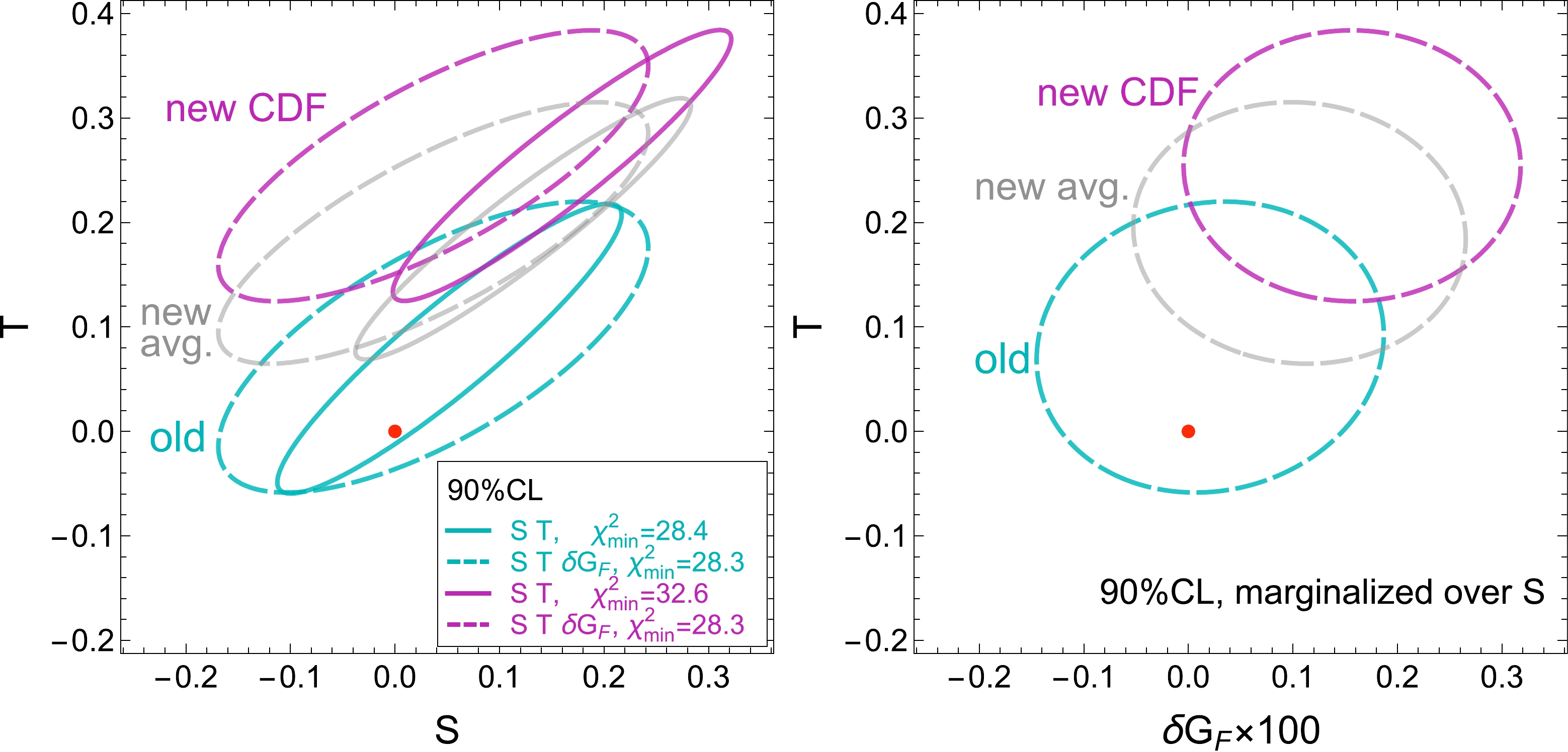
Figure 1. (color online) Results from a 2-parameter fit of S and T (solid contours) and a 3-parameter fit of S, T, and
$ \delta G_F $ (dashed contours) to the current EW precision measurements. The "old" scenario (cyan) uses the current PDG world-average$ m_W $ measurement, the "new CDF" scenario (magenta) uses the new CDF measurement alone for$ m_W $ , and the "new avg." scenario (gray) uses the new world-average$ m_W $ result in Ref. [7], which includes the new CDF measurement. We fix$ U=0 $ as it is generated by dimension-8 operators. The left (right) panel shows the results in the S-T ($ \delta G_F $ -T) plane. The scale for$ \delta G_F $ is amplified by 100 for convenience. All contours correspond to a 90% confidence level (CL).old (PDG) new CDF new avg. 2-para fit $ 1\sigma $ bound

correlation matrix $ 1\sigma $ bound

correlation matrix $ 1\sigma $ bound

correlation matrix S T S T S T S $ 0.052 \pm 0.077 $ 

1 0.92 $ 0.160\pm 0.075 $ 

1 0.93 $ 0.123\pm 0.075 $ 

1 0.94 T $ 0.079 \pm 0.065 $ 

1 $ 0.255 \pm 0.060 $ 

1 $ 0.194 \pm 0.058 $ 

1 3-para fit $ 1\sigma $ bound

correlation matrix $ 1\sigma $ bound

correlation matrix $ 1\sigma $ bound

correlation matrix S T $ \delta G_F $ 

S T $ \delta G_F $ 

S T $ \delta G_F $ 

S $ 0.037 \pm 0.096 $ 

1 0.68 −0.60 $ 0.037\pm 0.096 $ 

1 0.74 −0.62 $ 0.037\pm 0.096 $ 

1 0.76 −0.63 T $ 0.081 \pm 0.065 $ 

1 0.08 $ 0.254 \pm 0.060 $ 

1 -0.002 $ 0.190 \pm 0.058 $ 

1 -0.05 $ \delta G_F $ 

$ (2.1 \pm 7.7)\times 10^{-4} $ 

1 $ (15.7 \pm 7.5)\times 10^{-4} $ 

1 $ (10.6 \pm 7.4)\times 10^{-4} $ 

1 Table 2. Results from the
$ (S,T) $ 2-parameter fit and$ (S,T,\delta G_F) $ 3-parameter fit as in Fig. 1 . One-sigma bounds are quoted here.From Fig. 1, we can see that, indeed, the shift of the central values in the
$ (S,T,\delta G_F) $ 3-parameter fit is consistent with our observation above. From the old$ m_W $ to the new CDF one, the central values of T and$ \delta G_F $ both shift in the positive direction, while the central value of S does not change. We also note that the minimum$ \chi^2 $ values are the same for the old and new scenarios in this case. Meanwhile, for the$ (S,T) $ 2-parameter fit, shifts of both S and T in the positive direction are required to go from the old$ m_W $ measurement to the new CDF one. The minimum$ \chi^2 $ is also increased by approximately 4, suggesting that the$ S,T $ -only scenario exhibits some tension with the new CDF measurement. The "new avg." scenario exhibits a similar pattern but with central values somewhere between the old and new CDF ones, as expected.Let us now move to a more general framework with a complete basis of 8 operators for the Z and W pole observables, assuming flavor universality. The corresponding Lagrangian is given by
$ \begin{aligned}[b] {\cal{L}} =& \frac{c_{WB}}{ m^2_W} {\cal{O}}_{WB} + \frac{c_T}{v^2} {\cal{O}}_{T} + \frac{c^{1221}_{ll}}{v^2} {\cal{O}}^{1221}_{\ell\ell} + \frac{c'_{Hq}}{v^2} {\cal{O}}'_{Hq} \\&+ \underset{f=e,q,u,d}{\sum} \frac{c_{Hf}}{v^2} {\cal{O}}_{Hf} \,, \end{aligned} $

(6) where the operators are listed in Table 3, and
$ v\simeq 246 $ GeV. Note that we keep the flavor labels on the 4-fermion operator$ {\cal{O}}^{1221}_{\ell\ell} $ . This is because the flavor diagonal ones (with indices$ iijj $ ), which can for instance be generated by flavor-preserving interactions with a$ Z' $ -boson, do not contribute to the muon decay (and$ \delta G_F $ ). This information is somewhat unclear under the flavor universality condition, as the$ {\cal{O}}^{ijji}_{\ell\ell} $ operator can be expressed as a combination of flavor diagonal operators using the Fiertz identity. We also choose the convention for$ {\cal{O}}_{WB} $ to have$ c_{WB} = \hat{S} $ (which is different from the convention in, e.g., Ref. [22]). This basis matches the SILH' basis in Refs. [23, 24] with the replacement$ c_{WB} \to c_W + c_B $ . The operator coefficients$ c_{WB} $ ,$ c_T $ , and$ c^{1221}_{\ell\ell} $ have one-to-one correspondences with S, T, and$ \delta G_F $ , given by$ \mathcal{O}_{WB} = \frac{1}{4} gg' H^\dagger \sigma^a H W^a_{\mu\nu} B^{\mu\nu} $ 

$ \mathcal{O}_{T} = \frac{1}{2}(H^\dagger \overleftrightarrow{D_\mu} H)^2 $ 

$ \mathcal{O}^{1221}_{\ell\ell} = (\bar{\ell}_1 \gamma^\mu \ell_2) (\bar{\ell}_2 \gamma_\mu \ell_1) $ 

$ \mathcal{O}_{He} = (i H^\dagger \overleftrightarrow{D_\mu} H )(\bar{e} \gamma^\mu e ) $ 

$ \mathcal{O}_{Hq} = (i H^\dagger \overleftrightarrow{D_\mu} H )(\bar{q} \gamma^\mu q ) $ 

$ \mathcal{O}_{Hu} = (i H^\dagger \overleftrightarrow{D_\mu} H)( \bar{u} \gamma^\mu u ) $ 

$ \mathcal{O}'_{Hq} = (i H^\dagger \sigma^a \overleftrightarrow{D_\mu} H)( \bar{q} \sigma^a \gamma^\mu q) $ 

$ \mathcal{O}_{Hd} = (i H^\dagger \overleftrightarrow{D_\mu} H)( \bar{d} \gamma^\mu d ) $ 

Table 3. A complete operator basis for the Z and W pole observables assuming flavor universality. We keep the flavor labels on
$ \mathcal{O}^{1221}_{\ell\ell} $ to distinguish it from the flavor-diagonal ones ($ iijj $ ), which do not contribute to muon decay. q, l are left-handed$S U(2)_L$ doublets, and e, u, d are$S U(2)_L$ singlets. Note that the convention of$ \mathcal{O}_{WB} $ is slightly different from that in [22].$ \begin{equation} c_{WB} = \hat{S} = \frac{\alpha}{4 s^2_w} S \,, \quad c_T = \hat{T} = \alpha T\,, \quad c^{1221}_{\ell\ell} = -2 \delta G_F \,, \end{equation} $

(7) and the 3-parameter fit can be recovered by simply setting all other operator coefficients to zero.
The
$ 1\sigma $ bounds from the 8-parameter fit are presented in Fig. 2 and Table 4. Again, a comparison is drawn between the "old" scenario (with the PDG world-average$ m_W $ ) and the "new CDF" and "new avg." ones. For the "old" scenario, our results are in good agreements with those in Ref. [12] for the SILH' basis. Caution must be taken in the interpretation of the global fit results, as the introduction of many parameters could result in an over-fitting to the data. As in Ref. [12], here the central values of$ c_{WB} $ and$ C_T $ become negative, and we observe very strong correlations among$ c_{WB} $ ,$ c_T $ , and$ c_{He} $ in the range$ 0.93 $ -$ 0.96 $ (see Table 4), which are also strongly correlated with$ c^{1221}_{\ell\ell} $ . The minimum$ \chi^2 $ in this case is$ 17.1 $ , much smaller than that of the 3-parameter fit ($ 28.3 $ ), suggesting a significant shift in the global minimum. We note also that$ c_{Hd} $ exhibits a significant deviation from the SM due to the measurement discrepancy in the$ A^b_{\rm{FB}} $ measurement of approximately$ 2.5\sigma $ [10, 19].③ However, for the comparison between the "old" and "new CDF" scenarios, we still observe a pattern similar to the case of the 3-parameter fit, where only significant shifts in$ c_T $ and$ c^{1221}_{\ell\ell} $ are needed to accommodate the shift in$ m_W $ . We also note that the 7σ deviation in the CDF$ m_W $ measurement is significantly diluted in the 8-parameter fit. This is expected, as the marginalized bounds become weaker with more parameters. This is also reflected in the strong correlations among$ c_{WB} $ ,$ c_T $ ,$ c_{He} $ , and$ c^{1221}_{\ell\ell} $ , as mentioned above. The situation is different for$ c_{Hd} $ , which is almost in the same direction as$ A^b_{\rm{FB}} $ (or$ A_b $ ) [26], and basically inherited its$ 2.5\sigma $ deviation.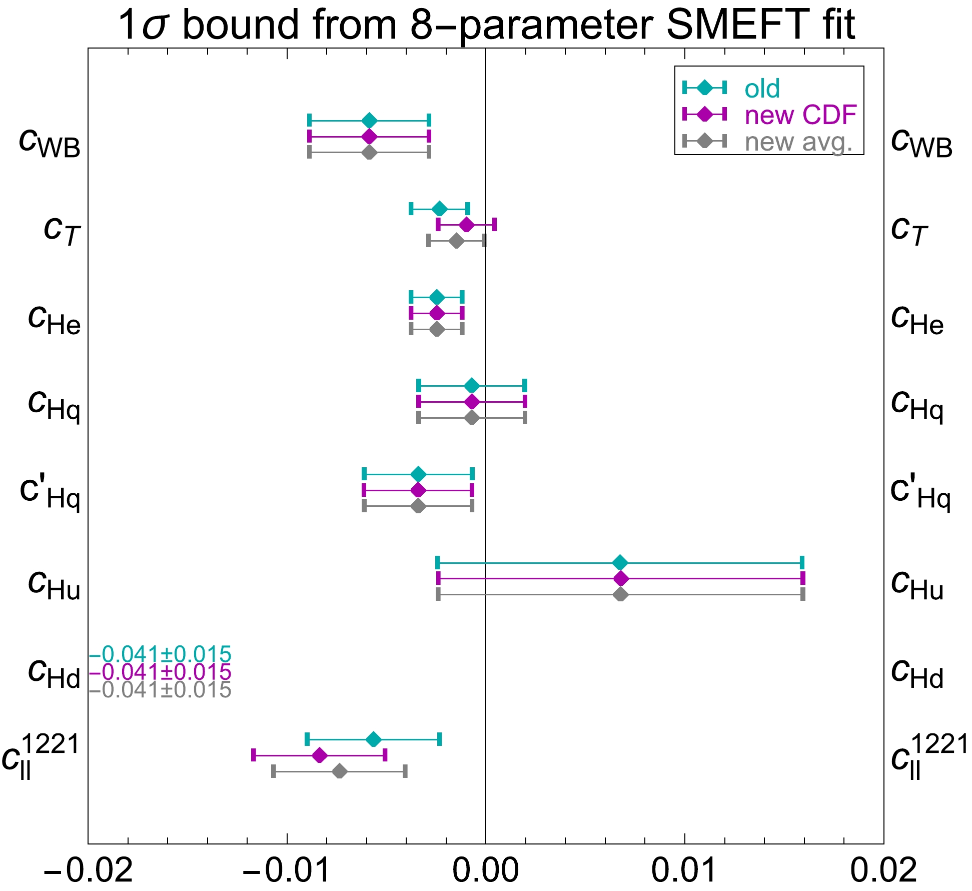
Figure 2. (color online) One-sigma bounds from the 8-parameter SMEFT fit with the operator coefficients listed in Equation 6 and Table 3. The "old" scenario (cyan) uses the current PDG world-average
$ m_W $ measurement, the "new CDF" scenario (magenta) uses the new CDF measurement alone for$ m_W $ , and the "new avg." scenario (gray) uses the new world-average$ m_W $ result in Ref. [7]. Note that$ c_{Hd} $ is out of the plot range owing to the$ A^{b}_{\rm FB} $ measurement at LEP. Its bounds are directly quoted in numbers.$ 1\sigma $ bounds (in %)

correlation matrix old new CDF new avg. $ c_{WB} $ 

$ c_T $ 

$ c_{He} $ 

$ c_{Hq} $ 

$ c'_{Hq} $ 

$ c_{Hu} $ 

$ c_{Hd} $ 

$ c^{1221}_{\ell\ell} $ 

$ c_{WB} $ 

$ -0.59 \pm 0.30 $ 

$ -0.59 \pm 0.30 $ 

$ -0.59 \pm 0.30 $ 

1 0.96 (0.97) 0.96 −0.091 −0.25 −0.16 0.11 0.91 $ c_T $ 

$ -0.23 \pm 0.14 $ 

$ -0.10 \pm 0.14 $ 

$ -0.15 \pm 0.14 $ 

1 0.93(0.94) −0.07 −0.20 −0.16 0.15 0.78 (0.81) $ c_{He} $ 

$ -0.25 \pm 0.13 $ 

$ -0.25 \pm 0.13 $ 

$ -0.25 \pm 0.13 $ 

1 −0.12 −0.29 −0.14 0.05 0.85 $ c_{Hq} $ 

$ -0.07 \pm 0.27 $ 

$ -0.07 \pm 0.27 $ 

$ -0.07 \pm 0.27 $ 

1 −0.30 0.60 0.38 −0.13 $ c'_{Hq} $ 

$ -0.34 \pm 0.27 $ 

$ -0.34 \pm 0.27 $ 

$ -0.34 \pm 0.27 $ 

1 −0.69 0.58 −0.33 $ c_{Hu} $ 

$ 0.67 \pm 0.92 $ 

$ 0.68 \pm 0.92 $ 

$ 0.68 \pm 0.92 $ 

1 −0.07 −0.11 $ c_{Hd} $ 

$ -4.1 \pm 1.5 $ 

$ -4.1 \pm 1.5 $ 

$ -4.1 \pm 1.5 $ 

1 −0.02 $ c^{1221}_{\ell\ell} $ 

$ -0.56 \pm 0.33 $ 

$ -0.84 \pm 0.33 $ 

$ -0.74 \pm 0.33 $ 

1 Table 4. One-sigma bounds from 8-parameter SMEFT fit (shown in Fig. 2 ) and correlation matrix. The one-sigma bounds are shown in percentages (a factor of
$ 10^{-2} $ should be applied to all the bounds). For the correlation matrix, most entries are the same for the three scenarios. The numbers in the parentheses indicate that the new CDF or average values are different from the old results by$ > 0.01 $ . -
This section explores the compatibility of various representative BSM models that help explain this discrepancy.
-
We first focus on the simple models with gauge symmetry
$S U(2) \times S U(2) \times U(1)$ and discuss the low energy consequences of different symmetry breaking patterns. Those models can be seen as the prototype of some more sophisticated models to explain the origin of mass.Case I: left-handed breaking
The first case is that a gauge symmetry of
$S U(2)_1 \times S U(2)_2 \times U(1)_Y$ ($ U(1)_Y $ is the hypercharge gauge symmetry) and a bifundamental scalar Δ neutral under hypercharge can get a VEV to break$S U(2)_1 \times S U(2)_2$ into the diagonal subgroup$S U(2)_L$ , which is identified as electroweak gauge symmetry,$ \begin{eqnarray} \langle \Delta \rangle =\frac{1}{\sqrt{2}}\left(\begin{array}{cc} v_\Delta & 0 \\ 0 & v_\Delta \end{array}\right). \end{eqnarray} $

(8) We can find that two gauge boson triplet
$ W_1^a $ and$ W_2^a $ will mix, and the mass eigenstate$ W^{\prime a} $ and SM gauge triplet$ W^a $ can be obtained through the following rotation matrix:$ \begin{eqnarray} \left(\begin{array}{c} W^a \\ W^{\prime a} \end{array}\right) =\left(\begin{array}{cc} \cos \theta & \sin \theta \\ -\sin \theta & \cos \theta \end{array}\right)\left(\begin{array}{c} W_1^a \\ W_2^a \end{array}\right), \end{eqnarray} $

(9) where the mixing angle is
$ \sin \theta =g_1/\sqrt{g_1^2 +g_2^2} $ . The mass of the$ W^{\prime a} \equiv (W^{\prime +}, Z^\prime, W^{\prime -}) $ triplet is$ \begin{eqnarray} m_{Z^\prime} = m_{W^\prime} = \frac{1}{2}\sqrt{g_1^2 +g_2^2} \,\, v_\Delta. \end{eqnarray} $

(10) We can introduce a
$S U(2)_1$ scalar doublet H, which can be identified as the SM Higgs doublet, to break the electroweak (EW) gauge symmetry. The quantum number under$S U(2)_1 \times S U(2)_2 \times U(1)_Y$ of SM fermions can be assigned as follows:$ \begin{aligned}[b]& L_L \in (2,1,-1/2) \quad L_R \in (1,1,-1), Q_L \in (2,1,+1/6) \\& U_R \in (1,1,+2/3) \quad D_R \in (1,1,-1/3), \end{aligned} $

(11) where
$ L_{L,R} $ can be identified as an SM lepton doublet and singlet, and$ Q_L $ ,$ U_R $ , and$ D_R $ are a quark doublet, up quark, and down quark, respectively (here we neglect the QCD$S U(3)_c$ gauge symmetry). With the above quantum number assignment, we can find that the couplings of$ W^\prime $ to the SM currents are universal and can be written as$ \begin{aligned}[b] {\cal{L}}=&-g \tan \theta W^{\prime a}_\mu \Big( \bar{L}_L \gamma^\mu T^a L_L + \bar{Q}_L \gamma^\mu T^a Q_L\\& +( i H^\dagger T^a (D_\mu H) - i (D_\mu H)^\dagger T^a H) \Big), \end{aligned} $

(12) where g is the EW
$S U(2)_L$ gauge coupling$ g =g_1 \cos \theta $ ,$ T^a =\dfrac{1}{2} \sigma^a $ , and$ \sigma^a $ is Pauli sigma matrices. Then, we can integrate out the massive$ W^\prime $ triplet at the tree level and obtain the effective Lagrangian,$ \begin{aligned}[b] {\cal{L}}_{eff} =&-\frac{g^2 \tan^2 \theta }{2m_{W^{\prime}}^2} J^a_\mu J^a_\mu\,, \\ J^a_\mu =& \bar{L}_L \gamma^\mu T^a L_L + \bar{Q}_L \gamma^\mu T^a Q_L +( i H^\dagger T^a (D_\mu H)+ {\rm h.c.}). \end{aligned} $

(13) We can easily find that there is no correction to the T parameter because there is custodial symmetry in this model. The effective Lagrangian can be expanded in terms of the Han and Skiba operator bases [27] that contribute to EW precision measurements,
$ \begin{eqnarray} {\cal{L}}_{eff} = a^\prime ( O_{l^il^j}^t +O_{l^iq^j}^t + O_{hl^j}^t +O_{h q^j}^t ) + \cdots \,, \quad a^\prime =-\frac{g^2 \tan^2 \theta }{2m_{W^{\prime}}^2 }, \end{eqnarray} $

(14) where the subscripts
$ i,j $ represent the SM fermion generation. Using the universal electroweak fit defined in Sec. II, our results show that this model tends to make the fit even worse, which is easy to understand from Eq. (4), where the additional$ W' $ contributions to$ \delta G_F $ would reduce the W mass.Case II: right-handed breaking
In this section, we consider the model with gauge symmetry
$S U(2)_L \times S U(2)_R \times U(1)_X$ . The$S U(2)_R \times U(1)_X$ is broken into hypercharge symmetry$ U(1)_Y $ at some high scale. Then, the electroweak symmetry$S U(2)_L \times U(1)_Y$ is broken by the Higgs doublet [28]. In this model, the hypercharge is defined as$ \begin{eqnarray} Y=T_R^3+X. \end{eqnarray} $

(15) Here, we suppose that
$S U(2)_R \times U(1)_X$ is broken by a$S U(2)_R$ triplet with$ U(1)_X $ charge$ X=1 $ [29, 30],$ \begin{eqnarray} \Delta =\frac{1}{\sqrt{2}}\left(\begin{array}{cc} \Delta^+/\sqrt{2} & \Delta^{++} \\ \Delta^{0} & -\Delta^+/\sqrt{2} \end{array}\right). \end{eqnarray} $

(16) The neutral component gets a VEV
$ \langle \Delta^{0} \rangle = v_R $ and breaks the$S U(2)_R$ guage symmetry. The gauge bosons will get the mass,$ \begin{eqnarray} m_{W_R^\pm}^2=\frac{1}{4} g_R^2 v_R^2\,, \quad m_{Z_R}^2 =\frac{1}{2} (g_R^2 +g_X^2) v_R^2. \end{eqnarray} $

(17) At some low energy scale, the
$S U(2)_L$ Higgs doublet H with$ U(1)_X $ charge$ X=1/2 $ gets the VEV$\langle H \rangle =v_{\rm SM}$ to break EW. Then, the neutral gauge bosons will mix, and their mass matrix is given by$ \begin{aligned}[b] \frac{1}{4} \begin{pmatrix} W^{3R}_{\mu} & A^X_{\mu} & W^3_{\mu} \end{pmatrix} \begin{pmatrix} 2 g_R^2 v_R^2 & - 2 g_R g_X v_R^2 & 0 \\ - 2 g_R g_X v_R^2 & g_X^2 (2 v_R^2 + v_{\rm SM}^2) & -g_X g_L v_{\rm SM}^2 \\ 0 & -g_X g v_{\rm SM}^2 & 2g^2 v_{\rm SM}^2 \end{pmatrix} \begin{pmatrix} W^{3R}_{\mu} \\ A^X_{\mu} \\ W^3_{\mu} \end{pmatrix} \ . \end{aligned} $ 
(18) We suppose that the EW scale is much smaller than the
$S U(2)_R$ breaking scale; therefore, we have a small parameter$\epsilon = v_{\rm SM}^2/v_R^2 \ll 1$ . The mass matrix can be diagonalized by rotation matrix R,$ \begin{eqnarray} \begin{pmatrix} W^{3R}_{\mu} \\ A^X_{\mu} \\ W^3_{\mu} \cr \end{pmatrix} = {{{\boldsymbol R}^\dagger }} \begin{pmatrix} A_\mu \cr Z_\mu \cr Z^\prime_\mu \cr \end{pmatrix} \, \end{eqnarray} $

(19) where A, Z, and
$ Z^\prime $ denote the mass eigenstates. The eigenstate A is the photon, Z is identified with the SM Z boson, while$ Z^\prime $ is the heavy neutral gauge boson. The couplings of this model are related to the electric charge by$ \begin{eqnarray} g_R = \frac{e}{\sin \phi \cos \theta_W} \, , \quad g_X = \frac{e}{\cos \phi \cos \theta_W} \, , \quad e = g \sin \theta_W \, , \end{eqnarray} $

(20) where
$ \theta_W $ is the weak mixing angle ($ \epsilon \to 0 $ ) and ϕ is the additional mixing angle ($ \sin \phi \equiv g_X/\sqrt{g_R^2 +g_X^2} $ ). The approximate mass expressions of$ Z_\mu $ and$ Z_\mu ^\prime $ at the linear order of the small parameter$ \epsilon $ are$ \begin{eqnarray} m_Z^2 = \frac12 v_{SM}^2 (g_Y^2+g_L^2 ) \left[1 - \epsilon \sin^4 \phi \right] +{\cal O}(\epsilon^2) \ , \end{eqnarray} $

(21) $ \begin{eqnarray} m_{Z^\prime}^2 = \frac12 v_R^2 (g_R^2+g_X^2 ) \left[1 + \epsilon \sin^4 \phi \right]+ {\cal O}(\epsilon^2) \ , \end{eqnarray} $

(22) where hypercharge coupling can be identified as
$ \begin{eqnarray} \frac{1}{g_Y^2} = \frac1{g_R^2} + \frac1{g_X^2}\ . \end{eqnarray} $

(23) We can see that
$ {g_X^2}/{g_Y^2} = 1 + \tan^2 \phi $ and$ {g_R^2}/{g_Y^2} = 1 + 1/{\tan^2 \phi} $ ; therefore, the perturbativity of$ g_X $ and$ g_R $ requires$ 0.027 <\tan \phi <36 $ . The study presented in [31] investigated a similar model at a low energy effective interaction level.The quantum number of SM fermions under
$S U(2)_L \times S U(2)_R \times U(1)_X$ can be assigned as follows:$ \begin{aligned}[b]& L_L \in (2,1,-1/2) \\& L_R \in (1,1,-1), Q_L \in (2,1,+1/6) \\& U_R \in (1,1,+2/3), \quad D_R \in (1,1,-1/3). \end{aligned} $

(24) In this model, we assume that SM fields do not take the
$S U(2)_R$ charge; therefore, it is similar to the$ 2-1-1 $ model.The mixing matrix R has the following approximate form for small
$ \epsilon $ :$ \begin{aligned}\\[-8pt] {\boldsymbol R} = \left ( \begin{matrix} \sin \phi \cos \theta_W & \cos \phi \cos \theta_W & \sin \theta_W \cr \sin \phi \sin \theta_W + \epsilon \frac{\sin^3 \phi \cos^2 \phi}{\sin \theta_W} & \cos \phi \sin \theta_W - \epsilon \frac{\cos \phi \sin^4 \phi}{\sin \theta_W} & - \cos \theta_W \cr - \cos \phi + \epsilon \cos \phi \sin^4 \phi & \sin \phi + \epsilon \cos^2 \phi \sin^3 \phi & - \epsilon \cot \theta_W \cos \phi \sin^3 \phi \cr \end{matrix} \right )\ , \end{aligned} $ 
(25) and we can simply derive the SM fermion couplings.
The couplings of Z and
$ Z^\prime $ to SM fermion can be written as$ \begin{aligned}[b] g_{Z_\mu f} =& g_X \cos \phi \sin \theta_W Q_X - g \cos \theta_W T_L^3 \\ =& \frac{e}{\sin \theta_W \cos \theta_W} \left( \sin^2 \theta_W Q - T_L^3 -\epsilon \sin^4 \phi Q_X \right) , \end{aligned} $

(26) $ \begin{aligned}[b] g_{Z_\mu^\prime f} =& g_X (\sin \phi + \epsilon \cos^2 \phi \sin^3 \phi)Q_X \\&- g (- \epsilon \cot \theta_W \cos \phi \sin^3 \phi)T_L^3 \\ =& \frac{e}{\cos \theta_W} \left( \frac{\sin \phi}{\cos \phi} Q_X + \frac{ \epsilon \cos \phi \sin^3 \phi}{\sin^2 \theta_W} ( -T_L^3 +Q \sin^2 \theta_W) \right). \end{aligned} $

(27) At the
$S U(2)_L$ unbroken phase$ \epsilon =0 $ , the coupling of$ Z^\prime_\mu $ to the SM fields is only from its mixing with$ U(1)_X $ ; therefore, its coupling is just proportional to$ U(1)_X $ charge$ g_{Z^\prime f} =e Q_X \tan \phi/\cos \theta_W $ . After integrating out$ Z_\mu^\prime $ , the Wilson coefficients of the effective operators will be proportional to$ Q_X^2 $ of the corresponding currents. The effective Lagrangian expanded in terms of the Han and Skiba language bases [27] is given by$ \begin{aligned}[b] {\cal{L}}_{\rm eff} =& \frac{a}{2}\Big(O_h +\frac{1}{2}O_{l^il^j}^s +2O_{e^ie^j}^s +O_{l^ie^j} -\frac{2}{3}O_{l^i u^j} \\&+\frac{1}{3}O_{l^i d^j} -\frac{1}{3}O_{q^i e^j} -\frac{4}{3}O_{e^i u^j} +\frac{2}{3}O_{e^i d^j} \, \\ &-\frac{1}{2}O_{h l^i}^s +\frac{1}{6} O_{h q^i}^s +\frac{2}{3} O_{h u^i}^s -\frac{1}{3} O_{h d^i}^s - O_{h e^i}^s\Big)+\cdots. \end{aligned} $

(28) where
$ a =-e^2 \tan^2 \phi/(m_{Z^\prime}^2 \cos^2 \theta_W) $ , and the subscripts$ i,j $ represent the fermion generation. Because the electroweak precision measurements do not involve four quark operators, we do not explicitly write them out here. We can see that all the four-fermion operators here are from the Y parameter contribution, where the Y parameter is$ \begin{eqnarray} Y = -\frac{a m_W^2}{g_Y^2}. \end{eqnarray} $

(29) Here, Y is defined from the
$ O'_{2B} $ operator coefficient$ -g_Y^2 Y / 2 m_W^2 $ .We can find that the custodial symmetry violation effect is
$ \begin{eqnarray} \frac{a}{2} O_h = - \frac{g_R^2+g_X^2} {2 m_{Z^\prime}^2} \sin^4 \phi |h^\dagger D^\mu h)|^2 \,, \end{eqnarray} $

(30) which is coincident with Z mass shift
$ \Delta m_Z^2 = - \epsilon \sin^4 \phi m_Z^2 $ in Eq. (21). The corresponding T parameter from the tree level gauge boson mixing can be obtained as follows:$ \begin{eqnarray} T = - \frac{a v^2_{SM}}{2\alpha} = \frac{\epsilon \sin^4 \phi}{\alpha}. \end{eqnarray} $

(31) In this simple case, we find that LHC di-muon resonances search [32] excludes the
$ 95\ $ % best-fit parameter space for$ m_{Z^\prime} <5 $ TeV, considering the recent CDF-II results. However,$ Z^\prime $ bounds from LHC searches can be eliminated by introducing some vector-like (VL)$S U(2)_R$ fermion doublets to mix with SM fermions. For example, suppose that a VL lepton$S U(2)_R$ doublet$ L^\prime =(\nu^\prime, e^{\prime-}) $ with X charge$ Q_X =-1/2 $ interacts with the electron doublet and singlet through the Yukawa couplings of some extra scalars. After the neutral components of these scalars get VEVs (suppose that their VEVs are smaller than$ v_R $ ; then, the gauge symmetry breaking pattern does not change),$ e^{\prime -} $ will mix with left- and right-handed electrons, and the mixing angles are supposed to be$ \theta_L $ and$ \theta_R $ . Thus, SM chiral electrons can also interact with$ Z^\prime $ through these mixings, and their coupling$ g_{Z\mu^\prime f } $ in Eq. (27) will change into$ \begin{aligned}[b] g_{Z^\prime e_L} =&\frac{e}{2\cos \theta_W}\Big( \cot(\phi) S_{\theta_L}^2 - \tan (\phi)\Big)\,,\\ g_{Z^\prime e_R} =&\frac{e}{2\cos \theta_W}\Big( \cot(\phi) S_{\theta_R}^2 - \tan (\phi) (1 + C_{\theta_R}^2 ) \Big), \end{aligned} $

(32) where
$ g_{Z^\prime e_{L}} $ ($ g_{Z^\prime e_{R}} $ ) is the coupling of the (right-) left-handed electron to$ Z^\prime $ ,$ S_{\theta_{L,R}} \equiv \sin \theta_{L,R} $ ($ C_{\theta_{L,R}} \equiv \cos \theta_{L,R} $ ), and the overall factor$ 1/2 $ is from the$ Q_X $ charges of electrons and VL lepton$ L^\prime $ . The coupling proportional to$ S_{\theta_{L,R}} $ is from the mixings between$ e_{L,R} $ and$ e^{\prime-} $ . Notice that we neglect the terms proportional to$ \epsilon $ in the above expressions. We can find that there is a cancellation among the terms in$ g_{Z^\prime e_{L,R}} $ ; therefore, the LHC detection bounds on$ Z^\prime $ can be significantly relaxed by tuning the parameters ϕ and mixing angle$ \theta_{L,R} $ . Thus, in this case, there should be plenty of unexcluded parameter space to explain the recent CDF anomaly.Now we can perform the data fit to show the favorite parameter space of the recent CDF-II data. As discussed above, to remove the LHC bounds on
$ Z^\prime $ , we can assume that the couplings of$ Z^\prime $ to SM fermion currents are eliminated by tuning ϕ and mixing angles$ \theta_{L,R} $ for simplicity; therefore, this model only corrects the oblique parameters S and T. We calculate the best-fit band (2 σ around the local minima of the model) in the$ \{\tan \phi, m_{Z^\prime } \} $ plane considering the recent CDF-II data, as shown in Fig. 3. Because the loop corrections can contribute to the S parameter, we also show the data fit with extra$ S=0.1 $ contribution in the right panel (the left panel is for no extra S contribution). In the left panel, because the total$ S=0 $ , the corresponding T parameter is in the range (0.09, 0.18), which agrees with Fig. 1 given that the contributions to the global fits from the remaining operators are eliminated. Meanwhile, in the right panel, because the extra positive S contribution is included, the T parameter lower bound is enhanced, with the data fit preferring the large coupling region.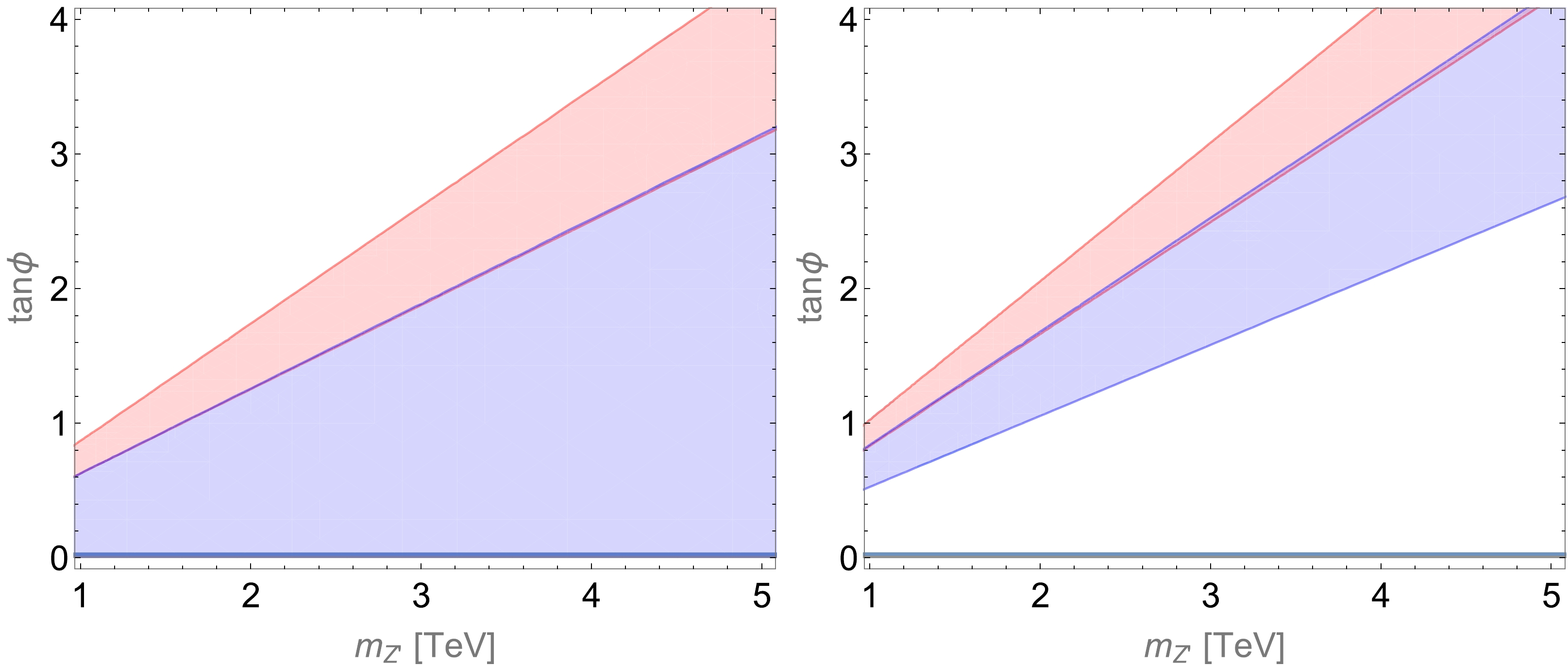
Figure 3. (color online) The red and light blue contours correspond to the
$ 95\ $ % best-fit band with and without the recent CDF-II results. The region below the dark blue line$ \tan\phi < 0.027 $ is not allowed by perturbation requirement. The left and right panels correspond to the extra$ S=0 $ and$ 0.1 $ cases, respectively. -
In the composite Higgs model, vector-like (VL) composite top partners mix with top quarks to generate the top quark mass. In most models, the singlet and doublet top partners always exist. The phenomenology of VL quarks are extensively studied in [33–42]. In the following, we simplify the top partner models to study their phenomenology in general.
Singlet top partner
First, we focus on the VL quark singlet T with hypercharge
$ Y=2/3 $ to mix with the top quark. Its general interactions with the top are given by$ \begin{eqnarray} {\cal{L}}=-y_t \bar{Q}_L H t_R -y_T \bar{Q}_L H^c T_R -M_T \bar{T}T +h.c. \end{eqnarray} $

(33) After Higgs get the VEV, we can obtain the mass of the top and singlet top partner,
$ \begin{aligned}[b] m_t^2 =& \frac{1}{2}\Bigg(M_T^2 +\lambda_t^2 +\lambda_T^2\\& -\sqrt{(M_T^2 +\lambda_T^2 +\lambda_t^2)^2 -4M_T^2\lambda_t^2 }\Bigg)\,, \\ m_T^2 =& M_T^2\left(1+\frac{\lambda_T^2}{M_T^2 -m_t^2} \right)\,, \quad \lambda_i =y_i v_{\rm SM} \ , \end{aligned} $

(34) and then, we obtain the EW precision measurement parameters generated from this extra top partner singlet [43, 44].
After integrating out the singlet top partner, we can obtain the EFT Lagarange in the Han and Skiba bases relevant to EW precision measurements,
$ \begin{aligned}[b] a_h=&-\frac{\alpha}{v_{\rm SM}^2} T\,, \quad a_{WB}=\frac{\alpha}{8 \sin \theta_W \cos \theta_W v_{\rm SM}^2} S\,,\quad \\ a_{HQ}^{(1)} =& \frac{\lambda_{T}^2}{4M_T^2v_{\rm SM}^2} + \frac{\lambda_{T}^2 \lambda_t^2}{16 \pi ^2 M_T^2 v_{\rm SM}^4} \left(1 + \log \frac{\lambda_t^2}{M_T^2} \right) \\& -\frac{\lambda_{T}^4}{256 \pi ^2 M_T^2 v_{\rm SM}^4} \left( 17 + 14 \log \frac{\lambda_t^2}{M_T^2} \right) \,, \\ a_{HQ}^{(3)} =& -\frac{\lambda_{T}^2}{4M_T^2 v_{\rm SM}^2} +\frac{\lambda_{T}^4}{256 \pi^2 M_T^2 v_{\rm SM}^4} \left( 9 + 14\log \frac{\lambda_t^2}{M_T^2} \right) \,, \end{aligned} $

(35) where
$ \begin{aligned}[b] T =& \frac{N_c \lambda_T^2( 2\lambda_t^2 \log (\frac{M_T^2}{\lambda_t^2}) +\lambda_T^2 -2 \lambda_t^2 )}{16 \pi \sin^2 \theta_W m_W^2 M_T^2},\\ S =& \frac{N_c \lambda_T^2( 2 \log (\frac{M_T^2}{\lambda_t^2}) -5)}{18 \pi M_T^2}, \end{aligned} $

(36) $ \{a_h, a_{WB}, a_{HQ}^{(1)},a_{HQ}^{(3)}\} $ are the coefficients of bases$ \{O_h, O_{WB}, O_{hQ}^s, O_{hQ}^t \} $ in [45], where$ O_{hQ}^{s,t} $ are the operators involving the top doublet (because the singlet top partner only interacts with the top doublet), and$ N_c $ is the QCD color number.Similarly, we can obtain the
$ 95 \ $ % best-fit bands in the$ \{M_T, \lambda_{T}/M_T \} $ plane with and without considering the new CDF data (the red and blue regions in Fig. 4). In the right panel, we include the extra contribution of the composite vector partners to the S parameter in the data fit, supposed to be$ S=0.1 $ . In the left-panel, as the new CDF data prefers$ T>0.1 $ (see the solid magenta contour in the left panel in Fig. 1), the red region cannot cover the decouple region$ \lambda_T/M_T \to 0 $ . The perturbation condition requires that$ y_T<\sqrt{4\pi} $ , which excludes the yellow region in Fig. 4. The direct detection of$ 13 $ TeV LHC on the singlet top partner excludes the mass region$ m_T <1.31 $ TeV [46], which corresponds to the black region in Fig. 4. The red and blue dashed lines are the projected exclusion reaches of the$ 14 $ TeV high luminosity LHC (HL-LHC) with luminosity$ {\cal{L}} =3 $ ab$ ^{-1} $ and$ 27 $ TeV high energy LHC (HE-LHC) with luminosity$ {\cal{L}} =15 $ ab$ ^{-1} $ (which corresponds to$ m_T \lesssim 1.8 $ TeV and$ 3.8 $ TeV) [47, 48], respectively. In the right panel, since the extra$ S=0.1 $ contribution to EWPT from the composite vector meson is introduced, the lower bound of the T parameter in Fig. 1 is enhanced, which also enhances the lower bounds of coupling$ \lambda_T /M_T $ from data fit with and without the new CDF data. Because this model does not correct neither the interactions of four light fermions nor the gauge interactions of light fermions, this simple model has a significant unexcluded best-fit parameter space to explain the anomaly in the CDF data. We can also find that, combining with the perturbation condition of Yukawa coupling$ y_T $ , the mass of the VL quark T should be lighter than approximately$ 4.5 $ TeV (3.2 TeV) to explain the new CDF data for the extra$ S=0 $ ($ S=0.1 $ ) case. And the future HE-LHC can almost exclude these two cases (the case with extra$ S=0.1 $ can be fully excluded) if there are no signals of the heavy quark T.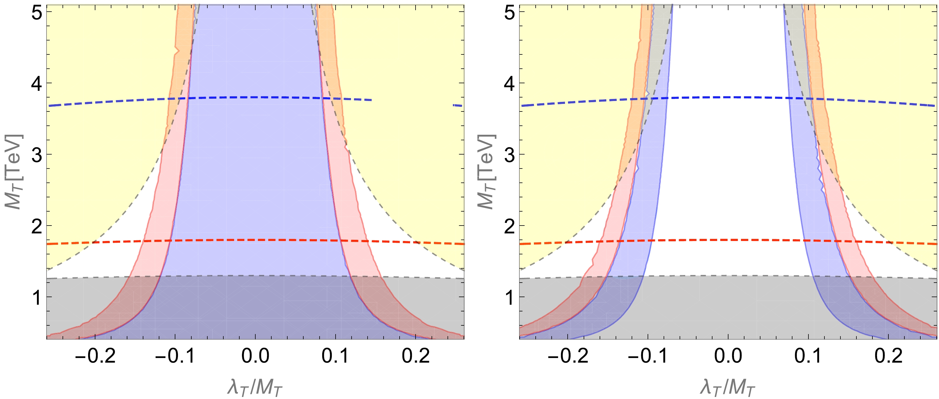
Figure 4. (color online) The red and blue contours correspond to the
$95$ % best-fit bands with and without the most recent CDF results. The light dark region is excluded by LHC direct detection [46]. The red and blue dashed lines are the prospective reaches of HL-LHC and HE-LHC [47, 48]. The yellow region is not allowed by the perturbation condition. In the right panel, the contribution of composite vector partners to the S parameter, supposed to be$ S=0.1 $ , is included.Top partner doublet with
$ Y= 1/6 $ We can also introduce the VL quark doublet
$ Q_T $ with hypercharge$ Y=1/6 $ to mix with the top. Its general interactions are given by$ \begin{eqnarray} {\cal{L}}=-y_t \bar{Q}_L H t_R -y_{Q_T} \bar{Q}_{TL} H^c t_R -M_{Q_T} \bar{Q}_T Q_T +{\rm h.c.} \end{eqnarray} $

(37) The expressions of the top and top partner mass are similar to Eq. (34),
$ \begin{aligned}[b] m_t^2 =& \frac{1}{2}\left(M_{Q_T}^2 +\lambda_t^2 +\lambda_{Q_T}^2 -\sqrt{(M_{Q_T}^2 +\lambda_{Q_T}^2 +\lambda_t^2)^2 -4M_{Q_T}^2\lambda_t^2 }\right)\,, \\ m_{Q_T}^2 =& M_{Q_T}^2\left(1+\frac{\lambda_{Q_T}^2}{M_{Q_T}^2 -m_t^2} \right)\,. \end{aligned} $

(38) The EW precision measurement parameters from the top partner doublet can be expressed as [43, 44]
$ \begin{aligned}[b] a_h=&-\frac{\alpha}{v_{SM}^2} T\,, \quad a_{WB}=\frac{\alpha}{8 \sin \theta_W \cos \theta_W v_{SM}^2} S\,, \\ a_{HQ}^{(1)} =& -\frac{\lambda_t^2 \lambda_{Q_T}^2 }{384 \pi^2 M_{Q_T}^2 v_{SM}^4} \left( 1 + 6\log \frac{\lambda^2_t}{M_{Q_T}^2 v_{SM}^2} \right) \,,\\ a_{HQ}^{(3)} =& -\frac{\lambda_t^2 \lambda_{Q_T}^2 }{96 \pi^2 M_{Q_T}^2 v_{SM}^4}\,, \end{aligned} $

(39) where
$ \begin{aligned}[b] T = \frac{N_c \lambda_{Q_T}^2( 6\lambda_t^2 \log (\frac{M_{Q_T}^2}{\lambda_t^2}) +2\lambda_{Q_T}^2 -9 \lambda_t^2 )}{24 \pi \sin^2 \theta_W m_W^2 M_{Q_T}^2}\,,\end{aligned} $

$ \begin{aligned}[b] S =\frac{N_c \lambda_{Q_T}^2( 4 \log (\frac{M_{Q_T}^2}{\lambda_t^2}) -7)}{18 \pi M_{Q_T}^2}\,. \end{aligned} $

(40) Following the same procedures as above, we show the
$95$ % best-fit bands with and without considering the new CDF data in the red and blue contours in Fig. 5. In the right panel, the extra contribution$ S=0.1 $ from composite vector partners is also included. The light black region corresponds to the excluded region$ M_{Q_T} < 1.37 $ TeV from LHC direct search [46]. The red and blue dashed lines correspond to the projected exclusion reach of HL-LHC with luminosity$ {\cal{L}} =3 $ ab$ ^{-1} $ and HE-LHC with luminosity$ {\cal{L}} =15 $ ab$ ^{-1} $ [47, 48]. The yellow region is not allowed by the perturbation condition of$ y_{Q_T} $ . The physics of this model is almost the same as that in the singlet top partner case, and we will not repeat it. As in the above model, a significant unexcluded best-fit parameter space in this model can explain the new CDF data. Similarly, to explain the anomaly in the CDF data, the mass of Q can not be heavier than$ 5.8 $ TeV (4.4 TeV) for the extra$ S=0 $ ($ S =0.1 $ ). The HE-LHC can almost exclude the case with extra$ S =0.1 $ if the VL quark Q is not found.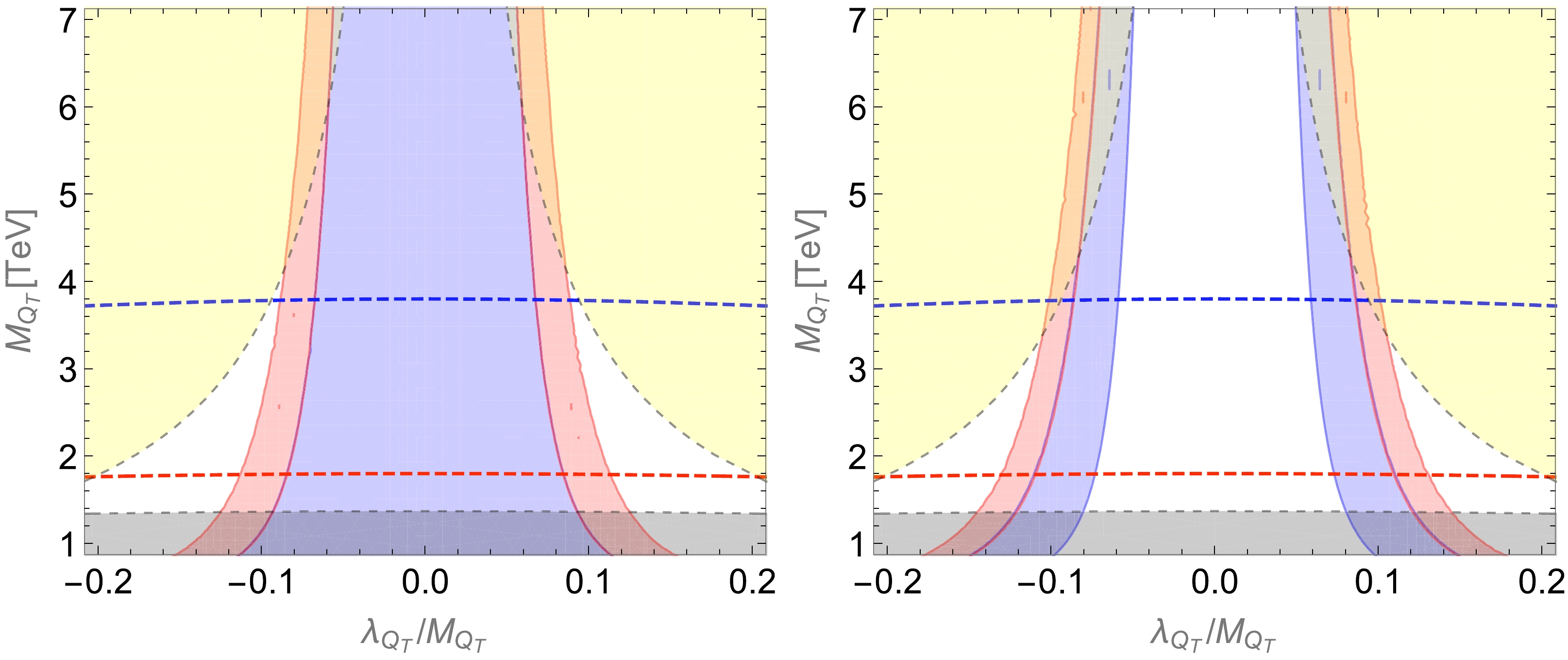
Figure 5. (color online) In these two panels, the red and blue contours correspond to the
$95$ % best-fit band with and without the most recent CDF results. The light dark region is excluded by LHC direct detection [46]. The meanings of the red dashed line, blue dashed line, and yellow region are the same as those in Fig. 4 . In the right figure, the extra contribution$ S=0.1 $ from composite vector partners is included in the data fit. -
The top squark is a representative case for weakly coupled states in the loop that could accommodate the discrepancy. It is instructive and informative to explore the underlying dynamics in this direction. First, we start with a pair of squarks and assume that other electroweak states are decoupled. In R-parity conserving supersymmetry, we would need either a neutralino or a gravitino to serve as the lightest supersymmetric particles. With a bino-like neutralino consistent with the DM direct detection experiments, we can further check the bino contribution to the low energy effective operators. In the context of R-parity violating supersymmetry, we can have the stop being the LSP that can decay promptly or be displaced. These R-parity violating operators are typically sufficiently small so that they would not affect the EWPOs considered here. Regardless of the top squark lifetime, the LHC puts powerful constraints on them. We choose 400 GeV as a minimum requirement on the stop mass [49]. The mass range corresponds to the stop having mass splitting with the LSP around 20 GeV and a shorter lifetime than that coverable by the reach of the typical disappearing track or displaced vertex search. New searches with soft displaced vertices can help improve the constraints further.
The stop sector with the mass matrix
$ (\tilde t_L, \tilde t_R) $ $ \begin{eqnarray} \begin{pmatrix} m_{\tilde Q_3}^2+m_t^2+D_L & m_t X_t \\ m_t X_t & m_{\tilde u_3}^2+m_t^2+D_R \end{pmatrix} \end{eqnarray} $

(41) In the above equation,
$ X_t $ is related to the SUSY parameters$ A_t $ , μ, and$ \tan\beta $ as$ X_t= A_t - \mu \cot \beta $ .$ D_L $ and$ D_R $ are the D-term contributions to top squark masses.Degenerate top-squark soft masses
We begin by considering the degenerate stop soft masses,
$ m_{\tilde Q_3}=m_{U_3}=m_{\tilde t} $ . The mass matrix will yield stop mass eigenstates$ (\tilde t_1, \tilde t_2) $ with mass eigenvalues of$ {m_{\tilde t_1}, m_{\tilde t_2}} $ .At one-loop order, many operators will be generated. Those most constrained are also relevant for our discussion here, in particular for the S-T-
$ \delta G_F $ fit, as [50]$ \begin{aligned}[b] c_T=& \frac {h_t^4} {64\pi^2 m_{\tilde t}^2} \left[\left(1+\frac 1 2 \frac {g^2 c_{2\beta}} {h_t^2}\right)^2-\frac 1 2 \frac {X_t^2} {m_{\tilde t}^2} \left(1+\frac 1 2 \frac {g^2 c_{2\beta}} {h_t^2}\right) +\frac 1 {10} \frac {X_t^4} {m_{\tilde t}^4} \right]\\ c_W=& \frac {h_t^2} {640\pi^2 m_{\tilde t}^2} \frac {X_t^2}{m_{\tilde t}^2},\; \; \; c_B= \frac {h_t^2} {640\pi^2 m_{\tilde t}^2} \frac {X_t^2}{m_{\tilde t}^2}\\ c_{WB}=& -\frac {h_t^2} {384\pi^2 m_{\tilde t}^2} \left[\left(1+\frac 1 2 \frac {g^2 c_{2\beta}} {h_t^2}\right)-\frac 4 5\frac {X_t^2}{m_{\tilde t}^2}\right] \end{aligned} $

$ \begin{aligned}[b] c_{2W}= \frac {g^2}{320 \pi^2 m_{\tilde t}^2},... \end{aligned} $

(42) where
$ c_{2\beta}\equiv \cos(2\beta) $ and$ h_t\equiv y_t \sin\beta $ .④⑤ Here, we omit the details of a few other one-loop generated operators as they have very minor impact on the fit.With the generated operators from the top squark sector, we can put into the S-T parameter fit considered in Sec. II. In Fig. 6, we show the 68% and 95% best-fit regions with and without the new CDF
$ m_W $ mass determination in red and blue contours, respectively. The EW fit without the CDF results allows for large parameter regions filling the spaces across zero. As anticipated, the recent CDF results require larger S and T parameters to restrain the allowed stop parameter space. The best fit region at a 95% level requires the top squark to be as light as 200-400 GeV. The required parameter space would be incompatible with other EWPO and Higgs observables.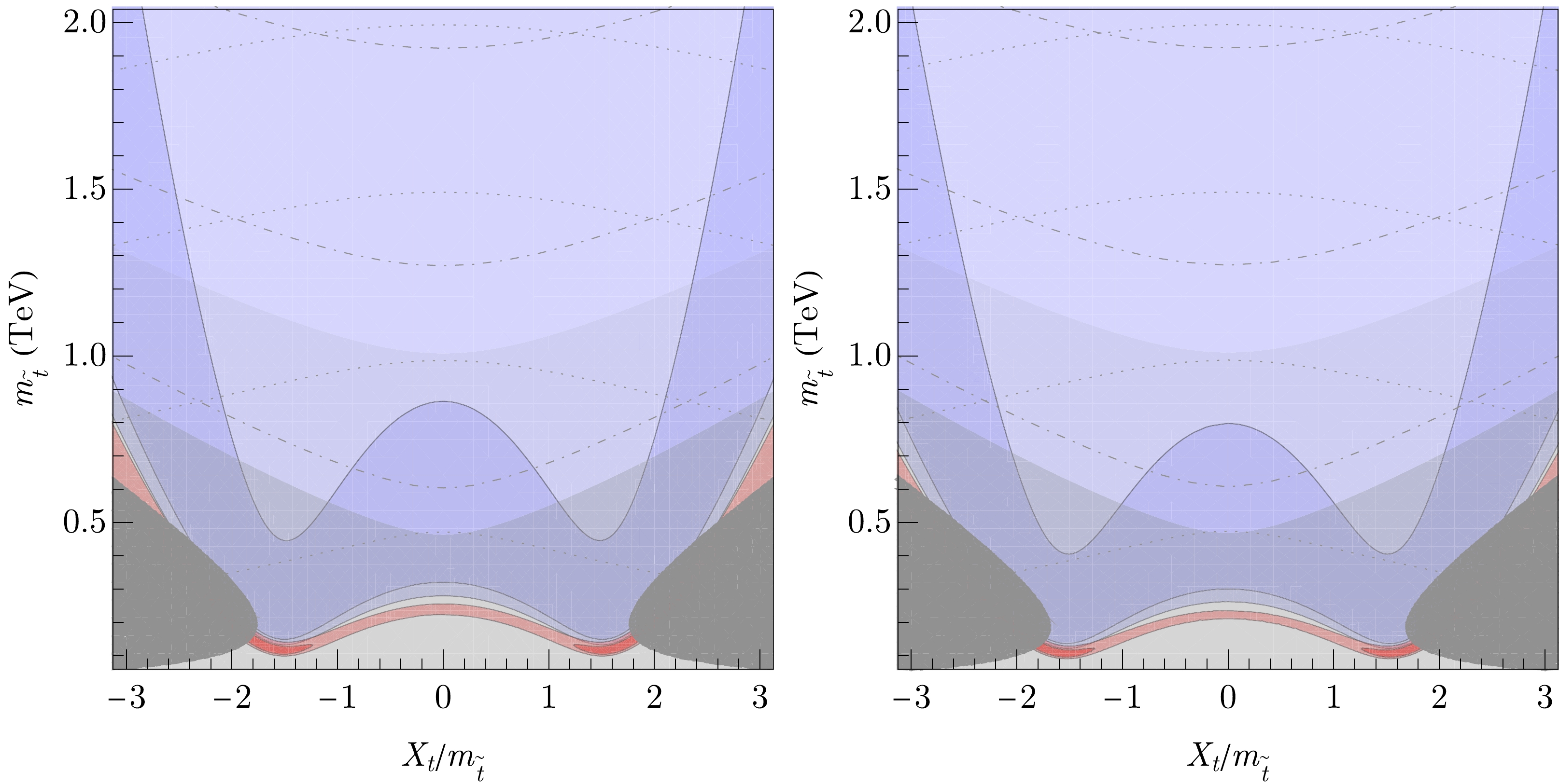
Figure 6. (color online) The 68% and 95% fitted parameter range in the top squark parameter space with degenerate stop soft masses, for
$ \tan\beta=10 $ (left panel) and$ \tan\beta=3 $ (right panel). The recent CDF results require larger S and T parameters to restrain the allowed stop parameter space, as shown in the red regions. The pre-CDFII results are shown in the blue shaded regions. The gray shaded region is color breaking, and hence, it is excluded. The light gray region corresponds to the lighter stop mass of 400 GeV and 800 GeV, representing the current LHC bounds on long-lived stops and prompt stops, respectively. The gray dot-dashed and dotted lines represent the top squark mass eigenstates. More details can be found in the text.The mass scale these solutions point to is so small that one could also worry about the validity of EFT. Further, considering that we conclude the top squark with degenerate soft mass terms to be insufficient for generating the required shift in the oblique parameter, given the current LHC constraints, we can safely discard this possibility.
Still, this provides valuable information to understand the situation with scalar doublets at the loop level. One can consider extending the considerations to multiple specifies, mainly through lepton partners, e.g., light staus [51, 52]. These can be a promising direction to explore.
Non-degenerate top-squark soft masses
From the EFT analysis in Sec. II, we understand that the ability to generate shifts in the S and T parameter directions is crucially important. In particular, from the above discussion, a simple top squark scenario cannot explain the new CDF-II discrepancy between the experimental measurements and the EW fitted W-boson mass. While the top squark sector can already generate custodial symmetry breaking parameters at the one-loop level, one can consider further enhancing these physics effects using the soft mass terms. Non-degenerate top squark soft mass terms will enhance the T parameter. We consider non-degenerate left-handed top squark and right-handed top squark soft mass parameters
$ m_{Q_3} $ and$ m_{U_3} $ .We define the ratio between the top squark soft mass parameters as
$ \begin{equation} rr\equiv \frac {m_{U_3}^2} {m_{Q_3}^2}, \end{equation} $

(43) and then, we can express the particularly relevant Wilson coefficients as follows, using the standard MSSM parameters already introduced earlier:
$ \begin{aligned}[b]\\[-7pt] c_T=& \frac {h_t^4} {16\pi^2 m_{\tilde Q_3}^2} \Bigg[\frac 1 4 \left(1+\frac 1 2 \frac {g^2 c_{2\beta}} {h_t^2}\right)^2+2 \frac {X_t^2} {m_{\tilde Q_3}^2} \left(1+\frac 1 2 \frac {g^2 c_{2\beta}} {h_t^2}\right)\left(-\frac {1-5 rr -2 rr^2} {8(1-rr)^3} +\frac {3 rr^2} {4(1-rr)^4} \log(rr)\right) \\&\left.+ \frac {X_t^4} {m_{\tilde Q_3}^4} \left(\frac {1+10rr+rr^2} {4(1-rr)^4}+\frac {3rr(1+rr)} {2(1-rr)^5} \log(rr)\right)\right]\\ c_W=& \frac {h_t^2} {16\pi^2 m_{\tilde Q_3}^2} \frac {X_t^2}{m_{\tilde Q_3}^2}\left(\frac{1-8rr-17rr^2} {12(1-rr)^4}+\frac {3rr^2+rr^3} {2(1-rr)^5} \log(rr)\right) \\ c_B=& \frac {h_t^2} {16\pi^2 m_{\tilde Q_3}^2} \frac {X_t^2}{m_{\tilde Q_3}^2}\left(\frac{-23-8rr+7rr^2} {12(1-rr)^4}+\frac {-4-12rr+3rr^2+rr^3} {6(1-rr)^5} \log(rr)\right) \\ c_{WB}=& \frac {h_t^2} {16\pi^2 m_{\tilde Q_3}^2} \left[-\frac 1 {24} \left(1+\frac 1 2 \frac {g^2 c_{2\beta}} {h_t^2}\right)+\frac {X_t^2}{m_{\tilde Q_3}^2}\left(\frac {5+33rr-3rr^2+rr^3} {24(1-r)^4}+\frac {2rr + rr^2} {2(1-rr)^5} \log(rr) \right)\right] \end{aligned} $ 
(44) and the full list of generated operators can be found here [53, 54]. In this calculation we decoupled the right-handed bottom squark for simplicity. One can consider adding it and finding better fit to data. Another viewpoint of this loop function can be on the mass basis, where we can consider the non-degenerate top squark masses generating loop-function variations.
To understand the enhancement, we show in Fig. 7 the ratios of Wilson coefficients of various terms as a function of
$ rr $ with respect to the corresponding values of the degenerate case where$ rr=1 $ . For all of$ c_T $ ,$ c_W $ ,$ c_B $ , and$ c_{WB} $ , the non-degenerate soft-mass$ rr $ enters the L-R mixing term proportional to$ X_t^2/m_{Q_3}^2 $ . For$ c_T $ , the non-degenerate soft-mass$ rr $ further enters the L-R doubly mixing term proportional to$ X_t^2/m_{Q_3}^2 $ . We can see in this figure that the non-degenerate soft mass could provide a factor for a few enhancements in these terms. In particular, the contributions to$ c_T $ and$ c_B $ are enhanced, which helps in lifting the S and T directions.
Figure 7. (color online) Ratios of various terms in the Wilson coefficients as a function of the soft mass ratios
$ rr\equiv m_{U_3}^2/m_{Q_3}^2 $ . The reference values with$ rr=1 $ for these five terms$ c_T (X_t^4/m_{Q_3}^4) $ ,$ c_T (X_t^2/m_{Q_3}^2) $ ,$ c_W (X_t^2/m_{Q_3}^2) $ ,$ c_B (X_t^2/m_{Q_3}^2) $ , and$ c_{WB} (X_t^4/m_{Q_3}^2) $ are 1/40, -1/16, 1/40, 1/40, and 1/30, respectively.In Fig. 7, the reference values with
$ rr=1 $ for these five terms$ c_T (X_t^4/m_{Q_3}^4) $ ,$ c_T (X_t^2/m_{Q_3}^2) $ ,$ c_W (X_t^2/m_{Q_3}^2) $ ,$ c_B (X_t^2/m_{Q_3}^2) $ , and$ c_{WB} (X_t^4/m_{Q_3}^2) $ are 1/40, –1/16, 1/40, 1/40, and 1/30, respectively. This ratio is monotonic on$ rr $ and becomes a suppression factor for$ rr>1 $ . Note that this preference implies that the light top squark is preferred to be right-handed, which also makes the top squark parameter space less constrained at the LHC. Another notable feature of these enhancements is their contribution to the S parameter, proportional to$ 4c_{WB}+c_T+c_B $ , and all these terms have the same sign. Further, although the two terms comes with opposite signs for$ c_T $ , the term and enhancement proportional to$ x_T^4/m_{Q_3}^4 $ is dominant in size in the$ X_t/m_{Q_3}\gg 1.6 $ regions. Hence, the inclusion of non-degenerate top squark soft masses with$ rr<1 $ will lead to a better fit to the new$ m_W $ results.We show the top squark parameter space for various values of
$ rr $ in Fig. 8. We adopt a similar convention to that in Fig. 6. We emphasize a few important features here. As before, given that CDF-II$ m_W $ determination is significantly better than others, with the best precision, we compare the results obtained with the CDF-II$ m_W $ alone as the$ m_W $ input with the results reported for$ m_W $ before the CDF-II determination. The 68% and 95% best-fit regions with the CDF-II$ m_W $ are shown in the red shaded regions. As the new$ m_W $ prefers non-zero BSM contributions and is incompatible with the null SM hypothesis, the preferred BSM (red) regions are very restrictive. In contrast, the blue-shaded regions describe the 68% and 95% preferred regions with pre-CDFII$ m_W $ determination. It covers and allows a complete decoupling direction where$ m_{Q_3} $ goes to infinity with$ X_t $ going to zero.
Figure 8. (color online) The 68% and 95% fitted parameter range in the top squark parameter space with non-degenerate stop soft masses. The corresponding top squark parameters are as follows. Top-left panel:
$ rr=0.9 $ ,$ \tan\beta=10 $ ; top-right panel:$ rr=0.9 $ ,$ \tan\beta=3 $ ; bottom-left panel:$ rr=0.8 $ ,$ \tan\beta=10 $ ; bottom-right panel:$ rr=0.6 $ ,$ \tan\beta=10 $ . The blue (red) shaded regions represent the best fit regions with pre-CDFII combined$ m_W $ (CDF-II$ m_W $ alone). The gray shaded region is that with tachyonic light stop mass, and the light gray region corresponds to LHC direct search constraints. The dash-dotted and dotted contours label the top squark mass eigenvalues with a separation between them of 0.5 TeV. The orange lines correspond to two empirical constraints for our metastable electroweak vacuum to tunnel into a color-breaking vacuum (further details are in the text).In Fig. 8, we also use the gray shaded region to represent the color-breaking parameter space and hence disallow solutions there. The light gray region corresponds to a light stop mass of 400 GeV and 800 GeV, respectively, indicating the current LHC bounds on long-lived stops and prompt stops. We also provide dash-dotted and dotted contours to label the top squark mass eigenvalues in units of TeV. The lowest lines of each one represent 0.5 TeV and 1 TeV, respectively. The difference between the contour lines on top squark mass eigenvalues is 0.5 TeV.
We show the results for a few benchmark parameters in the non-degenerate top squark scenarios in this figure. These scenarios are as follows. Top-left panel:
$ rr=0.9 $ ,$ \tan\beta=10 $ ; top-right panel:$ rr=0.9 $ ,$ \tan\beta=3 $ ; bottom-left panel:$ rr=0.8 $ ,$ \tan\beta=10 $ ; bottom-right panel:$ rr=0.6 $ ,$ \tan\beta=10 $ . First of all, the results for the non-degenerate case shown in Fig. 8 are allowed and compatible with the current constraints, in contrast to the case of the degenerate soft-mass results shown in Fig. 6. The newly allowed regions are for$ X_t/m_{Q_3}>1 $ , and are consistent with the enhancements analysis in Eq. 44 and Fig. 7.The results of different
$ rr $ values are comparatively shown in the top-left panel, bottom-left panel, and the bottom-right panel of Fig. 8. We can see that a lower$ rr $ value renders smaller needed$ X_t $ values. Such behavior is a natural result of the enhancement associated with small$ rr $ values. Hence, small$ rr $ values will improve the compatibility with the new CDF-II$ m_W $ measurement. A small$ rr $ value also implies a lighter right-handed top squark for a fixed value of the left-handed top squark soft mass$ m_{Q_3} $ . There, the color-break vacuum constraints and the LHC direct search constraints are stronger, as can be observed in the gray shaded regions. Comparing the top-left panel and top-right panel, we can see the impact of different values of$ \tan\beta $ . The band is dragged more outwards, toward higher$ X_t $ , for a lower$ \tan\beta $ . As$ h_t $ becomes lower for a lower$ \tan\beta $ , one needs a larger$ X_t $ to compensate for the needed operator size.A large
$ X_t $ can generate a new and deeper color-breaking vacuum associated with the scalar direction. We would require our electroweak vacuum to be metastable and have a low zero-temperature tunneling rate longer than the age of our universe. The actual calculation is very complex and depends on many other parameters, and we have empirical and approximated constraints from [55, 56]. Here in Fig. 8, we use the orange dashed curve to represent the empirical constraint from Ref. [55],$ \begin{equation} A_t^2+3\mu^2 < 7.5 (m_{Q_3}^2+m_{U_3}^2). \end{equation} $

(45) When
$ A_t^2\gg \mu^2 $ , one can replace the left-hand side of the above equation with$ X_t^2 $ . Further, Ref. [56] has derived another approximate constraint, and using parameter in this work,$ \begin{equation} A_t^2 \lesssim \left(3.4 (1+rr)+0.5 |1-rr|\right)m_{Q_3}^2+60 m_Z^2. \end{equation} $

(46) Again, when
$ A_t^2\gg \mu^2 $ , one can replace the left-hand side of the above equation with$ X_t^2 $ . We show this constraint in orange dotted lines. We can see that such consideration limits us to smaller$ X_t/m_{Q_3} $ regions, and a detailed tunneling numerical consideration, with additional parameters defined in MSSM, would help establish the best-fit point in the top squark case.Overall, we see that the non-degenerate top squark soft mass parameters fit the new data much better compared to the degenerate case. Interestingly, the preferred stop parameter direction also yields a significant correction to the Higgs mass via large mixing. Although we do not attempt to fit the observed Higgs mass here, it is well-known that the TeV scale top squark with large mixing can fit it. However, other new physics can also contribute to the Higgs mass. Further, although not yet constraining in the majority of the allowed parameter space, the precision Higgs program can start to play more important roles in the scenarios considered in this study.
-
The new W mass determination from the CDF-II experiment is remarkable. Together with many other precision measurements, we stress-test the concise SM. This intriguing result calls for further explorations in many new directions. Experimentally, new measurements in near and future experiments would help fully establish and converge the measured values. Theoretically, differential cross sections matching the experimental templates or improved theoretically-clean determination methods shall be explored. With a joint effort of theory and experiments, the physical meaning of the W mass determination will also be better clarified, especially when the experimental templates are generated through well-defined and uncertainty-evaluated precision theory calculations.
Furthermore, as discussed in this work, the tension between the SM and
$ m_W $ measurements in the EW fit, if fully established, certainly signals the possibility of new physics. We can explore various BSM scenarios behind such discrepancies. Given the sizable difference in the W mass, the new physics scale needs to be not too far above the TeV scale. Moreover, the new physics can be at the electroweak scale if it generates this discrepancy via loops. Direct new physics searches at the LHC and other experiments will reveal or rule out the new physics model candidates. For instance, one can directly search for new gauge bosons, new top partners, etc., at current and future colliders. The electroweak precision program and the Higgs precision program will also further extract the possible imprints of new physics.Finally, the W-mass puzzle can be easily resolved by a
$ WW $ -threshold scan program at future lepton colliders, such as the ILC [57], CEPC [58], and FCC-ee [59], as well as the C3 [60] and muon colliders [61], which will measure$ m_W $ to a precision of approximately or even below 1 MeV. If the discrepancy with the SM is confirmed, such a precise measurement would also point towards a more definite upper bound on the scale of new physics. High energy future colliders [62, 63] will most likely be able to cover the new physics sources generating such discrepancies. -
The authors would like to thank Majid Ekhterachian and Tony Gherghetta for helpful discussions. We particularly thank Tao Han for helpful discussions in various stages of this work.
Note added: Recent studies [7, 64–66] also performed EW global fits to the new CDF
$ m_W $ measurements, which are generally in good agreement with our results.
Speculations on the W-mass measurement at CDF
- Received Date: 2022-06-13
- Available Online: 2022-12-15
Abstract: The W mass determination at the Tevatron CDF experiment reported a deviation from the SM expectation at the 7σ level. We discuss a few possible interpretations and their collider implications. We perform electroweak global fits under various frameworks and assumptions. We consider three types of electroweak global fits in the effective-field-theory framework: the S-T, S-T-


 DownLoad: