Total decay width of ${\boldsymbol{H} \boldsymbol\to \boldsymbol{gg} }$ using the infinite-order scale-setting approach based on intrinsic conformality

In quantum chromodynamics (QCD), the Higgs boson plays an important role in the precision test of the Standard Model (SM), and it is also helpful for searching new physics beyond the SM. The Higgs boson decays into two gluons. This is an important channel for studying the Higgs phenomenology [1]. The coupling of the Higgs to gluons is predominantly mediated by the top quark within the SM, and the high-order QCD corrections to this process can be evaluated by means of an effective theory in which the top quark is integrated out [2]. At present, the perturbative QCD (pQCD) correction to the total decay width of the Higgs decay channel $ H \to gg $, e.g., $ \Gamma(H \to gg) $, is calculated up to next-to-next-to-next-to-next-to-leading order ( $ { \rm N^{4}LO} $) in the limit of a large top-quark mass [3–11]. Therefore, we face the opportunity of achieving precise pQCD prediction on $ \Gamma(H \to gg) $.

It is helpful to reduce the pQCD uncertainties as much as possible. Among them, the error caused by using the conventional scale-setting approach is usually treated as an important systematic error for pQCD prediction. Such an error in making fixed-order prediction occurs because one conventionally assumes an arbitrary renormalization scale to perform the numerical analysis, which is usually chosen as the typical momentum flow of the process, the one assumed to be the effective virtuality of the strong interaction, the one that eliminates large logs to achieve a more convergent series, etc. This ad hoc assignment of renormalization scale causes mismatching of $ \alpha_s $ and the corresponding coefficients. Thus, the coefficients of the QCD running coupling at each order strongly depend on the choice of renormalization scale as well as the renormalization scheme. However, as indicated by the renormalization group invariance, a physical observable must be independent of the choice of renormalization scale. In the literature, the principle of maximum conformality (PMC) [12–15] has been suggested to remove such renormalization scale ambiguity. It is well known that the $ \alpha_s $-running behavior is governed by the renormalization group equation (RGE). Then, the $ \{\beta_i\} $-terms that emerged in the pQCD series can be inversely adopted for fixing the correct $ \alpha_s $-value of a high-energy process. The purpose of PMC is to rightly determine the effective coupling constant of the process (whose argument is called the PMC scale) with the help of the RGE [16, 17], whose prediction is found to be independent of any choice of renormalization scale and satisfies the requirement of renormalization group invariance. The PMC scale-setting procedure agrees with the standard scale-setting procedure of Gell-Mann and Low [18] in the QED Abelian limit (small number of colors, $ N_C \to 0 $ [19]).

Many successful PMC applications have been explored in the literature. Previously, the PMC has been applied for dealing with the decay width $ \Gamma(H\to gg) $ [20–22]. Note that the PMC was originally introduced as a multi-scale approach, in which distinct effective couplings (and hence the PMC scales) at each order were derived because different categories of $ \{\beta_i\} $-terms occur at each order. Furthermore, because the same category of $ \{\beta_i\} $-terms emerges at different orders, the determined PMC scales are in perturbative form. This leads to the fact that the precision of the PMC scales at higher orders decreases with the increment of perturbative orders, given that fewer $ \{\beta_i\} $-terms are known for fixing the value of higher-order $ \alpha_s $. Thus, the PMC multi-scale approach shall have explicit residual scale dependence [23], and if the convergence of the perturbative series of the PMC scale is weak, such residual scale dependence could be large [24].

By further exploiting the intrinsic conformality (iCF) property into PMC, a new infinite-order scale-setting approach, called the PMC$ _\infty $ approach, has been recently proposed in Ref. [25]. The PMC$ _\infty $ approach follows from the PMC, and its resultant conformal coefficients are the same as those of PMC at each perturbative order but sets the effective PMC scales at each order by requiring all the scale-dependent $ \{\beta_i\} $-terms at each order to vanish exactly and separately [25]. Following this approach, the newly fixed PMC scales at each order are in definite form and are no longer in perturbative series. Thus, the residual scale dependence of the previous PMC scales, owing to their previous perturbative nature, can be exactly eliminated. This indicates that the precision of the previous PMC predictions on the total decay width $ \Gamma(H\to gg) $ [20–22] may be further improved by applying the PMC$ _\infty $ approach. It is thus interesting to conduct a detailed study on $ \Gamma(H\to gg) $ by using the PMC$ _\infty $ approach.

Practically, the width of the Higgs decays into two gluons at the $ \alpha_s^6 $-order level can be expressed as

where the Fermi constant $G_{\rm F}=1.16638 \times 10^{-5}\; {\rm{GeV}}^{-2}$, $a_s= \alpha_s/4\pi$, and $ \mu_r $ stands for an arbitrary renormalization scale. The perturbative coefficients $ C_{k\in[0,4]}(\mu_r) $ at the initial scale of $ \mu_r=M_H $ under conventional $ \overline{\rm MS} $-scheme can be read from Refs. [2–11]. As has been argued in Refs. [20–22], it is important to first transform them into those under a physical momentum space subtraction scheme (mMOM-scheme) [26–31] to avoid the ambiguities of fixing the PMC scales with the help of the RGE. The mMOM-scheme is gauge dependent, a detailed discussion of gauge dependence after applying the PMC has been done in Ref. [32], which shows that if the gauge parameter $ \xi\in[-1,1] $, the mMOM prediction will have weaker ξ-dependence. Concerning definiteness, we adopt the Landau gauge ( $ \xi=0 $) to conduct the analysis, whose corresponding coefficients $ C_{k}(\mu_r) $ at any renormalization scale $ \mu_r $ can be achieved by recursively applying the RGE. The explicit expressions for the required coefficients up to $ \alpha_s^6 $-order level can be found in Refs. [21, 22].

Owing to the iCF property, we can divide the $ {\rm N^4LO} $-level total decay width into five conformal subsets,

which collect together the same category of non-conformal terms into each subset and ensure the scheme independence of each subset via the commensurate scale relations among different orders [33]. Each conformal subset satisfies the scale invariant condition,

More explicitly, we have

Here, $ A_{{\rm Conf}} $, $ B_{{\rm Conf}} $, $ C_{{\rm Conf}} $, $ D_{{\rm Conf}} $, and $ E_{{\rm Conf}} $ are conformal coefficients, and $ B_{\beta_0}=\ln{{\mu_r^2}/{\mu_{\rm I}^2}} $, $ C_{\beta_0}=\ln{{\mu_r^2}/{\mu_{\rm II}^2}} $, $ D_{\beta_0}=\ln{{\mu_r^2}/{\mu_{\rm III}^2}} $, $ E_{\beta_0}=\ln{{\mu_r^2}/{\mu_{\rm IV}^2}} $. The PMC$ _\infty $ scales are $\mu_{\rm I,Ⅱ,\cdots,IV}$; they can be fixed by using the scale invariant condition (3). To match the mMOM-scheme perturbative series, the $ \{\beta_i\} $-functions under the mMOM-scheme should be adopted; their explicit forms up to five-loop level are available in Ref. [34]. Then, following the standard PMC$ _\infty $ scale-setting procedures, the conformal coefficients and PMC$ _\infty $ scales can be progressively derived from the known coefficients $ C_{k} $ via a step-by-step manner. For examples, we have $ A_{{\rm Conf}}=C_{0} $; the conformal coefficient $ B_{{\rm Conf}} $ can be determined by setting $ n_f=\dfrac{33}{2} $^① to drop off the $ \beta_0 $ terms in $ C_{1} $, and the PMC$ _\infty $ scale $ \mu_{\rm I} $ can be fixed by using the known conformal coefficients, i.e., $ A_{{\rm Conf}} $, $ B_{{\rm Conf}} $, the $ \{\beta_0\} $-terms of $ C_{1} $, etc. For convenience, we provide all the required conformal coefficients and PMC$ _\infty $ scales in the Appendix.

Then, we can transform the original perturbative series (1) into the following conformal series:

The PMC$ _\infty $ scales are definite and have no perturbative nature. Thus, they exactly avoid the residual scale ambiguity due to unknown higher-order terms in the perturbative series of the original PMC scales. Numerically, the first four PMC$ _\infty $ scales are

which are invariant to any choice of renormalization scale and avoid the conventional renormalization scale ambiguity. Note that these PMC$ _\infty $ scales are around $ M_H \exp(-5/6)\sim 54 $ GeV, which is suggested by the Gell-Mann Low scheme [18], in which $ \exp(-5/6) $ is a result of the convention that defines the minimal dimensional regularization scheme. At present, the PMC$ _\infty $ scale $ \mu_{\rm V} $ at the highest order cannot be determined, since there is no $ \{\beta_i\} $-terms to fix its magnitude. As usual, we adopt $ \mu_{\rm V}=\mu_{\rm IV} $ [15], which ensures the scheme independence of the resultant conformal series. Numerically, we found that due to the coefficient $ E_{{\rm Conf}} $ is free of divergent renormalon terms, the magnitude of the final term is negligibly small, and the uncertainty of the total decay width caused by different choice of $ \mu_{\rm V} $ is negligible.

To do the numerical calculation, we set the top-quark pole mass $ M_t = 172.5 \pm 0.7\; \rm{GeV} $, and $ M_H = 125.25 \pm 0.17 $ $ \rm{GeV} $ [35]. The QCD asymptotic scale Λ can be determined by using the world average of $ \alpha_s $ at the $ M_Z $ scale, e.g., $ \alpha_s(M_Z)=0.1179\pm 0.0009 $ [35]. As a subtle point, note that we need to transform the asymptotic scale from the $ \overline{\rm MS} $-scheme to the mMOM-scheme by using the Celmaster-Gonsalves relation [26–29].

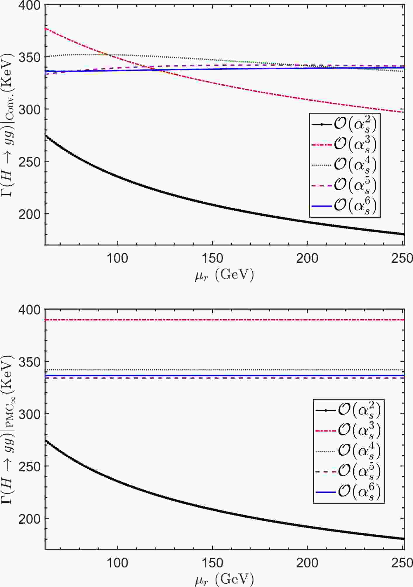
By setting all input parameters to their central values, we first obtained the decay width $ \Gamma (H \to gg) $ up to different $ \alpha_s $-orders under conventional (Conv.) and PMC$ _{\infty} $ scale-setting approaches, as shown in Fig. 1. At the $ \mathcal{O}(\alpha_s^2) $-order level, the perturbative series of $ \Gamma (H \to gg) $ does not have $ \{\beta_i\} $-terms to fix $ \mu_{\rm I} $, and the PMC$ _\infty $ and conventional predictions are the same and scale dependent. Figure 1 shows that the decay width $ \Gamma (H \to gg) $ under conventional scale-setting approach has a strong dependence on $ \mu_r $, which becomes progressively smaller as more loop terms are included. Figure 1 also shows that the decay width $ \Gamma (H \to gg) $ at $ \mathcal{O}(\alpha_s^3) $-order and higher orders under PMC$ _\infty $ scale-setting are independent of any choice of renormalization scale owing to the fact that the scale-dependent noconformal terms have been exactly eliminated.

Figure 1.  (color online) Decay width $ \Gamma (H \to gg) $ under conventional and PMC scale-setting approaches, respectively. The solid line with big dot, dash-dot line, dotted line, dashed line, and solid line are predictions up to $ \mathcal{O}(\alpha_s^2) $, $ \mathcal{O}(\alpha_s^3) $, $ \mathcal{O}(\alpha_s^4) $, $ \mathcal{O}(\alpha_s^5) $, and $ \mathcal{O}(\alpha_s^6) $, respectively.

Next, we present the decay width $ \Gamma (H \to gg) $ up to different loop QCD corrections under conventional and PMC$ _\infty $ scale-setting approaches in Table 1. To show the perturbative property, we define a ratio

	$n=2$	$n=3$	$n=4$	$n=5$	$n=6$	$\kappa_1$	$\kappa_2$	$\kappa_3$	$\kappa_4$
$\Gamma^{\mathcal{O}(\alpha_s^{n})}|_ {\rm{ Conv.}} $	$219.86^{+54.05}_{-39.50}$	$335.46^{+41.34}_{-38.59}$	$349.71^{+2.52}_{-13.68}$	$340.95^{+1.00}_{-7.67}$	$337.45^{+1.94}_{-1.18}$	$[38\%,65\%]$	$[0, 13\%]$	$[0, 4.8\%]$	$[0, 1.0\%]$
$\Gamma^{\mathcal{O}(\alpha_s^{n})}|_{ \rm{ PMC_\infty}} $	$219.86^{+54.05}_{-39.50}$	$389.86$	$342.09$	$334.05$	$336.42$	$[53\%, 95\%]$	$12\%$	$2.4\%$	$0.7\%$

Table 1.  Results for the decay width $\Gamma (H \to gg)$ (unit: keV) and $\kappa_n$ for different loop corrections under conventional and PMC$_\infty$ scale-setting approaches, respectively. The NLO and higher order PMC$_\infty$ predictions are scale independent, while, under the conventional scale-setting approach, the central values are those for $\mu_r=M_H$, and the errors are those for $\mu_r\in[M_H/2, 2M_H].$

which indicates how the "known" prediction $ \Gamma^{\mathcal{O}(\alpha_s^{n+1})} $ is affected by the one-order-higher terms. As for the PMC$ _\infty $ series, we have $ \kappa_1>\kappa_2>\kappa_3>\kappa_4 $ for any choice of $ \mu_r $, indicating that the relative difference between the two nearby orders becomes smaller when more loop terms are included. This feature is consistent with the perturbative nature of the series and indicates that one can obtain more precise predictions by including more loop terms. Concerning the conventional series, as shown in Fig. 2, there are crossovers for $ \kappa_{2,3,4} $ within the range of $ \mu_r\in[M_H/2, 2M_H] $, and the ratios vary from $ 0 $ to $ 13\% $, $ 4.8\% $, and $ 1.0\% $ for $ \kappa_2 $, $ \kappa_3 $, and $ \kappa_4 $, respectively.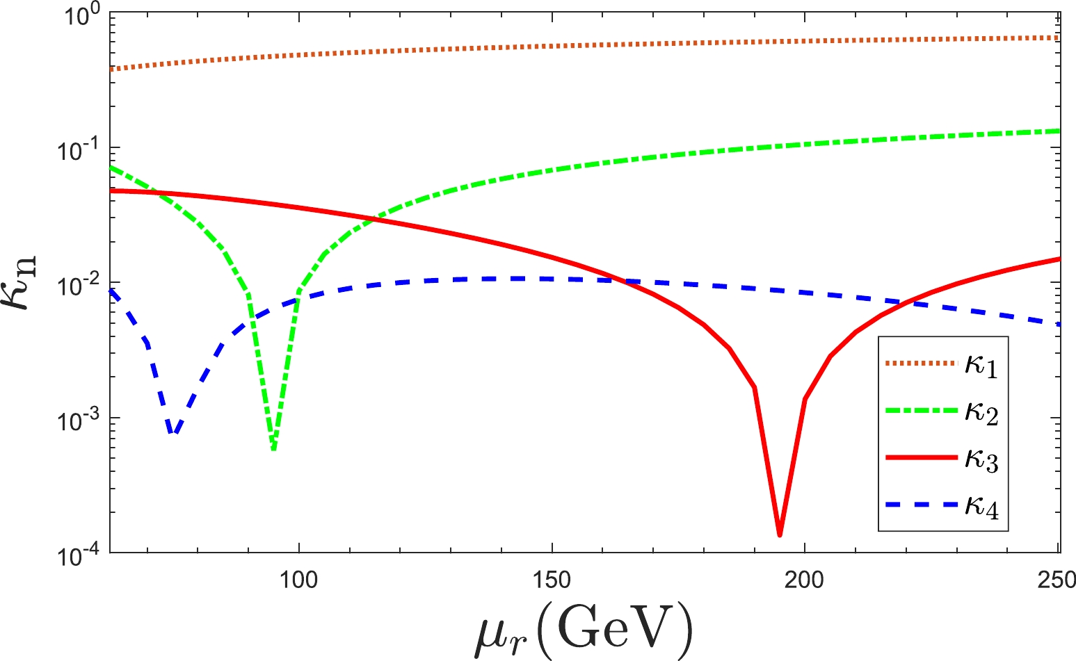

Figure 2.  (color online) Results for the ratio $ \kappa_n $ versus renormalization scale $ \mu_r $ under conventional scale-setting approach for different loop corrections. The ratios under PMC $ _\infty $ approach are scale invariant.

Moreover, to show the convergence of the perturbative series explicitly, we present the magnitude of each loop term for the four-loop approximants $ \Gamma^{\mathcal{O}(\alpha_s^{6})} $ in Table 2, which shows that the relative importance of the LO-terms: NLO-terms: N$ ^2 $LO-terms: N$ ^3 $LO-terms: N$ ^4 $LO-terms for the conventional series is

	$\rm LO$	$\rm NLO$	$\rm N^2LO$	$\rm N^3LO$	$\rm N^4LO$	$\rm Total$
$\Gamma^{\mathcal{O}(\alpha_s^{6})}|_{ \rm{ Conv.}} $	$218.66^{-40.95}_{+57.39}$	$116.62^{+2.08}_{-15.59}$	$14.44^{+25.23}_{-41.60}$	$-8.70^{+13.84}_{-8.02}$	$-3.57^{+1.74}_{+6.64}$	$337.45^{+1.94}_{-1.18}$
$\Gamma^{\mathcal{O}(\alpha_s^{6})}|_ {\rm {PMC_\infty}} $	299.57	95.22	$-$41.82	$-$19.59	3.04	336.42
$\Gamma^{\mathcal{O}(\alpha_s^{6})}|_ {\rm{ PMCm}} $	289.83$^{+0.96}_{-0.24}$	91.19$^{-0.51}_{+0.29}$	$-$31.78$^{+0.30}_{-0.11}$	$-$13.36	1.92	337.80$^{+0.75}_{-0.06}$

Table 2.  Values (unit: keV) of each loop-term (LO, NLO, N $^2$LO, and N $^3$LO) for the four-loop prediction $\Gamma^{\mathcal{O}(\alpha_s^{6})}$ under the conventional, PMC$_\infty$ scale-setting, and PMCm scale-setting approaches, respectively. The PMC$_\infty$ predictions are scale independent, while, under the conventional and PMCm scale-setting approaches, the central values are those for $\mu_r=M_H$, and the errors are those for $\mu_r\in[M_H/2, 2M_H].$

where the central values are those for $ \mu_r=M_H $, and the errors are those for $ \mu_r\in [\frac{1}{2}M_H, 2M_H] $. The scale dependence for each loop term is large. However, owing to the cancellation of scale dependence among different orders, the net scale dependence is small, e.g., $ (^{+0.6\%}_{-0.3\%}) $ for $ \mu_r\in [\frac{1}{2}M_H, 2M_H] $. In contrast, there is no renormalization scale dependence for each loop term of the PMC$ _{\infty} $ prediction $ \Gamma^{\mathcal{O}(\alpha_s^{6})} $. More explicitly, we also present the value of each loop-term (LO, NLO, N $ ^2 $LO, N$ ^3 $LO, or N $ ^4 $LO) for $ \Gamma^{\mathcal{O}(\alpha_s^{6})} $ under the PMC$ _{\infty} $ approach in Table 2. At the four-loop level, the PMC$ _\infty $ series already represents good convergent behavior, and the relative importance of the LO-terms: NLO-terms: N$ ^2 $LO-terms: N$ ^3 $LO-terms: N$ ^4 $LO-terms becomes

whose magnitudes are scale invariant, indicating that the PMC$ _\infty $ perturbative series represents the intrinsic perturbative behavior of $ \Gamma (H \to gg) $. For comparison, we also show the numerical results under the PMC multi-scale approach (PMCm) in Table 2, which still has some residual scale-dependence. However, its numerical effect is smaller than that of the conventional approach. Detailed formulas for the PMCm approach can be found in Ref. [22].

Now, after eliminating the renormalization scale ambiguities, there are still some other error sources for the pQCD prediction of the total decay width, such as the $ \alpha_s $ fixed-point error $ \Delta\alpha_s(M_Z) $, the Higgs mass uncertainty $ \Delta M_{H} $, and the top-quark pole mass uncertainty $ \Delta M_t $. Up to $ \alpha_s^6 $-order, we have

where the errors are $ \Delta \alpha_s(M_Z) =\pm 0.0009 $ (which leads to $ \Lambda^{n_f=5}_{\rm mMOM}=362.0^{+36.6}_{-18.0} $ MeV), $ \Delta M_{H}=\pm0.17 $ GeV, and $ \Delta M_t=\pm0.7 $ GeV, respectively. Here, the conventional predictions are achieved by fixing $ \mu_r=M_H $.

Using the PMC$ _\infty $ approach, the PMC scales at each order are no longer evaluated as a perturbative series, thus avoiding the first type of residual scale dependence. As mentioned above, all the PMC$ _\infty $ scales are around $ M_H \exp(-5/6)\sim 54 $ GeV, so the second type of residual scale dependence is small owing to the convergent behavior at higher orders. As a further step of making a conservative estimation on the contributions from the uncalculated $ {n+1}_{\rm th} $-order terms, we set its PMC$ _\infty $ scale $ \mu_{n} $ to be within the region of the latest determined PMC$ _\infty $ scale $ \mu_{n-1} $, e.g., $ \mu_{n}\in[\mu_{n-1}/2, 2\mu_{n-1}] $, and set $\Delta\Gamma^{{\mathcal O}(\alpha_s^{i+1})}|_{\rm PMC_\infty}= \pm\frac{M_H^3 G_F}{36\sqrt{ 2}\pi}|C_{i, {\rm Conf}}a^{i+2}_s(\mu_{i+1})|_{\rm MAX}$ with $ i=I,II, III,IV, V $, respectively. Numerically, we obtained $\Delta\Gamma^{{\mathcal O}(\alpha_s^{2})}|_{\rm PMC_\infty}= \pm 2.99$ keV, $ \Delta\Gamma^{{\mathcal O}(\alpha_s^{3})}|_{\rm PMC_\infty}=\pm 1.80 $ keV, $\Delta\Gamma^{{\mathcal O}(\alpha_s^{4})}|_{\rm PMC_\infty}= \pm 1.25$ keV, $ \Delta\Gamma^{{\mathcal O}(\alpha_s^{5})}|_{\rm PMC_\infty}=\pm 0.47 $ keV, and $ \Delta\Gamma^{{\mathcal O}(\alpha_s^{6})}|_{\rm PMC_\infty}=\pm 0.09 $ keV. Note that the estimated errors may underestimate the contributions listed in Table 1, which need to be multiplied by $ \{57, 27, 6, 5\} $, respectively. Thus, the numerical results for $ \Delta\Gamma^{{\mathcal O}(\alpha_s^{6})}|_{\rm PMC_\infty} $ need to be multiplied by $ 5 $ as analogy. Similarly, one can obtain the corresponding values for the conventional scale-setting approach, which are $ \pm 11.98 $ keV, $ \pm 4.60 $ keV, $ \pm 1.40 $ keV, $ \pm 0.73 $ keV, and $ \pm 0.14 $ keV, respectively. To match the center values shown in Table 1, these values need to be multiplied by $ \{10, 3, 6, 5\} $. Moreover, the numerical results for $ \Delta\Gamma^{{\mathcal O}(\alpha_s^{6})}|_{\rm Conv.} $ need to be multiplied by $ 5 $ as analogy. Those values are slightly larger than those of PMC$ _\infty $ owing to a larger perturbative coefficient $ C_k $ than the conform coefficient at each order, even if it is compensated by a smaller $ \alpha_s $ value.

As a summary, we have presented a detailed analysis of the Higgs-boson decay $ H \to gg $ up to $ \alpha_s^6 $-order, and we obtain

where the errors are squared averages of those from $ \Delta \alpha_s(M_Z) $, $ \Delta M_{H} $, $ \Delta M_t $, and the uncertainty of the renormalization scale within the region of $ \left[{M_H}/{2},2 M_H\right] $. The errors are dominated by $ \Delta \alpha_s(M_Z) $, followed by the choice of renormalization scale and accuracy of Higgs mass. If the value of $ \alpha_s(M_Z) $ can be measured accurately to avoid the error from $ \Delta \alpha_s(M_Z) $, we will obtain

The Higgs-boson decay $ H \to gg $ provides another successful example for the application of the PMC$ _\infty $ scale-setting method to high-energy processes. Up to N$ ^4 $LO QCD corrections, the pQCD predictions under PMC$ _\infty $ and conventional scale-setting approaches are consistent with each other. However, the conventional renormalization scale uncertainties are still sizable, i.e., approximately $ 1\% $ when varying the renormalization scale $ \mu_r $ within the range of $ [\frac{1}{2}M_H, 2M_H] $. By applying PMC$ _\infty $, the $ \alpha_s $ values at lower orders are definitely fixed by the requirement of intrinsic conformality, the conventional renormalization scale ambiguity is eliminated, and the residual scale dependence from the original PMC multi-scale-setting approach is also highly suppressed. Thus, a more precise test of the SM can be achieved.