


 Abstract
 HTML
HTML Reference
 Related
 PDF
PDF


-
Effective field theory (EFT) has wide applications in various aspects of physics. It serves as a powerful tool to understand the emergent coarse-graining behavior, where the underlying system has sophisticated patterns or is strongly coupled, such as superconductivity [1], fractional quantum hall effect [2], and low energy QCD [3]. Meanwhile, EFT provides a model-independent method to categorize and parametrize possible unknown physics from the ultraviolet (UV) band. In this case, our best example is the Standard Model (SM) EFT, which becomes a basic paradigm of exploring the imprints of beyond the SM effects.
One essential step in an EFT calculation is the identification of a complete operator basis [4–8]. To construct the full set of independent operators in quantum field theory, one has to eliminate the redundancies from the equation of motion (EOM) and integration by parts (IBP), which yield relations between operators. Previously, researchers relied on symmetry [9–14] in the SM to eliminate those redundancies and encode enumeration of operators in a Hilbert series. Nevertheless, those methods do not give exact expressions of all operators and are not naturally directed to the SMEFT calculations.
In this paper, we introduce a novel way to present all independent operators, which is based on the on-shell amplitude method [15]. Instead of using symmetries to deal with the EOM and IBP, we can write down all complete local on-shell amplitudes respecting Lorentz symmetry, SM gauge symmetry, and the spin-statistics theorem. Those on-shell amplitudes are in one to one correspondence with the operators, which naturally form a new amplitude basis. Our key observation is that, for amplitude basis, the elimination of EOM and IBP redundancies are trivially realized by external leg on-shell conditions and momentum conservation, as naturally inherited from the on-shell amplitudes. This approach was used recently to infer the EFT Lagrangian for theories with a spin-0 or 1 singlet coupled to gluons [16].
Our method has several advantages. When using the on-shell amplitude method, the root of our amplitude basis comprises the unfactorizable on-shell amplitudes from locality (positive power of Madelstam variables without poles). We start directly with the computation of unfactorizable amplitudes from spin helicity formulism, thus automatically providing the basic building blocks of the EFT calculation, and advanced techniques, such as recursion relations or unitarity cuts, can be used naturally. Indeed, our method also greatly simplifies the calculation. The amplitude basis at d=6 for SMEFT corresponds to the Warsaw basis, except for some linear combinations; the derivation for this is presented in a later section of the paper.
The rest of the paper is organized as follows. We first discuss the general structure of the amplitude basis and outline the rules of constructing the complete set of amplitude basis in a given dimension. Using these tools, we explicitly construct the amplitude bases for SMEFT at
$ d=5 $ and$ 6 $ and map them to the corresponding operators. Finally, we present our conclusions. -
We start from the S-matrix program, which uses a set of low point amplitudes as building blocks, and construct higher point amplitudes by matching their residues using recursion relations. Because of the renormalizability, the finite set of low point amplitudes is sufficient as the theory input. However, in an non-renormalizable theory such as SMEFT, the irrelevant operators
$ \mathcal{O} $ are independent interactions, which cannot be constructed on-shell by recursion relations without the help of symmetries. Therefore, those independent amplitudes should be viewed as the input basis of the theory, which correspond to the independent set of operators and can be classified by their dimensions.We build a one-to-one correspondence between the amplitude basis and irrelevant operators
$ \mathcal{O} $ by enforcing that all fields from$ \mathcal{O} $ are on shell. The gauge symmetry, which reflects the redundancy, can be used to reduce the independent amplitudes. Only the leading contact on-shell amplitudes that have the minimal fields from$ \mathcal{O} $ are sufficient to fully construct all on-shell amplitudes for a given dimension [17]. Indeed, this is the same as the famous example of Yang-Mills theory; the cubic term$ A^2 \partial A $ captures the full information for the on-shell amplitudes, and the 4-point on-shell amplitudes are not independent from recursion relations (the existence of 4-point contact interactions from$ A^4 $ simply has no on-shell information). Since the above arguments only exploit gauge invariance, they should apply to the non-renormalizable theory.From Lorentz symmetry, the basic building blocks to construct the effective operators are
$F^\pm_{\mu \nu} \equiv \dfrac{1}{2}(F_{\mu \nu} \pm {\rm i} \tilde{F}_{\mu \nu} )$ ($ \tilde{F}_{\mu \nu} \equiv \epsilon_{\mu \nu \rho \sigma} F^{\rho \sigma} $ ),$ \psi_L $ ,$ \psi^c_L $ , ϕ, and covariant derivative$ D_\mu $ which transforms under Lorentz group$S U(2)_L \times S U(2)_R \equiv S O(3,1)$ as$ (1,0) $ ,$ (0,1) $ ,$ (1/2,0) $ ,$ (0,1/2) $ , and$ (0,0) $ . As we have mentioned above, in the amplitude operator correspondence, only the leading contact on-shell amplitudes are taken into account; this suggests that we take "$ F_{\mu \nu} \rightarrow \partial_\mu A_\nu - \partial_\nu A_\mu $ " and "$ D_\mu \rightarrow \partial_\mu $ " to construct those effective operators.There are two redundancies in the effective operators from the Equation of Motion (EOM) and Integration by Part (IBP). However, in our amplitude basis, these are resolved automatically because of the on shell condition and momentum conservation. The EOM for each field will transmit the operators involving the derivatives of such a field into other operators. In our definition, the on shell condition
$ p^2=0 $ suggests that operators involving$ □\phi $ ,$\not D/\psi$ , or$ D_{\mu}F^{\mu\nu} $ should vanish in the amplitude basis; thus, there is no such redundancy. For IBP in the amplitude basis, two operators differing by a total derivative are equivalent as the total derivative is the sum of all external momenta, which equals zero.The general on-shell scattering amplitude should have the following form:
$ \begin{array}{*{20}{l}} { \mathcal{M}_{\{\alpha\}} = f(\lambda_i,\tilde\lambda_i) g(s_{ij}) T_{\{\alpha\}}, } \end{array} $

(1) where
$ \lambda_i,\tilde\lambda_i $ are helicity spinors of the ith leg and Mandelstam variable$ s_{ij} \equiv 2p_i.p_j $ (see more details about spinor formalism in App. A.1), f is the little group weight function, which is a function of spinor products$ [ij]=\lambda_i\epsilon\lambda_j $ and$ \langle {ij} \rangle=\tilde\lambda_i\epsilon\tilde\lambda_j $ , g is the little group invariant function, and T is the group factor, bearing all the internal group indices of the external legs$ \{\alpha\} $ and forming invariant tensors. For the amplitude basis in a non-renormalizable theory, all spinor products in f and g have positive powers, which have no physical poles in Mandelstam variables and cannot be factorized into smaller building blocks due to locality [18].According to dimension counting, it is easy to obtain the operator dimension d of an amplitude basis
$ \begin{array}{*{20}{l}} { d = n+m =n + [f]+[g], } \end{array} $

(2) where n is the number of legs, and
$ [f] $ and$ [g] $ are the dimensions of f and g, where$ [g] $ is always an even integer. The scattering processes are classified in terms of fermion number$ n_\psi $ and gauge boson number$ n_A $ . Each fermion contributes one helicity spinor, and each gauge boson contributes two; thus, the number of spinor products is at least$ m \geq \dfrac{1}{2}n_\psi+n_A $ . Using Eq. (2), we have$ { \frac{3}{2}n_\psi + 2 n_A \leq d }, $

(3) which gives finite possibilities below a certain dimension. For instance, to obtain an amplitude basis below
$ d=6 $ , we need scattering amplitudes with$ (n_\psi,n_A) $ satisfying$ \dfrac{3}{2}n_\psi + 2n_A \leq 6 $ . We list all possible amplitude bases in$ (n_\psi,n_A, h) $ , where h is the total helicity with$ h \ge 0 $ , in Table 1; we can just flip the helicity for$ h<0 $ . We leave the scalar number unspecified to shorten the list because adding a scalar does not change the form of the Lorentz factor. For each$ (n_\psi, n_A, h) $ , we examine all possible helicity combinations (up to the conjugation).$ (n_\psi,n_A,h) $ 

Primary amplitude $m_{\min}$ 

$ n_s $ 

$d_{\min}$ 

(0,0,0) $ f(\phi^{n_s})=1 $ 

0 $ n_s \geqslant 3 $ 

3 (0,2,2) $ f(A^+A^+\phi^{n_s}) = [12]^2 $ 

2 5 (0,3,3) $ f(A^+A^+A^+) = [12][23][31] $ 

3 6 (2,0,1) $ f(\psi^+\psi^+\phi^{n_s}) = [12] $ 

1 4 (2,0,0) $ f(\psi^+\psi^-\phi^{2}) = [1|p_3| {2} \rangle $ 

2 $ n_s \geqslant 2 $ 

6 (2,1,2) $ f(A^+\psi^+\psi^+ \phi^{n_s}) = [12][13] $ 

2 5 (4,0,2) $ f(\psi^+\psi^+\psi^+\psi^+) = [12][34]^* $ 

2 6 (4,0,0) $ f(\psi^+\psi^+\psi^-\psi^-) = [12]\langle {34} \rangle $ 

2 6 Table 1. All classes of the amplitude basis with
$ d \le 6 $ . The$ * $ for the$ (4,0,2) $ case stands for multiple ways of spinor contraction.For a given helicity assignment, we can write down the net powers of helicity spinors of all legs. For instance
$ \begin{aligned}[b]& f(\psi^+\psi^+\phi^2) \sim \lambda_1\lambda_2, \\ & f(\psi^+\psi^-\phi^2) \sim \lambda_1\tilde\lambda_2. \end{aligned} $

(4) To contract the spinor indices, we use the complete set of Clifford algebra
$\{1,\sigma^{\mu},\sigma^{\mu\nu},\sigma^{\mu\nu\rho},{\rm i}\epsilon^{\mu\nu\rho\xi} \}$ to construct bilinears. Specifically,$ \{1,\sigma^{\mu\nu}\} $ can be used to contract two λs or two$ \tilde{\lambda} $ s, while$ \{\sigma^{\mu},\sigma^{\mu\nu\rho}\} $ can be used to contract a λ and a$ \tilde\lambda $ . The more spacetime indices ($ \mu,\nu,\dots $ ) a bilinear has, the more momenta we need to add to contract with them, which increases m. For instance, to contract a$ \lambda_i $ and a$ \tilde\lambda_j $ , the lowest dimension combination we can use is$ (\lambda_i\sigma^{\mu}\tilde{\lambda}_j) p_{k\mu} \equiv [i|p_k| {j} \rangle = [ik]\langle {kj} \rangle $ . Following this rule, the lowest dimension amplitudes for the cases (4) are$ \begin{aligned}[b]& f(\psi^+\psi^+\phi^2) \sim (\lambda_1 \epsilon \lambda_2) \equiv [12], \\& f(\psi^+\psi^-\phi^2) \sim (\lambda_1 \epsilon \sigma^{\mu}\tilde\lambda_2)p_{3 \mu} \equiv [1|p_3 | {2} \rangle. \end{aligned} $

(5) Moreover, Mandelstam variables can be added freely to g, as it is helicity blind. For each helicity assignment, there is a kinematic factor with minimum m and thus a minimum dimension d, which we call primary amplitude. It is the leading amplitude for a given set of scattering states.
We work out all primary amplitudes in Table 1 for
$ d \le 6 $ . For the$ (4,0,2) $ case, there are different types of spinor contraction combinations, and we can define$ f^{\pm}(\psi^+\psi^+\psi^+\psi^+) = ([13][24] \pm [14][23]) $ after applying the Schouten identity$ [12][34] + [13][42] + [14][23] = 0 $ . -
The results in the previous section are simple consequences of Lorentz invariance, gauge invariance, and locality. When applying to SM matter fields in Table 2, one has to take into account the SM gauge quantum numbers and respect Fermi or Boson statistics for identical fields. In this section, we explicitly construct the complete amplitude basis at dim-5 and dim-
$ 6 $ for SM EFT.$ SU(3)_c $ 

$ SU(2)_L $ 

$ U(1)_Y $ 

$ G_A^\pm $ 

$ \mathbf{3} $ 

$ \mathbf{1} $ 

0 $ W_i^\pm $ 

$ \mathbf{1} $ 

$ \mathbf{3} $ 

0 $ B^\pm $ 

$ \mathbf{1} $ 

$ \mathbf{1} $ 

0 $ Q_{a\alpha} $ 

$ \mathbf{3} $ 

$ \mathbf{2} $ 

1/6 $ u_{\dot{a}} $ 

$ \mathbf{\bar{3}} $ 

$ \mathbf{1} $ 

−2/3 $ d_{\dot{a}} $ 

$ \mathbf{\bar{3}} $ 

$ \mathbf{1} $ 

1/3 $ L_{\alpha} $ 

$ \mathbf{1} $ 

$ \mathbf{2} $ 

−1/2 e $ \mathbf{1} $ 

$ \mathbf{1} $ 

1 $ H_{\alpha} $ 

$ \mathbf{1} $ 

$ \mathbf{2} $ 

1/2 Table 2. Standard Model particle content is listed according to their representations under gauge group
$S U(3)_c \times $ $ S U(2)_L \times U(1)_Y$ . All fermions are in the form of left hand.To count the dim-5 amplitude basis in SM EFT, we need to combine the amplitudes in Table 1 and appropriate group factors. Group factors are not always unique for a given set of group indices, and when there are multiple choices, we use superscripts to label them. In particular, superscripts
$ \pm $ indicate the permutation symmetry among the same type of indices, such as$ T^{\pm}_{\alpha\beta\dot\alpha\dot\beta} = \dfrac{1}{2}(\delta_{\alpha\dot\alpha}\delta_{\beta\dot\beta} \pm \delta_{\alpha\dot\beta}\delta_{\beta\dot\alpha}) $ . Among the kinematic factors in Table 1, we find that only the$ f(\psi^+\psi^+\phi^2) $ combination is the SM gauge singelt, which is$ \begin{array}{*{20}{l}} { \mathcal{M}(L_{\alpha}L_{\beta}H_{\gamma}H_{\delta}) = [12] (\epsilon_{\alpha\gamma}\epsilon_{\beta\delta} + \epsilon_{\alpha\delta}\epsilon_{\beta\gamma}) , } \end{array} $

(6) where the group factor is chosen to satisfy the spin statistics. Together with its conjugate
$ f(\psi^-\psi^-\phi^2) $ with opposite helicity, we find the only 2 dim-5 amplitude bases in SM EFT, which are the Weinberg operators$\mathcal{O}^{(5)} = \dfrac{1}{\Lambda}(H L)^2 + \rm h.c. \,$ .The dim-6 amplitude bases in SM EFT are obtained in the same way. It is interesting that the classes of our amplitude basis in Table 1 already reproduce the classes of operators summarized in Ref. [5] as the Warsaw basis. Because we choose the group factor basis and Mandelstam variables according to the permutation symmetry, the resultant amplitude basis for the same scattering states we get might be the linear combination of the operators defined in the Warsaw basis. We list the correspondence as follows:
1. Class
$ \mathcal{M}(\phi^{n_s}) $ ($ \mathcal{O}\sim\varphi^6 $ and$ \varphi^4D^2 $ ):Operator Amplitude Basis $ \mathcal{O}_H $ 

$ \mathcal{M}(H^3_{\alpha\beta\gamma}H^{\dagger3}_{\dot\alpha\dot\beta\dot\gamma}) = T^+_{\alpha\beta\gamma\dot\alpha\dot\beta\dot\gamma} $ 

$2\mathcal{O}_{HD}-\mathcal{O}_{H\square}$ 

$ \mathcal{M}^+(H^2_{\alpha\beta}H^{\dagger2}_{\dot\alpha\dot\beta}) = s_{12}T^+_{\alpha\beta\dot\alpha\dot\beta} $ 

$2\mathcal{O}_{HD}+\mathcal{O}_{H\square}$ 

$ \mathcal{M}^-(H^2_{\alpha\beta}H^{\dagger2}_{\dot\alpha\dot\beta}) = (s_{13} - s_{23})T^-_{\alpha\beta\dot\alpha\dot\beta} $ 

Where
$T^+_{\alpha\beta\gamma\dot\alpha\dot\beta\dot\gamma} \equiv \delta_{\alpha \dot\alpha} \delta_{\beta \dot\beta} \delta_{\gamma \dot \gamma} +\delta_{\beta \dot\alpha} \delta_{\alpha \dot\beta} \delta_{\gamma \dot \gamma} + \delta_{\gamma \dot\alpha} \delta_{\beta \dot\beta} \delta_{\alpha \dot \gamma} + \delta_{\beta \dot\alpha} \delta_{\gamma \dot\beta} \delta_{\alpha \dot \gamma} + \delta_{\alpha \dot\alpha} \delta_{\gamma \dot\beta} \delta_{\beta \dot \gamma} +\delta_{\gamma \dot\alpha} \delta_{\alpha \dot\beta} \delta_{\beta \dot \gamma}$ is fully symmetric for$S U(2)_L$ indices$ \alpha\beta\gamma $ and$ \dot\alpha\dot\beta\dot\gamma $ .$ T^\pm _{\alpha\beta\dot\alpha\dot\beta} \equiv \delta_{\alpha \dot\alpha} \delta_{\beta \dot\beta} \pm \delta_{\beta \dot\alpha} \delta_{\alpha \dot\beta} $ is the (ant-)symmetric group structure for indices$ \alpha\beta $ and$ \dot \alpha \dot \beta $ .$ s_{12} $ and$ s_{12} - s_{23} $ are the symmetric and antisymmetric Mandelstam variables at the order s.2. Class
$ \mathcal{M}(A^+A^+\phi^2) $ and$ \mathcal{M}(A^-A^-\phi^2) $ ($ \mathcal{O}\sim X^2\varphi^2 $ ):Instead of operators with definite CP, the amplitude bases are more naturally expressed for definite chirality. They have easy linear relations.
Warsaw Amplitude Basis $ \mathcal{O}_{HB}+ \mathcal{O}_{H\tilde{B}} $ 

$ \mathcal{M}(B^{+}B^{+}H_{\alpha}H^{\dagger}_{\dot\alpha}) = [12]^2\delta_{\alpha\dot\alpha} $ 

$ \mathcal{O}_{HB}- \mathcal{O}_{H\tilde{B}} $ 

$ \mathcal{M}(B^{-}B^{-}H_{\alpha}H^{\dagger}_{\dot\alpha}) = \langle12\rangle^2\delta_{\alpha\dot\alpha} $ 

$ \mathcal{O}_{HWB}+\mathcal{O}_{H\tilde{W}B} $ 

$ \mathcal{M}(B^{+}W^{i+}H_{\alpha}H^{\dagger}_{\dot\beta}) = [12]^2\tau^i_{\alpha\dot\beta} $ 

$ \mathcal{O}_{HWB}- \mathcal{O}_{H\tilde{W}B} $ 

$ \mathcal{M}(B^{-}W^{i-}H_{\alpha}H^{\dagger}_{\dot\beta}) = \langle12\rangle^2\tau^i_{\alpha\dot\beta} $ 

$ \mathcal{O}_{HW} + \mathcal{O}_{H\tilde{W}} $ 

$ \mathcal{M}(W^{i+}W^{j+}H_{\alpha}H^{\dagger}_{\dot\beta}) = [12]^2 T^{ij+}_{\alpha\dot\beta} $ 

$ \mathcal{O}_{HW}- \mathcal{O}_{H\tilde{W}} $ 

$ \mathcal{M}(W^{i-}W^{j-}H_{\alpha}H^{\dagger}_{\dot\beta}) =\langle12\rangle^2T^{ij+}_{\alpha\dot\beta} $ 

$ \mathcal{O}_{HG}+ \mathcal{O}_{H\tilde{G}} $ 

$ \mathcal{M}(G^{A+}G^{B+}H_{\alpha}H^{\dagger}_{\dot\beta}) = [12]^2 T^{AB+}_{\alpha\dot\beta} $ 

$ \mathcal{O}_{HG}- \mathcal{O}_{H\tilde{G}} $ 

$ \mathcal{M}(G^{A-}G^{B-}H_{\alpha}H^{\dagger}_{\dot\beta}) = \langle12\rangle^2T^{AB+}_{\alpha\dot\beta} $ 

Where
$ \tau^i $ is the Pauli matrix,$ T^{ij+}_{\alpha\dot\beta} \equiv \delta^{ij} \delta_{\alpha\dot\beta} $ , and$T^{AB+}_{\alpha\dot\beta} \equiv \delta^{AB} \delta_{\alpha\dot\beta}$ .3. Class
$ \mathcal{M}(A^+A^+A^+) $ and$ \mathcal{M}(A^-A^-A^-) $ ($ \mathcal{O}\sim X^3 $ ):Warsaw Amplitude Basis $ \mathcal{O}_W + \mathcal{O}_{\tilde{W}} $ 

$ \mathcal{M}(W^{i+}W^{j+}W^{k+}) = [12][23][31]\epsilon^{ijk} $ 

$ \mathcal{O}_W - \mathcal{O}_{\tilde{W}} $ 

$ \mathcal{M}(W^{i-}W^{j-}W^{k-}) = \langle12\rangle \langle23\rangle \langle31\rangle\epsilon^{ijk} $ 

$ \mathcal{O}_G + \mathcal{O}_{\tilde{G}} $ 

$ \mathcal{M}(G^{A+}G^{B+}G^{C+}) = [12][23][31] f^{ABC} $ 

$ \mathcal{O}_G - \mathcal{O}_{\tilde{G}} $ 

$ \mathcal{M}(G^{A-}G^{B-}G^{C-}) =\langle12\rangle \langle23\rangle \langle31\rangle f^{ABC} $ 

Where
$ \epsilon^{ijk} $ and$ f^{ABC} $ are the$ S U(2)_L $ and$ S U(3)_c $ structure constants.4. Class
$ \mathcal{M}(\psi^+\psi^+\phi^3) $ ($ \mathcal{O}\sim \psi^2\varphi^3 $ ) + h.c.:Warsaw Amplitude Basis $ \mathcal{O}_{eH} $ 

$ \mathcal{M}(L_{\alpha}eH_{\beta}H^{\dagger2}_{\dot{\alpha}\dot{\beta}}) = [12]T^+_{\alpha\beta\dot\alpha\dot\beta} $ 

$ \mathcal{O}_{dH} $ 

$ \mathcal{M}(Q_{a\alpha}d_{\dot{a}}H_{\beta}H^{\dagger2}_{\dot{\alpha}\dot{\beta}}) = [12]T^+_{\alpha\beta\dot\alpha\dot\beta}\delta_{a\dot{a}} $ 

$ \mathcal{O}_{uH} $ 

$ \mathcal{M}(Q_{a\alpha}u_{\dot{a}}H^2_{\beta\gamma}H^{\dagger}_{\dot{\alpha}}) = [12]T^+_{\alpha(\beta\gamma)\dot\alpha}\delta_{a\dot{a}} $ 

Where the group structure
$ T^+_{\alpha(\beta\gamma)\dot\alpha}\equiv \epsilon_{\alpha \beta} \delta_{\gamma \dot\alpha} +\epsilon_{\alpha \gamma} \delta_{\beta \dot\alpha} $ is symmetric for indices β and γ. If we flip the helicity of fermions, we get another three independent amplitude bases in the class of$ \mathcal{M}(\psi^- \psi^- \phi^3) $ , which is the conjugation of above operator basis. The expressions of these new amplitude bases are obtained by replacing the helicity factor$ [12] $ with$ \langle 12 \rangle $ in above expressions.5. Class
$ \mathcal{M}(\psi^+\psi^-\phi^2) $ ($ \mathcal{O}\sim \psi^2\varphi^2D $ ):Note that momentum conservation implies that
$ [1|p_3| {2} \rangle = \frac{1}{2}[1|p_3-p_4| {2} \rangle $ for$ n=4 $ and is antisymmetric for the two scalars ($ [1|p_3 +p_4| | {2} \rangle=0 $ ). Hence, there is only one independent term.Warsaw Amplitude Basis $ \mathcal{O}_{He} $ 

$ \mathcal{M}(ee^{\dagger}H_{\alpha}H^{\dagger}_{\dot\alpha}) = [1|p_3| {2} \rangle \delta_{\alpha\dot\alpha} $ 

$ \mathcal{O}_{Hu} $ 

$ \mathcal{M}(u_{\dot{a}}u^{\dagger}_{a}H_{\alpha}H^{\dagger}_{\dot\alpha}) = [1|p_3| {2} \rangle \delta_{\alpha\dot\alpha}\delta_{a\dot{a}} $ 

$ \mathcal{O}_{Hd} $ 

$ \mathcal{M}(d_{\dot{a}}d^{\dagger}_{a}H_{\alpha}H^{\dagger}_{\dot\alpha}) = [1|p_3| {2} \rangle \delta_{\alpha\dot\alpha}\delta_{a\dot{a}} $ 

$ \mathcal{O}_{Hud} $ 

$ \mathcal{M}(d_{\dot{a}}u^{\dagger}_{a}H^2_{\alpha\beta}) = \dfrac{1}{2}[1|p_3-p_4| {2} \rangle\epsilon_{\alpha\beta}\delta_{a\dot{a}} $ 

$ \mathcal{O}_{Hud}^\dagger $ 

$ \mathcal{M}( u_{\dot{a}}d^{\dagger}_{a}H^{\dagger 2}_{\dot \alpha \dot \beta}) = \dfrac{1}{2}[1|p_3-p_4| {2} \rangle\epsilon_{\dot\alpha \dot \beta}\delta_{a\dot{a}} $ 

$ \mathcal{O}_{HL}^{(3)} + \dfrac{3}{4}\mathcal{O}_{HL}^{(1)} $ 

$ \mathcal{M}^+(L_{\alpha}L^{\dagger}_{\dot\alpha}H_{\beta}H^{\dagger}_{\dot\beta}) = [1|p_3| {2} \rangle T^+_{\alpha\beta\dot\alpha\dot\beta} $ 

$ \mathcal{O}_{HL}^{(3)} - \dfrac{1}{4}\mathcal{O}_{HL}^{(1)} $ 

$ \mathcal{M}^-(L_{\alpha}L^{\dagger}_{\dot\alpha}H_{\beta}H^{\dagger}_{\dot\beta}) = [1|p_3| {2} \rangle T^-_{\alpha\beta\dot\alpha\dot\beta} $ 

$ \mathcal{O}_{HQ}^{(3)} + \dfrac{3}{4}\mathcal{O}_{HQ}^{(1)} $ 

$ \mathcal{M}^+(Q_{a\alpha}Q^{\dagger}_{\dot{a}\dot\alpha}H_{\beta}H^{\dagger}_{\dot\beta}) = [1|p_3| {2} \rangle T^+_{\alpha\beta\dot\alpha\dot\beta}\delta_{a\dot{a}} $ 

$ \mathcal{O}_{HQ}^{(3)} - \dfrac{1}{4}\mathcal{O}_{HQ}^{(1)} $ 

$ \mathcal{M}^-(Q_{a\alpha}Q^{\dagger}_{\dot{a}\dot\alpha}H_{\beta}H^{\dagger}_{\dot\beta}) = [1|p_3| {2} \rangle T^-_{\alpha\beta\dot\alpha\dot\beta}\delta_{a\dot{a}} $ 

6. Class
$ \mathcal{M}(A^+\psi^+\psi^+\phi) $ ($ \mathcal{O}\sim \psi^2X\varphi $ ) +h.c.:Warsaw Amplitude Basis $ \mathcal{O}_{eB} $ 

$ \mathcal{M}(B^+eL_{\alpha}H^{\dagger}_{\dot\alpha}) = [12][13]\delta_{\alpha\dot\alpha} $ 

$ \mathcal{O}_{dB} $ 

$ \mathcal{M}(B^+d_{\dot{a}}Q_{a\alpha}H^{\dagger}_{\dot\alpha}) = [12][13] \delta_{\alpha\dot\alpha}\delta_{a\dot{a}} $ 

$ \mathcal{O}_{dG} $ 

$ \mathcal{M}(G^{A+}d_{\dot{b}}Q_{a\alpha}H^{\dagger}_{\dot\alpha}) = [12][13]\delta_{\alpha\dot\alpha}\lambda^A_{a\dot{b}} $ 

$ \mathcal{O}_{eW} $ 

$ \mathcal{M}(W^{i+}eL_{\alpha}H^{\dagger}_{\dot\beta}) = [12][13]\tau^i_{\alpha\dot\beta} $ 

$ \mathcal{O}_{dW} $ 

$ \mathcal{M}(W^{i+}d_{\dot{a}}Q_{a\alpha}H^{\dagger}_{\dot\beta}) = [12][13]\tau^i_{\alpha\dot\beta}\delta_{a\dot{a}} $ 

Where
$ \lambda^A_{a\dot{b}} $ is the generator matrix of$ SU(3)_c $ and$ \tau^{i \beta}_{\alpha} \equiv \tau^{i }_{\alpha \gamma} \epsilon^{\gamma \beta} $ . We can obtain the independent amplitude basis in the class of$ \mathcal{M}(A^-\psi^-\psi^-\phi) $ , whose expressions can also be obtained by replacing the square product$ [12][13] $ with the angle product$ \langle12 \rangle \langle 34 \rangle $ .7. Class
$ \mathcal{M}(\psi^+\psi^+\psi^-\psi^-) $ ($ \mathcal{O}\sim \bar{L}L\bar{L}L $ ,$ \bar{R}R\bar{R}R $ ,$ \bar{L}L\bar{R}R $ ,$ \bar{L}R\bar{R}L $ ,$ LLRR $ ) :The operators with all left and right handed fermions, as well as those with a group factor containing
$ \epsilon_{abc} $ , violate Baryon number conservation.Warsaw Amplitude Basis $ \mathcal{O}_{qq}^{(3)} + \dfrac{3}{4}\mathcal{O}_{qq}^{(1)} $ 

$ \mathcal{M}^+(Q_{a\alpha}Q_{b\beta}Q^{\dagger}_{\dot{a}\dot\alpha}Q^{\dagger}_{\dot{b}\dot\beta}) = [12]\langle {34} \rangle T^+_{\alpha\beta\dot\alpha\dot\beta}T^+_{ab\dot{a}\dot{b}} $ 

$ \mathcal{O}_{qq}^{(3)} - \dfrac{1}{4}\mathcal{O}_{qq}^{(1)} $ 

$ \mathcal{M}^{-}(Q_{a\alpha}Q_{b\beta}Q^{\dagger}_{\dot{a}\dot\alpha}Q^{\dagger}_{\dot{b}\dot\beta}) = [12]\langle {34} \rangle T^-_{\alpha\beta\dot\alpha\dot\beta}T^-_{ab\dot{a}\dot{b}} $ 

$ \mathcal{O}_{lq}^{(3)} + \dfrac{3}{4}\mathcal{O}_{lq}^{(1)} $ 

$ \mathcal{M}^{\pm}(Q_{a\alpha}L_{\beta}Q^{\dagger}_{\dot{a}\dot\alpha}L^{\dagger}_{\dot\beta}) = [12]\langle {34} \rangle T^+_{\alpha\beta\dot\alpha\dot\beta}\delta_{a\dot{a}} $ 

$ \mathcal{O}_{lq}^{(3)} - \dfrac{1}{4}\mathcal{O}_{lq}^{(1)} $ 

$ \mathcal{M}^{\pm}(Q_{a\alpha}L_{\beta}Q^{\dagger}_{\dot{a}\dot\alpha}L^{\dagger}_{\dot\beta}) = [12]\langle {34} \rangle T^-_{\alpha\beta\dot\alpha\dot\beta}\delta_{a\dot{a}} $ 

$ \mathcal{O}_{ll} $ 

$ \mathcal{M}(L_{\alpha}L_{\beta}L^{\dagger}_{\dot\alpha}L^{\dagger}_{\dot\beta}) = [12]\langle {34} \rangle T^+_{\alpha\beta\dot\alpha\dot\beta} $ 

$ \mathcal{O}_{qu}^{(8)} + \dfrac{2}{3}\mathcal{O}_{qu}^{(1)} $ 

$ \mathcal{M}^{\pm}(Q_{a\alpha}u_{\dot{b}}Q^{\dagger}_{\dot{a}\dot\alpha}u^{\dagger}_{b}) = [12]\langle {34} \rangle\delta_{\alpha\dot\alpha}T^+_{ab\dot{a}\dot{b}} $ 

$ \mathcal{O}_{qu}^{(8)} - \dfrac{1}{3}\mathcal{O}_{qu}^{(1)} $ 

$ \mathcal{M}^{\pm}(Q_{a\alpha}u_{\dot{b}}Q^{\dagger}_{\dot{a}\dot\alpha}u^{\dagger}_{b}) = [12]\langle {34} \rangle\delta_{\alpha\dot\alpha}T^-_{ab\dot{a}\dot{b}} $ 

$ \mathcal{O}_{qd}^{(8)} + \dfrac{2}{3}\mathcal{O}_{qd}^{(1)} $ 

$ \mathcal{M}^{\pm}(Q_{a\alpha}d_{\dot{b}}Q^{\dagger}_{\dot{a}\dot\alpha}d^{\dagger}_{b}) = [12]\langle {34} \rangle\delta_{\alpha\dot\alpha}T^+_{ab\dot{a}\dot{b}} $ 

$ \mathcal{O}_{qd}^{(8)} - \dfrac{1}{3}\mathcal{O}_{qd}^{(1)} $ 

$ \mathcal{M}^{\pm}(Q_{a\alpha}d_{\dot{b}}Q^{\dagger}_{\dot{a}\dot\alpha}d^{\dagger}_{b}) = [12]\langle {34} \rangle\delta_{\alpha\dot\alpha}T^-_{ab\dot{a}\dot{b}} $ 

$ \mathcal{O}_{ud}^{(8)} + \dfrac{2}{3}\mathcal{O}_{ud}^{(1)} $ 

$ \mathcal{M}^{\pm}(u_{\dot{a}}d_{\dot{b}}u^{\dagger}_{a}d^{\dagger}_{b}) = [12]\langle {34} \rangle T^+_{ab\dot{a}\dot{b}} $ 

$ \mathcal{O}_{ud}^{(8)} - \dfrac{1}{3}\mathcal{O}_{ud}^{(1)} $ 

$ \mathcal{M}^{\pm}(u_{\dot{a}}d_{\dot{b}}u^{\dagger}_{a}d^{\dagger}_{b}) = [12]\langle {34} \rangle T^-_{ab\dot{a}\dot{b}} $ 

$ \mathcal{O}_{uu} $ 

$ \mathcal{M}(u_{\dot{a}}u_{\dot{b}}u^{\dagger}_{a}u^{\dagger}_{b}) = [12]\langle {34} \rangle T^+_{ab\dot{a}\dot{b}} $ 

$ \mathcal{O}_{dd} $ 

$ \mathcal{M}(d_{\dot{a}}d_{\dot{b}}d^{\dagger}_{a}d^{\dagger}_{b}) = [12]\langle {34} \rangle T^+_{ab\dot{a}\dot{b}} $ 

$ \mathcal{O}_{lu} $ 

$ \mathcal{M}(L_{\alpha}u_{\dot{a}}L^{\dagger}_{\dot\alpha}u^{\dagger}_a) = [12]\langle {34} \rangle\delta_{\alpha\dot\alpha}\delta_{a\dot{a}} $ 

$ \mathcal{O}_{ld} $ 

$ \mathcal{M}(L_{\alpha}d_{\dot{a}}L^{\dagger}_{\dot\alpha}d^{\dagger}_a) = [12]\langle {34} \rangle\delta_{\alpha\dot\alpha}\delta_{a\dot{a}} $ 

$ \mathcal{O}_{qe} $ 

$ \mathcal{M}(Q_{a\alpha}e Q^{\dagger}_{\dot{a}\dot\alpha}e^{\dagger}) = [12]\langle {34} \rangle\delta_{\alpha\dot\alpha}\delta_{a\dot{a}} $ 

$ \mathcal{O}_{ledq} $ 

$ \mathcal{M}(Q_{a\alpha}d_{\dot{a}}L^{\dagger}_{\dot\alpha}e^{\dagger}) = [12]\langle {34} \rangle\delta_{\alpha\dot\alpha}\delta_{a\dot{a}} $ 

$ \mathcal{O}_{ledq}^\dagger $ 

$ \mathcal{M}(L_{\alpha}e Q_{\dot a \dot \alpha}^\dagger d_{a}^\dagger ) = [12]\langle {34} \rangle\delta_{\alpha\dot\alpha}\delta_{a\dot{a}} $ 

$ \mathcal{O}_{le} $ 

$ \mathcal{M}(L_{\alpha}e L^{\dagger}_{\dot\alpha}e^{\dagger}) =[12]\langle {34} \rangle\delta_{\alpha\dot\alpha} $ 

$ \mathcal{O}_{eu} $ 

$ \mathcal{M}(eu_{\dot{a}}e^{\dagger}u^{\dagger}_a) = [12]\langle {34} \rangle\delta_{a\dot{a}} $ 

$ \mathcal{O}_{ed} $ 

$ \mathcal{M}(ed_{\dot{a}}e^{\dagger}d^{\dagger}_a) =[12]\langle {34} \rangle\delta_{a\dot{a}} $ 

$ \mathcal{O}_{ee} $ 

$ \mathcal{M}(e^2e^{\dagger2}) = [12]\langle {34} \rangle $ 

$ \mathcal{O}_{duq} $ 

$ \mathcal{M}(Q_{a\alpha}L_{\beta}u^{\dagger}_{b}d^{\dagger}_{c}) =[12]\langle {34} \rangle\epsilon_{\alpha\beta}\epsilon_{abc} $ 

$ \mathcal{O}_{duq}^\dagger $ 

$ \mathcal{M}(u_{\dot b}d_{\dot c} Q_{\dot a \dot \alpha}^\dagger L_{\dot \beta}^\dagger) =[12]\langle {34} \rangle\epsilon_{\dot \alpha \dot \beta}\epsilon_{\dot a \dot b \dot c} $ 

$ \mathcal{O}_{qqu} $ 

$ \mathcal{M}(Q_{a\alpha}Q_{b\beta}u^{\dagger}_{c}e^{\dagger}) = [12]\langle {34} \rangle\epsilon_{\alpha\beta}\epsilon_{abc} $ 

$ \mathcal{O}_{qqu}^\dagger $ 

$ \mathcal{M}(u_{\dot c}e Q_{\dot a \dot \alpha}^\dagger Q_{\dot b \dot\beta}^\dagger) = [12]\langle {34} \rangle\epsilon_{\dot \alpha \dot \beta}\epsilon_{\dot a \dot b \dot c} $ 

$ 8 $ Class$ \mathcal{M}(\psi^+\psi^+\psi^+\psi^+) $ ($ \mathcal{O}\sim \bar{L}R\bar{L}R $ ,$ LLLL $ ,$ RRRR $ ) + h.c.:Notice that
$ f(\psi^+\psi^+\psi^+\psi^+) $ has two choices. We define combinations$ f^\pm \equiv [13][24] \pm [23][14] $ with specific permutation symmetries.$ \mathcal{O}_{lequ}^{(3)} $ is not the weak current interaction but defined as different spinor contractions$ \sigma^{\mu\nu}\sigma_{\mu\nu} $ . The failure of a unified notation in the Warsaw basis proves the advantage of the amplitude basis as a systematic classification.Warsaw Amplitude Basis $ \mathcal{O}_{quqd}^{(8)} + \dfrac{2}{3}\mathcal{O}_{quqd}^{(1)} $ 

$ \mathcal{M}^+(Q_{a\alpha}Q_{b\beta}u_{\dot{a}}d_{\dot{b}}) = f^-\epsilon_{\alpha\beta}T^-_{ab\dot{a}\dot{b}} $ 

$ \mathcal{O}_{quqd}^{(8)} - \dfrac{1}{3}\mathcal{O}_{quqd}^{(1)} $ 

$ \mathcal{M}^-(Q_{a\alpha}Q_{b\beta}u_{\dot{a}}d_{\dot{b}}) = f^+ \epsilon_{\alpha\beta}T^+_{ab\dot{a}\dot{b}} $ 

$ -\dfrac{1}{4}\mathcal{O}_{lequ}^{(3)} + \mathcal{O}_{lequ}^{(1)} $ 

$ \mathcal{M}^+(L_{\alpha}Q_{a\beta}u_{\dot{a}}e) = f^+\epsilon_{\alpha\beta}\delta_{a\dot{a}} $ 

$ -\dfrac{1}{4}\mathcal{O}_{lequ}^{(3)} - 3\mathcal{O}_{lequ}^{(1)} $ 

$ \mathcal{M}^-(L_{\alpha}Q_{a\beta}u_{\dot{a}}e) = f^-\epsilon_{\alpha\beta}\delta_{a\dot{a}} $ 

$ \mathcal{O}_{qqq} $ 

$ \mathcal{M}(Q_{a\alpha}Q_{b\beta}Q_{c\gamma}L_{\delta}) = f^-T^-_{\alpha\beta\gamma\delta}\epsilon_{abc} $ 

$ \mathcal{O}_{duu} $ 

$ \mathcal{M}(u^2_{\dot{a}\dot{b}}d_{\dot{c}}e) = f^+\epsilon_{\dot{a}\dot{b}\dot{c}} $ 

Following the same procedure, we can obtain the amplitude basis in the class of
$ \mathcal{M}(\psi^-\psi^-\psi^-\psi^-) $ by replacing the square product with the angle product.Summing up all 8 classes of the amplitude basis, we obtain the basis
$ 3+8+4+6+9+16+12+26=84 $ (hermitian conjugates are counted separately), recovering the well known result. -
In this letter, we propose a novel way of expressing all independent effective operators from the unfactorizable on-shell amplitudes. This particular basis is referred to as the amplitude basis since all operators are in one to one correspondence with the on-shell amplitudes. We provide the general rules to construct those primary amplitudes and classify them by the external legs and helicity assignments so that all operators in the amplitude basis can be enumerated systematically for a given dimension. Then we further demonstrate how to use our method to generate all independent dim-
$ 5 $ and dim-$ 6 $ operators in SMEFT while respecting the SM gauge symmetry and spin-statistics constrains. Interestingly, we find that operators in our amplitude basis for$ d=6 $ SMEFT form the well known Warsaw basis, except for some linear combinations. Our method starts from the on-shell amplitudes; thus, it is naturally convenient for EFT calculation and free from redundancies connected by the EOM and IBP.Our results presented here offer only a preliminary exploration of the shell effective field theory. There are various interesting aspects that are worthy of future research or currently under investigation (some related applications are discussed in Refs. [19, 20]). The procedure can be applied together with tools to more sophisticated cases to deal with tensor structures for
$ d=7 $ and$ 8 $ SMEFT [21]. Applications to specific processes are described in Ref. [16]. The SMEFT is a massless case; applications to the EFT with massive particles [22] are under investigation. The current setup can be encoded into the computation of Wilson coefficients of the amplitude basis if we know the underlying theory. Applications to other EFT types and related concepts may also provide intriguing results. -
We thank Song He and Hui Luo for useful discussions and comments. J.S. thanks the hospitality offered by HKUST Jockey Club Institute for Advanced Study while working on this project.
-
In this section, we list the conventions used throughout this work.
-
Since the Lorentz group
$ S O(3,1) $ is isomorphic with$ SU(2)_L\times SU(2)_R $ , the four-vector momentum$ p_\mu $ can be mapped into a two-by-two matrix via$ \begin{eqnarray} p_{\alpha \dot \alpha} = p_\mu \sigma^\mu_{\alpha \dot \alpha}, \end{eqnarray} \tag{A1}$

where
$ \sigma_\mu = (1,\sigma^i) $ is a four-vector of Pauli matrices, and the undotted and dotted indices transform under the usual spinor representations of the Lorentz group. We can find that the determinant of$ p_{\alpha \dot \alpha} $ is a Lorentz scalar$ \begin{eqnarray} \text{det}[p]=p_\mu p^\mu, \end{eqnarray} \tag{A2}$

which vanishes for a massless on-shell particle. Therefore, the vanishing determinant of massless on-shell particle momentum indicates that
$ p_{\alpha \dot \alpha} $ is a two-by-two matrix of at most rank one, which can be written as the outer product of two two-component objects, which are called spinors$ \begin{eqnarray} p_{\alpha \dot \alpha} =-|p]_{\alpha} \langle p| _{\dot\alpha}. \end{eqnarray}\tag{A3} $

Given two massless particles i and j, we can define the Lorentz invariant building blocks of spinor helicity formalism
$ \langle ij \rangle =\epsilon^{\alpha \beta} |i\rangle_\alpha |j\rangle_\beta \quad [ ij ] =\epsilon^{\dot \alpha \dot \beta} |i]_{\dot \alpha} |j]_{\dot \beta}, \tag{A4}$

where we use the short-hand notation
$ |i\rangle \equiv |p_i\rangle $ ($ |i] \equiv |p_i ] $ ), and$ \epsilon^{\alpha \beta} $ is a$ 2 $ -index Levi-Civita symbol. The Mandelstam invariants can be written in terms of these objects:$ \begin{eqnarray} s_{ij}=(p_i +p_j)^2 =2p_i.p_j =\langle ij \rangle [ ij ]. \end{eqnarray}\tag{A5} $

Because spinors are two dimensional objects, one can always write a spinor as a linear combination of two linearly independent spinors and thus have the identity
$ \begin{eqnarray} [ij][kl] +[ik][lj]+[il][jk]=0, \end{eqnarray}\tag{A6} $

which is known as the Schouten identity.
The lightlike momentum decomposition in Eq. (9) is invariant under the scaling
$ \begin{eqnarray} | p \rangle \to t | p \rangle \quad [ p| \to t^{-1} [p|. \end{eqnarray} \tag{A7}$

For real momentum, the scaling factor t is just a pure phase. Therefore, the transformation in Eq. (A7) corresponds to the
$S O(2)$ little group transformation of the lightlike momentum, which is called little group scaling.For an on-shell amplitude, the ith external leg with helicity
$ h_i $ scales as$ t^{-2h_i} $ , and neither propagators or vertices can scale under the little group. Therefore, the on-shell amplitude transforms homogeneously under little group scaling$ \begin{eqnarray} A_n(1^{h_1},2^{h_2},..., n^{h_n} ) \to \prod_{i} t^{2h_i}A_n(1^{h_1},2^{h_2},..., n^{h_n} ). \end{eqnarray}\tag{A8} $

The transformation of the on-shell scattering amplitudes under little group scaling can help determine the little group weight function f (see the Refs. [23, 24]).
-
In this section, we list the notations of SM fields and their gauge symmetry indices in Table (2), where all fermions are listed as left-handed Weyl fermions. We require that the anti-fundamental representations of
$ S U(3)_c $ are denoted by dotted letters$ \dot a, \dot b,... $ and the indices of the conjugate of$ S U(2)_L $ doublets of SM left-handed fermions and Higgs doublet with hypercharge$ 1/2 $ are denoted by dotted Greek letters$ \dot \alpha, \dot \beta, ... $ . -
We list all the standard Warsaw basis operators below. We mostly keep the notations used in this paper, and for consistency, we label the right handed fermions as
$ u_R = Cu^* $ ,$ d_R = Cd^* $ , and$ e_R = Ce^* $ , where$ C = {\rm i}\sigma^2 $ for Weyl spinors and$ C ={\rm i}\gamma^0\gamma^2 $ for Dirac spinors. We use four-component Dirac spinors here as in the original paper presenting the Warsaw basis.$ \sigma^{\mu\nu} = [\gamma^{\mu},\gamma^{\nu}] $ and$ T^A = \lambda^A/2 $ .$ X^3 $ 

$ X^2\varphi^2 $ 

$ \mathcal{O}_G $ 

$ f^{ABC}G^A_{\mu\nu}G^B_{\nu\rho}G^C_{\rho\mu} $ 

$ \mathcal{O}_{H\stackrel{(\sim)}{B}} $ 

$ H^{\dagger}H\stackrel{(\sim)}{B}_{\mu\nu}B^{\mu\nu} $ 

$ \mathcal{O}_{\tilde{G}} $ 

$ f^{ABC}\tilde{G}^A_{\mu\nu}G^B_{\nu\rho}G^C_{\rho\mu} $ 

$ \mathcal{O}_{H\stackrel{(\sim)}{W}B} $ 

$ H^{\dagger}\tau^iH\stackrel{(\sim)}{W^i}_{\mu\nu}B^{\mu\nu} $ 

$ \mathcal{O}_W $ 

$ \epsilon^{ijk}W^i_{\mu\nu}W^j_{\nu\rho}W^k_{\rho\mu} $ 

$ \mathcal{O}_{H\stackrel{(\sim)}{W}} $ 

$ H^{\dagger}H\stackrel{(\sim)}{W^i}_{\mu\nu}W^{i\mu\nu} $ 

$ \mathcal{O}_{\tilde{W}} $ 

$ \epsilon^{ijk}\tilde{W}^i_{\mu\nu}W^j_{\nu\rho}W^k_{\rho\mu} $ 

$ \mathcal{O}_{H\stackrel{(\sim)}{G}} $ 

$ H^{\dagger}H\stackrel{(\sim)}{G^A}_{\mu\nu}G^{A\mu\nu} $ 

$ \varphi^6 $ and

$ \varphi^4D^2 $ 

$ \psi^2\varphi^3 $ 

$ \mathcal{O}_H $ 

$ (H^{\dagger}H)^3 $ 

$ \mathcal{O}_{eH} $ 

$ (H^{\dagger}H)(\bar{L} e_R H) $ 

$\mathcal{O}_{H\square}$ 

$(H^{\dagger}H)\square (H^{\dagger}H)$ 

$ \mathcal{O}_{uH} $ 

$ (H^{\dagger}H)(\bar{Q} u_R \tilde{H}) $ 

$ \mathcal{O}_{HD} $ 

$ |H^{\dagger}D_{\mu}H|^2 $ 

$ \mathcal{O}_{eH} $ 

$ (H^{\dagger}H)(\bar{Q} d_R H) $ 

$ \psi^2X\varphi $ 

$ \psi^2\varphi^2D $ 

$ \mathcal{O}_{eB} $ 

$ (\bar{L}\sigma^{\mu\nu}e_R)HB_{\mu\nu} $ 

$ \mathcal{O}_{He} $ 

$ (H^{\dagger}i\overleftrightarrow{D}_{\mu}H)(\bar{e}_R\gamma^{\mu}e_R) $ 

$ \mathcal{O}_{dB} $ 

$ (\bar{Q}\sigma^{\mu\nu}d_R)HB_{\mu\nu} $ 

$ \mathcal{O}_{Hu} $ 

$ (H^{\dagger}i\overleftrightarrow{D}_{\mu}H)(\bar{u}_R\gamma^{\mu}u_R) $ 

$ \mathcal{O}_{dG} $ 

$ (\bar{Q}\dfrac{\lambda^A}{2}\sigma^{\mu\nu}d_R)HG^A_{\mu\nu} $ 

$ \mathcal{O}_{Hd} $ 

$ (H^{\dagger}i\overleftrightarrow{D}_{\mu}H)(\bar{d}_R\gamma^{\mu}d_R) $ 

$ \mathcal{O}_{eW} $ 

$ (\bar{L}\sigma^{\mu\nu}e_R)\tau^iHW^i_{\mu\nu} $ 

$ \mathcal{O}_{Hud} $ 

$ (\tilde{H}^{\dagger}iD_{\mu}H)(\bar{u}_R\gamma^{\mu}d_R) $ 

$ \mathcal{O}_{dW} $ 

$ (\bar{Q}\sigma^{\mu\nu}d_R)\tau^iHW^i_{\mu\nu} $ 

$ \mathcal{O}^{(1)}_{Hl} $ 

$ (\tilde{H}^{\dagger}iD_{\mu}H)(\bar{L}\gamma^{\mu}L) $ 

$ \mathcal{O}_{uB} $ 

$ (\bar{Q}\sigma^{\mu\nu}u_R)\tilde{H}B_{\mu\nu} $ 

$ \mathcal{O}^{(3)}_{Hl} $ 

$ (\tilde{H}^{\dagger}iD^i_{\mu}H)(\bar{L}\tau^i\gamma^{\mu}L) $ 

$ \mathcal{O}_{uW} $ 

$ (\bar{Q}\sigma^{\mu\nu}u_R)\tau^i\tilde{H}W^i_{\mu\nu} $ 

$ \mathcal{O}^{(1)}_{Hq} $ 

$ (\tilde{H}^{\dagger}iD_{\mu}H)(\bar{Q}\gamma^{\mu}Q) $ 

$ \mathcal{O}_{uG} $ 

$ (\bar{Q}\dfrac{\lambda^A}{2}\sigma^{\mu\nu}u_R)\tilde{H}G^A_{\mu\nu} $ 

$ \mathcal{O}^{(3)}_{Hq} $ 

$ (\tilde{H}^{\dagger}iD^i_{\mu}H)(\bar{Q}\tau^i\gamma^{\mu}Q) $ 

$ (\bar{L}R)(\bar{L}R) $ 

$ LLLL $ (

$ B / $ )

$ \mathcal{O}_{quqd}^{(1)} $ 

$ (\bar{Q}u_R)\epsilon(\bar{Q}d_R) $ 

$ \mathcal{O}_{qqq} $ 

$ \epsilon_{abc}(Q^a \epsilon CQ^b)(Q^c\epsilon CL) $ 

$ \mathcal{O}_{quqd}^{(8)} $ 

$ (\bar{Q}T^Au_R)\epsilon(\bar{Q}T^Ad_R) $ 

$ RRRR $ (

$ B / $ )

$ \mathcal{O}_{lequ}^{(1)} $ 

$ (\bar{L}e_R)\epsilon(\bar{Q}d_R) $ 

$ \mathcal{O}_{duu} $ 

$ \epsilon_{abc}(d_R^aCu_R^b)(u_R^cCe_R) $ 

$ \mathcal{O}_{lequ}^{(3)} $ 

$ (\bar{L}\sigma_{\mu\nu}e_R)\epsilon(\bar{Q}\sigma^{\mu\nu}u_R) $ 

$ (\bar{L}L)(\bar{L}L) $ 

$ (\bar{L}L)(\bar{R}R) $ 

$ \mathcal{O}_{ll} $ 

$ (\bar{L}\gamma_{\mu}L)(\bar{L}\gamma^{\mu}L) $ 

$ \mathcal{O}_{le} $ 

$ (\bar{L}\gamma_{\mu}L)(\bar{e}_R\gamma^{\mu}e_R) $ 

$ \mathcal{O}_{qq}^{(1)} $ 

$ (\bar{Q}\gamma_{\mu}Q)(\bar{Q}\gamma^{\mu}Q) $ 

$ \mathcal{O}_{lu} $ 

$ (\bar{L}\gamma_{\mu}L)(\bar{u}_R\gamma^{\mu}u_R) $ 

$ \mathcal{O}_{qq}^{(3)} $ 

$ (\bar{Q}\gamma_{\mu}\tau^iQ)(\bar{Q}\gamma^{\mu}\tau^iQ) $ 

$ \mathcal{O}_{ld} $ 

$ (\bar{L}\gamma_{\mu}L)(\bar{d}_R\gamma^{\mu}d_R) $ 

$ \mathcal{O}_{lq}^{(1)} $ 

$ (\bar{L}\gamma_{\mu}L)(\bar{Q}\gamma^{\mu}Q) $ 

$ \mathcal{O}_{qe} $ 

$ (\bar{Q}\gamma_{\mu}Q)(\bar{e}_R\gamma^{\mu}e_R) $ 

$ \mathcal{O}_{lq}^{(3)} $ 

$ (\bar{L}\gamma_{\mu}\tau^iL)(\bar{Q}\gamma^{\mu}\tau^iQ) $ 

$ \mathcal{O}_{qu}^{(1)} $ 

$ (\bar{Q}\gamma_{\mu}Q)(\bar{u}_R\gamma^{\mu}u_R) $ 

$ (\bar{R}R)(\bar{R}R) $ 

$ \mathcal{O}_{qu}^{(8)} $ 

$ (\bar{Q}\gamma_{\mu}\dfrac{\lambda^A}{2}Q)(\bar{u}_R\gamma^{\mu}\dfrac{\lambda^A}{2}u_R) $ 

$ \mathcal{O}_{ee} $ 

$ (\bar{e}\gamma_{\mu}e)(\bar{e}\gamma^{\mu}e) $ 

$ \mathcal{O}_{qd}^{(1)} $ 

$ (\bar{Q}\gamma_{\mu}Q)(\bar{d}_R\gamma^{\mu}d_R) $ 

$ \mathcal{O}_{uu} $ 

$ (\bar{u}\gamma_{\mu}u)(\bar{u}\gamma^{\mu}u) $ 

$ \mathcal{O}_{qd}^{(8)} $ 

$ (\bar{Q}\gamma_{\mu}\dfrac{\lambda^A}{2}Q) (\bar{d}_R\gamma^{\mu}\dfrac{\lambda^A}{2}d_R) $ 

$ \mathcal{O}_{dd} $ 

$ (\bar{d}_R\gamma_{\mu}d_R)(\bar{d}_R\gamma^{\mu}d_R) $ 

$ (\bar{L}R)(\bar{R}L) $ 

$ \mathcal{O}_{eu} $ 

$ (\bar{e}_R\gamma_{\mu}e_R)(\bar{u}_R\gamma^{\mu}u_R) $ 

$ \mathcal{O}_{ledq} $ 

$ (\bar{L}e_R)(\bar{d}_RQ) $ 

$ \mathcal{O}_{ed} $ 

$ (\bar{e}_R\gamma_{\mu}e_R)(\bar{d}_R\gamma^{\mu}d_R) $ 

$ LLRR $ (

$ B / $ )

$ \mathcal{O}^{(1)}_{ud} $ 

$ (\bar{u}_R\gamma_{\mu}u_R)(\bar{d}_R\gamma^{\mu}d_R) $ 

$ \mathcal{O}_{duq} $ 

$ \epsilon_{abc}(d_R^aCu_R^b)(Q^c\epsilon CL) $ 

$ \mathcal{O}^{(8)}_{ud} $ 

$ (\bar{u}_R\gamma_{\mu}\dfrac{\lambda^A}{2}u_R) $ 

$ \mathcal{O}_{qqu} $ 

$ \epsilon_{abc}(Q^a\epsilon CQ^b)(u_R^cCe_R) $ 

$ (\bar{d}_R\gamma^{\mu}\dfrac{\lambda^A}{2}d_R) $ 

-
As an example, let us consider the elastic scattering
$ W^{a,+}\pi^b \to W^{a,-}\pi^b $ where π's are Goldstones in the Higgs doublet, and a and b are the group indices. "$ + $ " indicates positive helicity, and we follow the convention that all external momentums are going outward, such that the incoming$ W^+ $ is turned into an outgoing$ W^- $ in the elastic scattering. We are interested in how the dim-6 operators contribute to this process. If we use the SILH basis [25], naively, the following two operators would contribute:$ \begin{aligned}[b] \mathcal{O}_{W} =& \frac{{\rm i} g}{2}(H^{\dagger}\tau^i\overleftrightarrow{D}_{\mu}H)(D_{\nu}W^{\mu\nu})^i ,\\ \mathcal{O}_{HW} =& {\rm i} g(D_{\mu}H)^{\dagger}\tau^i(D_{\nu}H)W^{i\mu\nu}. \end{aligned}\tag{C1} $

They contribute via two Feynman diagrams as shown in Fig. 1, but explicit computation shows that they cancel each other. Hence, the final answer is that there is no dim-6 contribution to this elastic scattering.
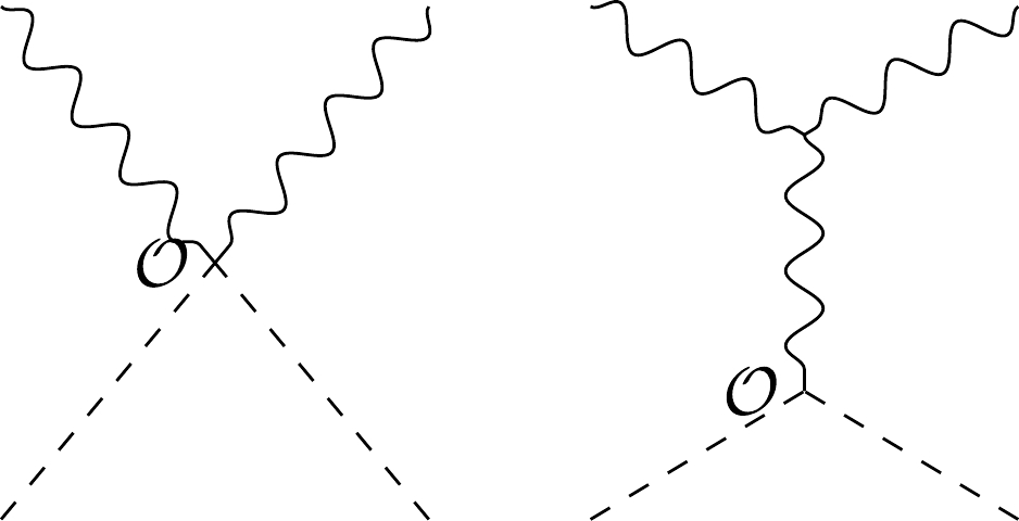
Figure C1. Two Feynman diagrams that contribute to
$W^{a,+}\pi^b \to $ $ W^{a,+}\pi^b$ from effective operators.In terms of our amplitude basis, this conclusion can be considerably simplified without any cancelation in Fig. C1. The elastic scattering process is of type
$ f(F^-F^+\phi^2) $ , whose primary amplitude is$ [2|p_3| {1} \rangle^2 $ , which is of dimension$ 8 $ . Moreover, on-shell amplitudes cannot be constructed recursively from$ d=6 $ ; hence, no overall on-shell contribution is provided by dimension 6 operators.
Standard model effective field theory from on-shell amplitudes
- Received Date: 2022-10-24
- Available Online: 2023-02-15
Abstract: We present a general method of constructing unfactorizable on-shell amplitudes (amplitude basis) and build up their one-to-one correspondence to the independent and complete operator basis in effective field theory (EFT). We apply our method to the Standard Model EFT and identify the amplitude basis in dimensions 5 and 6, which correspond to the Weinberg operator and operators in the Warsaw basis, except for some linear combinations.


 DownLoad: