


 Abstract
 HTML
HTML Reference
 Related
 PDF
PDF


-
In 2019, the Event Horizon Telescope (EHT) Collaboration produced the iconic image of the black hole residing at the center of the elliptical galaxy Messier 87*. Essential optical features of the image, such as the black hole shadow first investigated by Bardeen et al. [1, 2], are entirely governed by intrinsic black hole parameters, such as the mass, charge, and angular momentum. Therefore, this achievement of the EHT Collaboration strongly indicates a promising means of probing gravity in the strong-field regime. That is, observations are performed in terms of the electromagnetic signals, in addition to those through gravitational waves. In this regard, the black hole shadow is a relevant topic that is essential to our understanding of the properties of black holes and the geometric structure of the relevant spacetime. With further improvement in the resolution in future, observation of the shadow is expected to provide us with direct access to the geometrical characteristics of compact objects [3]. Moreover, it might become feasible for the extracted information on the properties of spacetime geometry to be utilized to discriminate between different candidate theories of gravity.
In the past decades, many scenarios of modified gravity have been proposed and extensively studied, aiming at various theoretical and observational problems that cannot be straightforwardly answered in the framework of general relativity. The black hole no-hair theorem states that in Einstein-Maxwell theory, an isolated black hole is characterized by its mass, electric charge, and angular momentum, while the condensation of other non-trivial matter fields is not possible [4–7]. Ever since the idea was proposed by Wheeler, it has attracted continuous attention over several decades. The notion of the no-hair theorem has also been extended to alternative theories of gravity, such as Brans-Dicke theory, the scalar tensor theories [8–18], and their generalization, the Horndeski gravity [3, 19]. Beyond the framework of Einstein-Maxwell theory, many counter-examples to the no-hair theorem have been established. For instance, black hole solutions have been encountered with Skyrme, dilaton, or Yang-Mills-Higgs hair. Furthermore, in the so-called spontaneous scalarization, non-minimal coupling between a scalar field and either the Maxwell invariant, Gauss-bonnet term, or Ricci scalar gives rise to scalar hairy black hole solutions [20–28].
On the theoretical side, the shadow of a celestial body can be evaluated by studying a particular type of null geodesic known as fundamental photon orbits [29, 30]. The boundary of a black hole shadow, in turn, is governed mainly by unstable photon orbits, which might lead to novel features, such as cuspy [29, 31], open [32], or fractured [31] black hole silhouettes. Recently, this concept has been explored in the context of nonlinear electrodynamics (NLED). Owing to substantial implications in modern material science, excitement in NLED was rekindled, and its development has been closely associated with the maturity of quantum electrodynamics. Existing photon-photon scattering experiments strongly indicate that electrodynamics may be nonlinear in vacuum [33–35]. When compared to linear Maxwell electrodynamics, the different behavior of the photons in an NLED environment is revealed via intriguing properties. In particular, field perturbation does not propagate along the null geodesic of the background geometry. However, it was shown by Novello et al. that the normal vector of a finite discontinuity follows the null geodesic of an effective geometry [36]. As a null vector in the effective metric, the propagation vector of the discontinuity can be viewed as that of a photon. The latter is feasible because the classical notion of a photon's geodesic can be established by approximating the perturbation equation of the electromagnetic field at the geometric-optics limit [37–39]. More specifically, at the lowest order, the propagation vector of the waveform manifestly follows the trajectory of a null geodesic. Subsequently, regarding the black hole shadow, the above intriguing result provides a theoretical basis for studying fundamental photon orbits in black holes associated with NLED.
The present study involves an attempt to investigate the properties of the black hole shadow in square-root
$ f(R) $ gravity containing photons when the electromagnetic fields are nonlinear. In particular, we explore the rotating counterpart based on a static black hole solution first obtained in Ref. [19]. The effective metric is derived in which the photons propagate, and the resulting black hole shadows are investigated. This paper is structured as follows. In the next section, we elaborate on the rotating black hole solution and the effective geometric metric for the photons of NLED. In Sec. III, we obtain the image of the black hole and its shadow and subsequently analyze its properties concerning the relevant model parameters. Sec. IV is devoted to further discussions and concluding remarks. -
In this section, we elaborate on the rotating black hole in question in
$ f(R) $ gravity and derive the effective metric. The rotating black hole solution is obtained based on the static black hole solutions given in [19]. The action that describes NLED in$ f(R) $ gravity is expressed as$ S=\frac{1}{2}\int\sqrt{-g}f(R){\rm d}^4{x}+\int\sqrt{-g}L(F){\rm d}^4{x}, $

(1) where R is the Ricci scalar. For this study, we focus on the square-root theory
$ f(R)=R-2\alpha \sqrt{R} $ , where α is a coupling constant.$ L(F) $ is the Lagrangian of the nonlinear electromagnetic field. We consider a specific form of the electromagnetic field, given by [19]$ L(F)=\frac{c_3^{2}}{c_1}F+\frac{c_3}{\sqrt{c_1}}\sqrt{F} c_4+c_{1}c_4^{2}, $

(2) where
$ F=\dfrac{1}{4}F_{\mu\nu}F^{\mu\nu} $ , and the parameters$ c_1,c_3 $ , and$ c_4 $ are constants. The physical meaning of these metric parameters are further elaborated on below regarding the spherical solutions to the action in Eq. (1). Note that the first term in Eq. (2) is proportional to the Maxwell action, whereas the second term gives a non-linear correction. As$ c_4 $ vanishes, Eq. (2) returns to standard linear Maxwell electromagnetism.A spherical solution to this model was obtained in [19]. The resultant metric has the form
$ {\rm d}s^2=-H(r){\rm d}t^2+\frac{{\rm d}r^2}{H(r)}+r^2({\rm d}{\theta}^2+{\rm sin}^2{\theta}{\rm d}{\phi}^2), $

(3) $ H(r)=\frac{c}{2}-\frac{2M}{r}+\frac{q^2}{r^2}. $

(4) Here,
$ M=-\dfrac{c_1}{2} $ is related to the black hole mass, and the parameter q corresponds to the electric charge. The parameter c satisfies$ 0<c<2 $ , which is taken to be the unit in this study. The electromagnetic potential, defined as one-form, is given by$ \begin{array}{*{20}{l}} V_1=p(r){\rm d}t+n(\phi){\rm d}r+s(r){\rm d}\phi, \end{array} $

(5) where
$ p(r)=\dfrac{c_3}{r} $ ,$ n(\phi)= c_4{\phi} $ , and$ s(r)=c_4{r} $ are associated with the electric and magnetic charges that govern the potential.The rotating metric solution of Eq. (1) can be obtatined by applying a transformation [40, 41] to the spherical static metric in Eq. (3),
$ \begin{aligned}[b] \overline{\phi}=&\Xi\phi+\omega t,\\ \overline{t}=&\Xi{t}+\omega\phi, \end{aligned} $

(6) where ω is the rotation parameter, and
$ \Xi=\sqrt{1+{\omega}^2} $ . The resultant rotating solution is$ \begin{aligned}[b] {\rm d}s^2=&[{\Xi}^{2}H-{\omega}^{2}r^2{\rm sin}^2{\theta}]{\rm d}t^2-\frac{{\rm d}r^2}{H}-r^2{\rm d}{\theta}^2\\ &-[{\Xi}^2r^2{\rm sin}^2{\theta}-{\omega}^2H]{\rm d}{\phi}^2+2\omega\Xi[H-r^2{\rm sin}^2{\theta}]{\rm d}t{\rm d}\phi\nonumber , \end{aligned} $

and the electromagnetic potential reads as
$ \begin{array}{*{20}{l}} { } V_2={[\Xi{p(r)}+\omega{s(r)}]}{\rm d}t+c_4{(\Xi\phi+\omega{t})}{\rm d}r+{[\omega{p(r)+\Xi{s(r)}}]}{\rm d}\phi . \end{array} $

(7) As the rotating parameter ω vanishes, Eq. (7) returns to the static solution in Eq. (3). It is also worth mentioning that [40] the two solutions Eqs. (3) and (7) are locally, but not globally, mapped onto each other. The non-vanishing components of field strength are
$ F_{tr}=\frac{\Xi c_3}{r^2}=-F_{rt},~~ F_{\phi r}=\frac{c_3 \omega}{r^2}=- F_{r\phi}. $

(8) -
As mentioned before, in spacetime with nonlinear electromagnetic fields, the trajectory of a photon is different from that in Maxwell fields. Instead of the null geodesics of background spacetime, the motion of the photon is governed by the null geodesics of an effective geometry [36]. Next, we study geodesic motion in the background of the charged rotating black hole, Eq. (7). Using the method established in [36], we evaluate the effective metric in the presence of nonlinear electromagnetic fields. Calculations of the null geodesics and resultant black hole image are performed in the following sections. According to [36], a finite discontinuity is present along the normal direction of a surface in its first derivative. The norm of the surface
$ k^{\mu} $ , identified to be the propagation vector of a photon, is found to satisfy$ (L_{F}\tilde{g}^{\mu\nu}-4L_{FF}F^{\mu\alpha}F_{\alpha}^{\nu})k_{\mu}k_{\nu}=0 , $

(9) where
$ \tilde{g}^{\mu\nu} $ is the metric of spacetime, and$ L_F $ and$ L_{FF} $ denote the first and second derivatives of$ L(F) $ with respect to F, respectively. From Eq. (10), we can readily extract an effective spacetime metric$ g^{\mu\nu} $ (without a "hat") that reads as$ \begin{array}{*{20}{l}} { } g^{\mu\nu}=L_F \tilde{g}^{\mu\nu}-4L_{FF}F^{\mu}_{\alpha}F^{\alpha\nu} , \end{array} $

(10) and it can be further shown that the norm transports itself parallelly in the effective metric, or in other words, the photon propagates along the null geodesics. When the nonlinear coupling parameter
$ c_4 $ vanishes, Eq. (2) simplifies to the form$ L(F)=\frac{c_3^{2}}{c_1}F $ , and NLED reduces to Maxwell theory. When$ L_F $ is a constant, as$ L_{FF} $ vanishes, the effective metric in Eq. (10) returns to that of the background, Eq. (7).Using Eqs. (7), (8), and (10), we obtain an expression for the effective metric,
$ \begin{array}{*{20}{l}} {\rm d}s^2=g_{tt}{\rm d}t^2+g_{rr}{\rm d}r^2+g_{\theta\theta}{\rm d}{\theta}^2+g_{\phi\phi}{\rm d}{\phi}^2+2g_{t\phi}{\rm d}t{\rm d}{\phi} , \end{array} $

(11) where the components are
$ \begin{aligned}[b]\\[-8pt] {g}_{tt}=&\frac{2H(1+\omega^2)(-M+c_4M^{\frac{3}{2}}r^2)+2\omega^2r^2{\rm sin}^2{\theta}(M+3c_4M^{\frac{3}{2}}r^2)}{1+2c_4\sqrt{M}r^2-3Mc_4^2r^4} ,\\ {g}_{rr}=&\frac{2M}{H(1+3c_4\sqrt{M}r^2)} ,\\ {g}_{\theta\theta}=&\frac{2Mr^2}{1-c_4\sqrt{M}r^2} ,\\ {g}_{\phi\phi}=&\frac{2H\omega^2(-M+c_4M^{\frac{3}{2}}r^2)+2(1+\omega^2)r^2{\rm sin}^2{\theta}(M+3c_4M^{\frac{3}{2}}r^2)}{1+2c_4\sqrt{M}r^2-3Mc_4^2r^4} ,\\ {g}_{t\phi}=&\frac{2H\omega\sqrt{1+\omega^2}(-M+c_4M^{\frac{3}{2}}r^2)+2\omega\sqrt{1+\omega^2}r^2{\rm sin}^2{\theta}(M+3c_4M^{\frac{3}{2}}r^2)}{1+2c_4\sqrt{M}r^2-3Mc_4^2r^4} . \end{aligned} $ 
(12) The horizons of the effective metric in Eq. (11) are determined by solving
$ g_{rr}^{-1}=0 $ , which gives$ \begin{array}{*{20}{l}} r_h=2M\pm\sqrt{4M^2-2q^2} . \end{array} $

(13) Note that the radii have no relevance to the nonlinear coupling
$ c_4 $ because they are entirely determined by$ H(r) $ . The radius in Eq. (13) is only related to the propagation of discontinuity but not necessarily to other types of perturbations. Moreover, it has nothing to do with the nonlinear coupling$ c_4 $ because it is entirely determined by$ H(r) $ . Hereafter, the word "horizon" refers to the quanta originating from the electromagnetic perturbations and therefore light rings and black hole shadows. -
Employing the reverse ray-tracing method [42, 43], we investigate the shadow of the rotating charged black hole described by Eq. (7).
To solve the trajectories of the photon, we start with the Lagrangian
$ L=\frac{1}{2}g_{\mu\nu}\dot{x}^{\mu}\dot{x}^{\nu}=0 , $

(14) where the dots denote the derivatives with respect to the affine parameter. The resultant equations that describe the null geodesics are expressed as
$ \begin{aligned}[b] \ddot{r}=&\frac{1}{2}\Bigg[\left(\frac{\partial{g_{tt}}}{\partial{r}}\right)\dot{t}^2+2\left(\frac{\partial{g_{t\phi}}}{\partial{r}}\right)\dot{t}\dot{\phi}+\left(\frac{\partial{g_{\phi\phi}}}{\partial{r}}\right)\dot{\phi}^2-\left(\frac{\partial{g_{rr}}}{\partial{r}}\right)\dot{t}^2\\&-2\left(\frac{\partial{g_{rr}}}{\partial{\theta}}\right)\dot{r}\dot{\theta}+\left(\frac{\partial{g_{\theta\theta}}}{\partial{r}}\right)\dot{\theta}^2\Bigg] ,\\ \ddot{\theta}=&\frac{1}{2}\Bigg[\left(\frac{\partial{g_{tt}}}{\partial{\theta}}\right)\dot{t}^2+2\left(\frac{\partial{g_{t\phi}}}{\partial{\theta}}\right)\dot{t}\dot{\phi}+\left(\frac{\partial{g_{\phi\phi}}}{\partial{\theta}}\right)\dot{\phi}^2\\&+\left(\frac{\partial{g_{rr}}}{\partial{\theta}}\right)\dot{r}^2-2\left(\frac{\partial{g_{\theta\theta}}}{\partial{r}}\right)\dot{r}\dot{\theta}-\left(\frac{\partial{g_{\theta\theta}}}{\partial{\theta}}\right)\dot{\theta}^2\Bigg] , \end{aligned} $

(15) where
$ \begin{aligned}[b] \dot{t} =& \frac{Eg_{\phi\phi}+L_{z}g_{t\phi}}{g_{t\phi}^2-g_{tt}g_{\phi\phi}} ,\\ \dot{\phi}= &\frac{Eg_{t\phi}+L_{z}g_{tt}}{g_{tt}g_{\phi\phi}-g_{t\phi}^2} . \end{aligned} $

The effective metric Eq. (10) possesses two killing vectors,
$ \zeta_t $ and$ \zeta_{\phi} $ , implied by the axisymmetry. Two constants of motion are generated for a free falling particle moving along the geodesic, corresponding to the energy E and the$ z- $ component of the angular momentum$ L_z $ . We have$ E=-P_t=-\partial{L}/\partial{\dot{t}} $ and$ L_z=P_{\phi}=\partial{L}/\partial{\dot{\phi}} $ .In our calculations, we assume that a stationary observer is locally at (
$ r_\mathrm{obs} $ ,$ \theta_\mathrm{obs} $ ) with a vanishing angular momentum. We consider an orthornormal basis, ($ {e_{\hat{t}}} $ ,$ {e_{\hat{r}}} $ ,$ {e_{\hat{\theta}}} $ ,$ {e_{\hat{\phi}}} $ ), in the observer's local frame of reference, which is related to the coordinate basis ($ \partial_{t} $ ,$ \partial_{r} $ ,$ \partial_{\theta} $ ,$ \partial_{\phi} $ ) by$ {e_{\hat{\mu}}}={e_{\hat{\mu}}^{\nu}}\partial_{\nu} $ via a transform matrix,$ {e_{\hat{\mu}}^{\nu}} $ , that satisfies$ g_{\mu\nu}{e_{\hat{\alpha}}^{\nu}}{e_{\hat{\beta}}^{\nu}}=\eta_{\hat{\alpha}\hat{\beta}} $ , where$ \eta_{\hat{\alpha}\hat{\beta}} $ is the metric of Minkowski spacetime. Because the transformation matrix is not unique up to the Lorentz transformation, we choose the following form:$ \begin{array}{*{20}{l}} {e_{\hat{\mu}}^{\nu}}= \left[{\begin{array}{cccc} \zeta&0&0&\gamma\\ 0&A^r&0&0\\ 0&0&A^{\theta}&0\\ 0&0&0&A^{\phi}\\ \end{array}}\right] , \end{array} $

(16) where ζ,
$ A^{r} $ , γ,$ A^{\theta} $ , and$ A^{\phi} $ are real coefficients. By considering the normalization$ {e_{\hat{\mu}}}{e^{\hat{\nu}}}={\delta_{\hat{\mu}}}^{\hat{\nu}} $ , we get$ \begin{aligned}[b] A^r=&\frac{1}{\sqrt{g_{rr}}},\quad A^{\theta}=\frac{1}{\sqrt{g_{\theta\theta}}},\quad A^{\phi}=\frac{1}{\sqrt{g_{\phi\phi}}},\\ {\zeta}=&\sqrt{\frac{g_{\phi\phi}}{g_{t \phi}^2-g_{tt} g_{\phi\phi}}},\quad \gamma=-\frac{g_{t \phi}}{g_{\phi\phi}}\sqrt{\frac{g_{\phi\phi}}{g_{t \phi}^2-g_{tt} g_{\phi\phi}}}. \end{aligned} $

The locally measured four-momentum
$ p^{\hat{\mu}} $ can be expressed by the projection of its four-momentum in$ p^{\mu} $ onto the observer's basis,$ \begin{array}{*{20}{l}} p^{\hat{t}}=-p_{\hat{t}}=-{e_{\hat{t}}}^{\nu}p_{\nu},\; p^{\hat{i}}=p_{\hat{i}}={e_{\hat{i}}}^{\nu}p_{\nu} , \end{array} $

(17) where the components are
$ p^{\hat{t}}=\zeta E-\gamma L,\; p^{\hat{r}}=\frac{1}{\sqrt{g_{rr}}}p_r,\; p^{\hat{\theta}}=\frac{1}{\sqrt{g_{\theta\theta}}}p_\theta,\; p^{\hat{\phi}}=\frac{1}{\sqrt{g_{\phi\phi}}}L. $

In the observer's sky, the coordinates
$ (x,\; y) $ assigned to each photon are expressed as [44]$ x=-r\frac{p^{\hat{\phi}}}{p^{\hat{r}}}\mid_{(r_\mathrm{obs},\theta_\mathrm{obs})},y=r\frac{p^{\hat{\theta}}}{p^{\hat{r}}}\mid_{(r_\mathrm{obs},\theta_\mathrm{obs})}. $

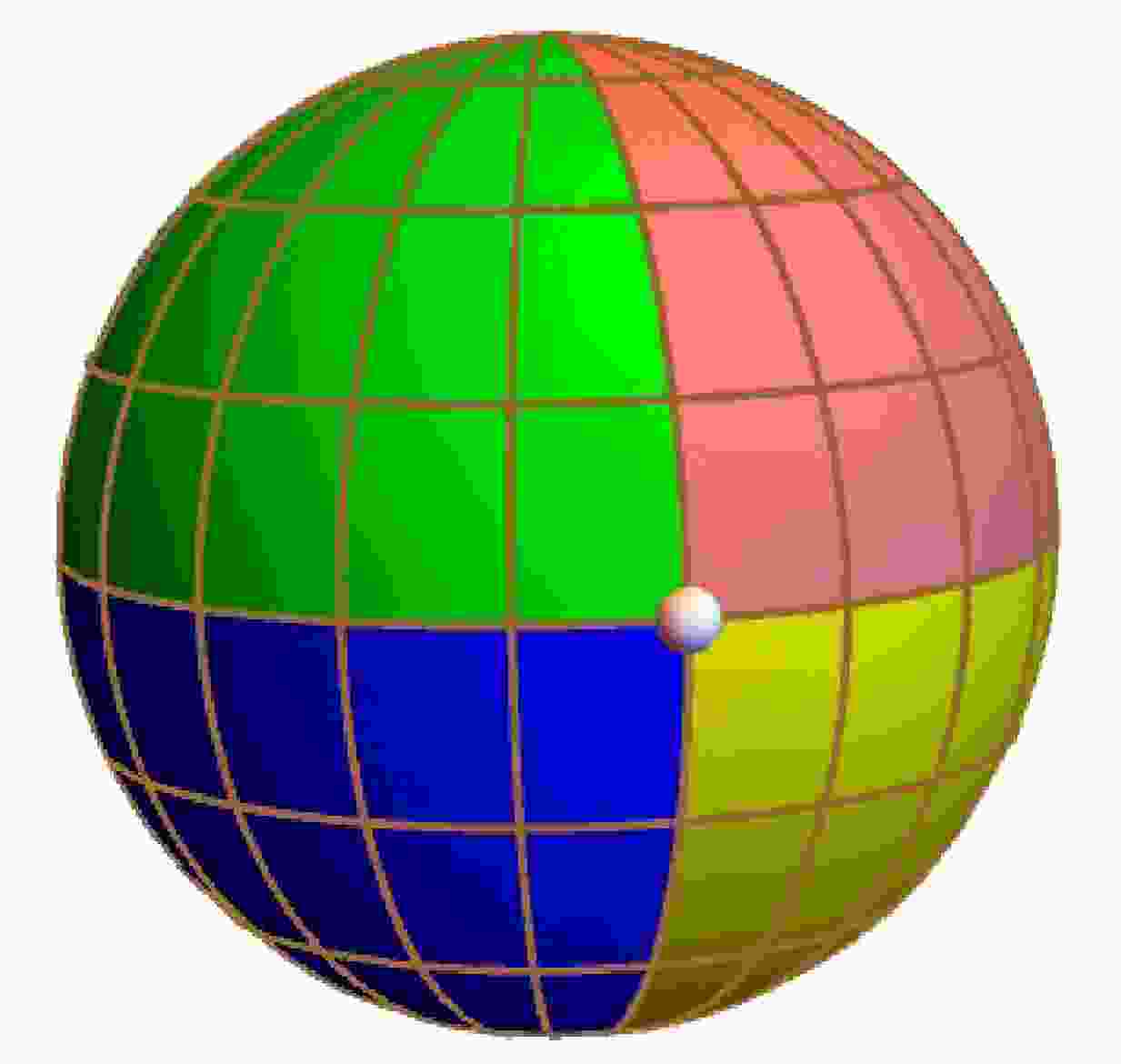
(18) The celestial sphere is divided into four quadrants marked with distinct colors [42,43, 45–49], green, blue, red, and yellow, as shown in Fig. 1.
Figure 1. (color online) Panoramic view of the celestial sphere.
A grid of longitude and latitude lines is marked with adjacent brown lines separated by
$ {10}^{\circ} $ . The observer is placed at the intersection of the four colored quadrants, with$r_\mathrm{obs}=r_{\rm sphere}$ , oriented toward the origin. For convenience, the observer is not shown in Fig. 1. The observer's local sky is divided into many small solid angles, and each corresponds to a pixel in the final image. We follow the trajectory of each photon associated with a pixel's viewing angle by numerically integrating Eq. (15) until they either reach a point on the celestial sphere or hit the black hole horizon. If the photon falls into the horizon, it is counted as a black pixel located inside the shadow. If it hits the celestial sphere, the asymptotic angular direction of the photon is used to identify one of the four colors that is subsequently assigned to a pixel in the resultant image. However, its coordinates are governed by the photon's initial solid angle. An image of the black hole is eventually constructed by enumerating the solid angles in the observer's local sky. In our study, we choose$ r_\mathrm{obs} = 50M $ and the inclination$ \theta_\mathrm{obs} = 90^{\circ} $ . Following the practice of other authors [43,45–49], a white reference point is placed at the other intersection of the four colored quadrants. In a spherically symmetric black hole metric, the latter eventually gives rise to the Einstein ring(s) shown in the observer's sky. -
This section explores the effects of the black hole spin parameter ω on the resultant shadows. Calculations are performed for the given nonlinear coupling parameter
$ {c_4}=1 $ and charge$ q=1 $ , but with different spin parameters. The resultant images of the black hole are given in Fig. 2. In the resultant images, the white arc structures located outside the black hole shadow correspond to the lowest order Einstein arc or ring, particularly when it forms a complete circle. The region within the Einstein ring corresponds to the photons whose trajectories circulate the black hole for more than one complete circle, and an infinite number of images are produced. Among them, the most visible one corresponds to an inverted image of the celestial sphere, because the color of the corresponding regions of the image is manifestly reflected. This demonstrates severe aberration due to strong gravitational lensing, which corresponds to the singularities in the lensmaker's equation. As an essential optical feature, it can also be used to extract information on mass distribution. Hereafter, unless otherwise stated, the above configuration is utilized throughout the numerical study.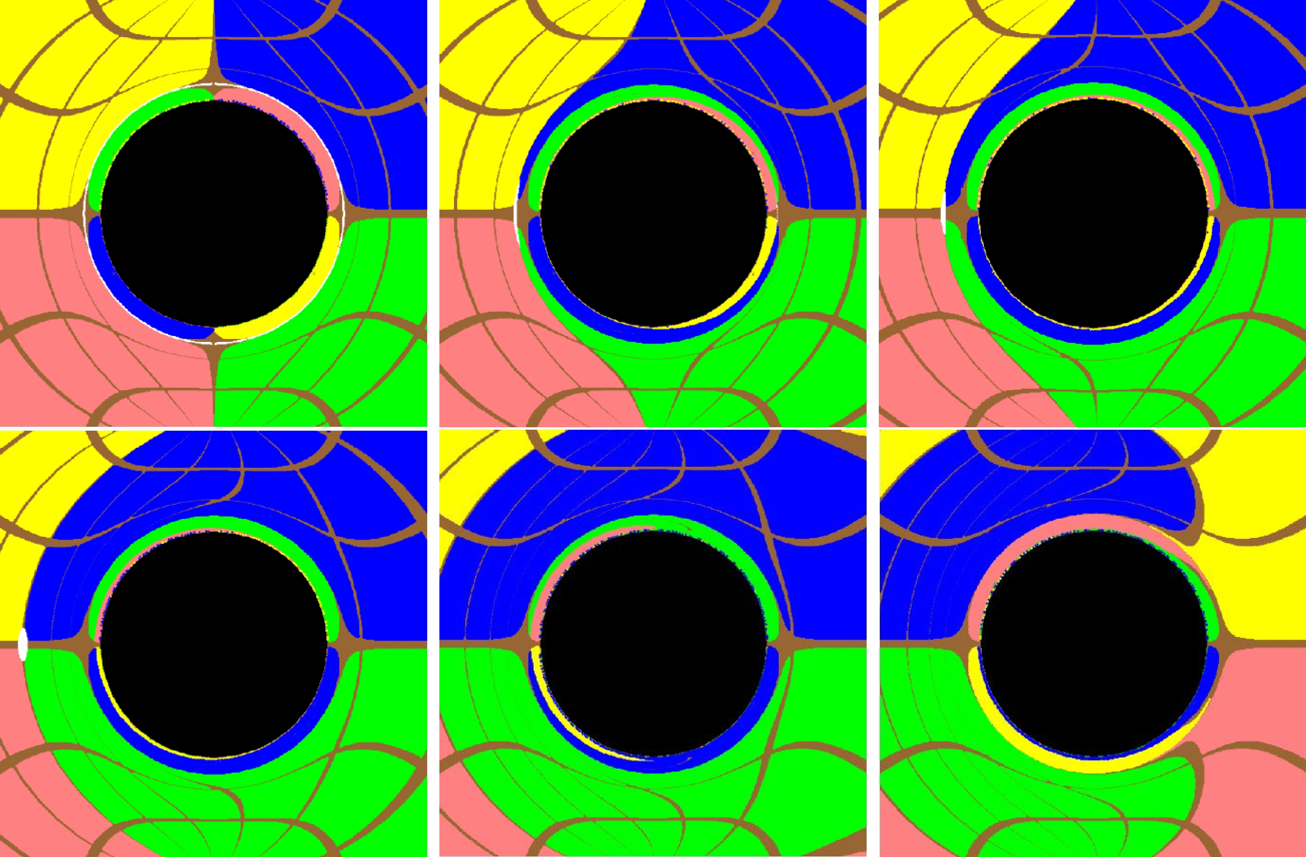
Figure 2. (color online) Images of the black hole obtained for different spins
$ {\omega} $ with the given metric parameters$M=3,~ q=1,~ c_4=1$ . For the upper row, from left to right, the plots are evaluated using${\omega}=0, 0.001,~ 0.002$ , whereas for the bottom row, from left to right, the plots are evaluated using${\omega}=0.005,~ 0.007,~ 0.009$ . The colors (red, yellow, blue, and green) in the image are those of the four quadrants of the celestial sphere. The black part at the center of the image is the shadow of the black hole.In the top-left plot of Fig. 2, we consider the case
$ \omega=0 $ , which corresponds to the case of the static spherically symmetric black hole solution. Here, a complete Einstein ring shown in white is visible. In this case, gravitational lensing is isotropic. By gradually increasing the value of$ {\omega} $ , the remaining plots give the corresponding images of the rotating black hole.It is observed that the black hole's spin has a frame-dragging effect on spacetime, which pulls space in the direction of the black hole's rotation. Besides the shape of the regions with different colors, the warping direction of the brown curve and the warping degree of the four-color regions are also observed. These plots visually present how the black hole's spacetime is deformed owing to the frame-dragging of the stationary metric. In particular, in Fig. 2, the spin axis of the black hole points upward, and subsequently, space is twisted and spans from right to left. As one gets closer to the black hole, the frame-dragging becomes stronger. This can be inferred from the degree of deformation of the brown lines in the background grid. Additionally, as the black hole's spin breaks the spherical symmetry of spacetime, it causes different lensing effects in different directions of the observer's local sky. This is shown by the shifted position and distortion of the white Einstein ring. Moreover, it can be seen from the comparison between different spin values that the frame-dragging effect becomes more evident with increasing spin. In contrast, the black hole shadow is not sensitive to the spin, because the size of the central black hole shadow mostly remains unchanged, as shown in Fig. 2.
-
In this subsection, we study the role of the coupling parameter
$ c_4 $ in the resulting black hole images. In our calculations, we choose the metric parameters$ {\omega}=0.003 $ ,$ q=1 $ , and$ M=3 $ , while varying$ c_4 $ . As observed in Fig. 3, the impact of the change on the resultant black hole shadow is significant in two aspects. First, in the plots on the first row of Fig. 3, as the coupling increases from$ 0.005 $ to$ 1 $ , the size of the black hole shadow decreases. Meanwhile, the frame-dragging of the rotating black hole does not seem to depend on the coupling, because the spacetime distortion remains unchanged. Second, as the coupling further increases, the gravitational lensing and size of the black hole shadow converges to a given value. This is demonstrated in the second row of Fig. 3, where the coupling varies from$ 9 $ to$ 1000 $ . Overall, the four plots are mainly identical. Such a saturation phenomenon might be an interesting feature of the model.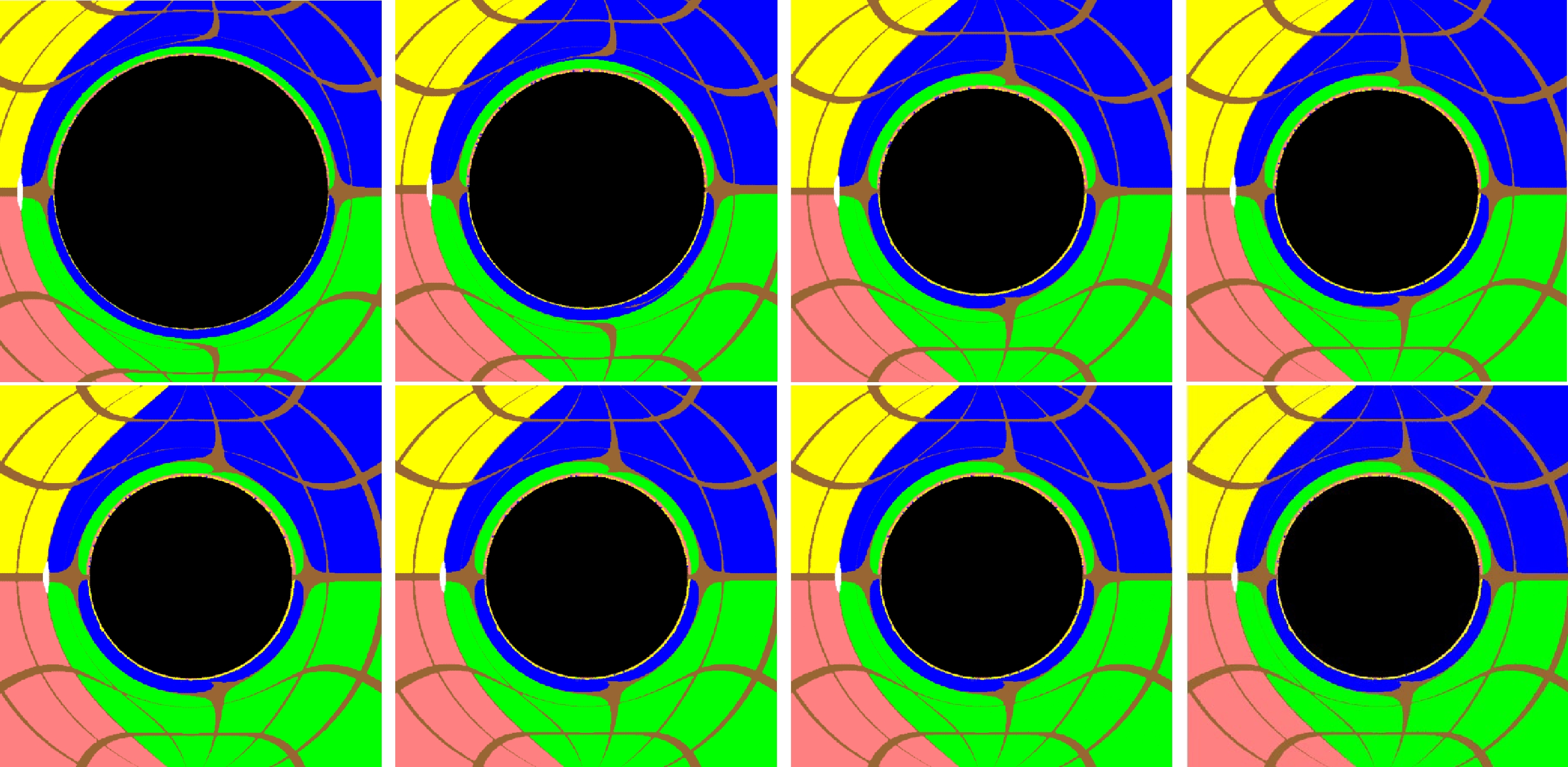
Figure 3. (color online) Images of the black hole obtained for different coupling parameters
$ c_4 $ with the given metric parameters$M=3,~ q=1,~ \omega=0.003$ . For the upper row, from left to right, the plots are evaluated using$c_4 = 0.005,~ 0.01,~ 0.1,~ 1$ , whereas for the bottom row, from left to right, the plots are evaluated using${c_4}=9,~50,~100,~1000$ . The remaining conventions are the same as in Fig. 2.Here, to analyze the characteristics of the black hole shadow in detail, we introduce the shadow's average radius
$ R_s $ using the following expression [50, 51]:$ R_s=\frac{({b_1}-{d_1})^2+{b_2}^2}{2|{b_1}-{d_1}|} , $

(19) where
$ R_s $ is the radius of the reference circle defined as passing through three points:$ B(b_1,b_2) $ as the top point,$ C(c_1,c_2) $ as the bottom point, and$ D(d_1,d_2) $ as the right point.In Fig. 4, we show the shadow radius
$ R_s $ as a function of the nonlinear coupling parameter$ c_4 $ . The shadow radius$ R_s $ is shown to be sensitive to the nonlinear coupling parameter$ c_4 $ when$ c_4 < 0.1 $ and increases with increasing$ c_4 $ . It converges to a particular value as$ c_4 $ increases further. This is consistent with what is observed in the black hole image.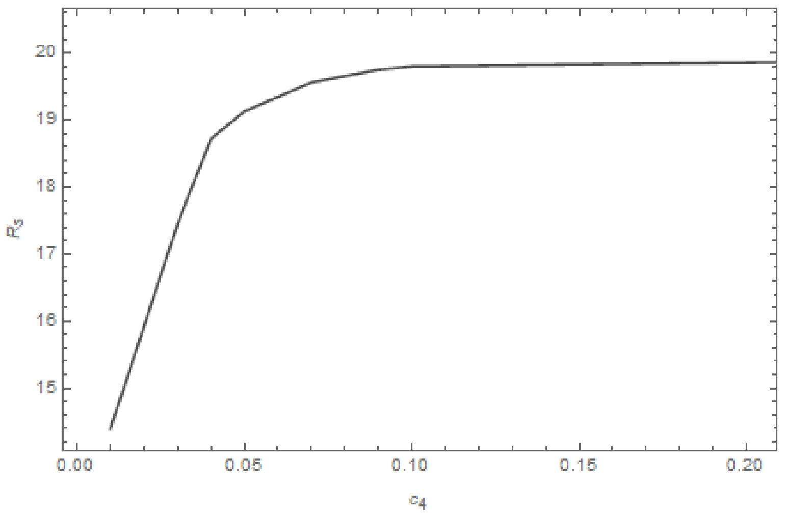
Figure 4. Obtained shadow radius
$ R_s $ as a function of the nonlinear coupling parameter$ c_4 $ . -
Finally, we explore the effect of the black hole's charge. Calculations are performed using given metric parameters of
$ M=3 $ ,$ \omega=0.003 $ , and$ c_4=1 $ while varying the charge q of the black hole. As shown in Fig. 5, the charge does not have a significant impact on frame-dragging. However, the size of the black hole shadow decreases as the charge increases. This is a somewhat expected feature owing to the relationship between the outer horizon radius and charge given in Eq. (13), reminiscent of the case of Reissner-Nordström black holes.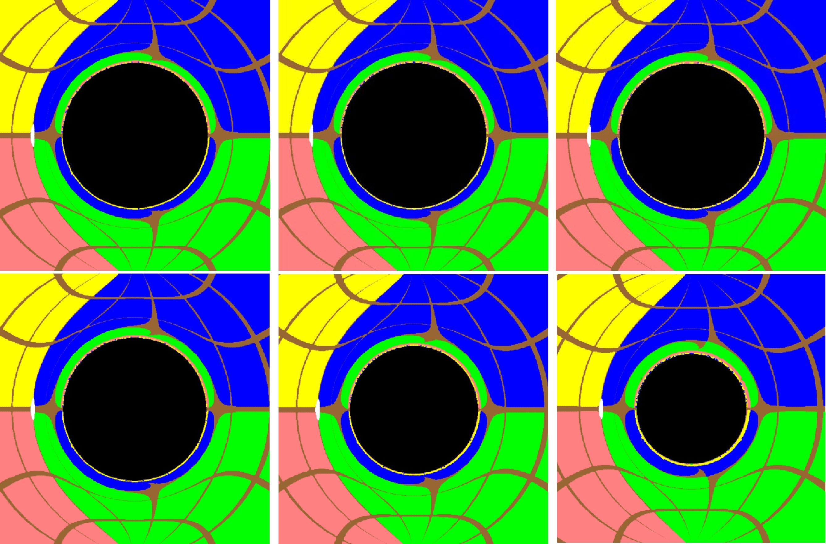
Figure 5. (color online) Images of the black hole obtained for different coupling parameters q with the given metric parameters
$M=3,~ c_4=1,~ \omega=0.003$ . For the upper row, from left to right, the plots are evaluated using$q = 0.005,~ 0.3,~ 0.5$ , whereas for the bottom row, from left to right, the plots are evaluated using$q=1,~ 3,~ 4$ . The remaining conventions are the same as in Fig. 2.Similarly, we plot the shadow radius
$ R_s $ as a function of the black hole's charge q. In Fig. 6, we find that the radius decreases monotonically with increasing charge, which is consistent with the black hole's image. This indicates that one might extract information on the charge if specific parameters of an astrophysical system are provided, such as in the case of [50].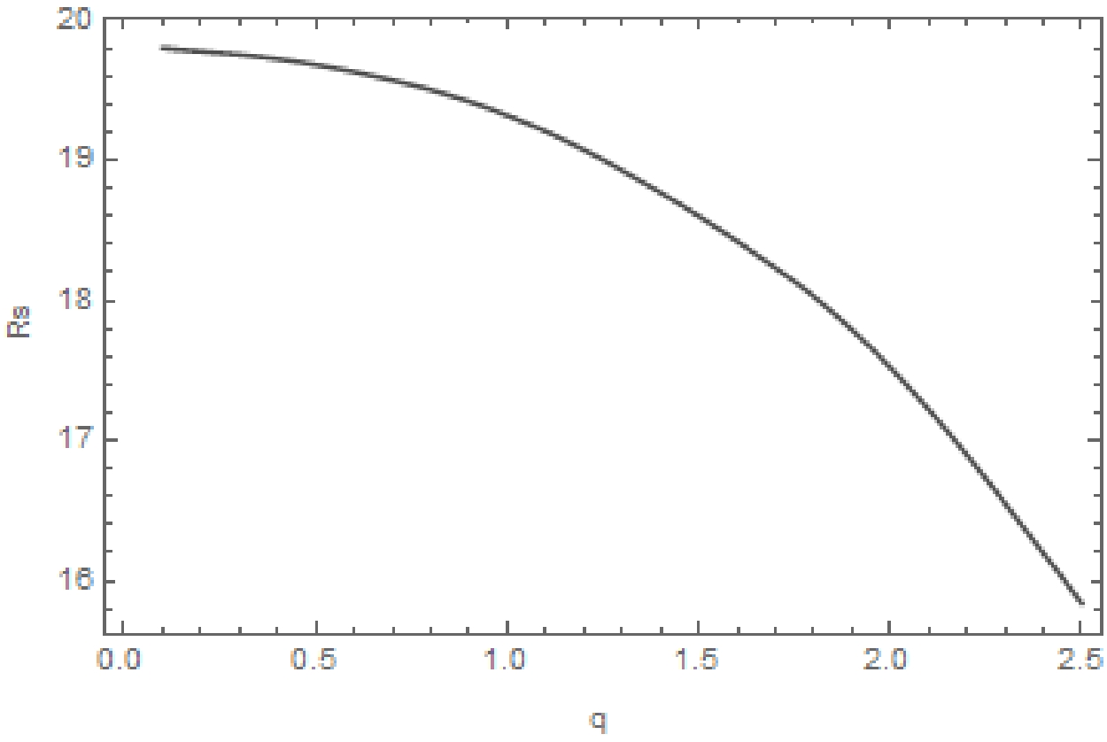
Figure 6. Obtained shadow radius
$ R_s $ as a function of the black hole charge q. -
In this study, we investigate the images of a charged black hole in nonlinear Maxwell
$ f(R) $ gravity. We obtain the effective geometric metric for photons propagating in the nonlinear medium. Using the inverse ray-tracing method, the photon trajectories are calculated, and the black hole shadow images are obtained. We explore the effects of relevant metric parameters, namely the spin, charge, and nonlinear coupling parameters, on the resultant black hole shadow. As the black hole spin increases, frame-dragging becomes more significant, whereas the overall size of the shadow is found to be less sensitive to spin. In contrast, the effect of frame-dragging does not significantly depend on either the charge or the nonlinear coupling parameter. With a more significant charge, the outer horizon of the black hole becomes smaller. Subsequently, the size of the shadow also decreases, in accordance with the case of Reissner-Nordström black holes. While the horizon of the black hole is not a function of the nonlinear coupling parameter, the size of the black hole shadow is found to decrease with increasing coupling. Moreover, after the coupling reaches a threshold value, the black hole shadow converges to a specific size independent of the coupling parameter.
Black hole shadow in f(R) gravity with nonlinear electrodynamics
- Received Date: 2022-08-19
- Available Online: 2023-02-15
Abstract: By analyzing the propagation of discontinuity in nonlinear electrodynamics, we numerically investigate the related black hole shadows of recently derived rotating black hole solutions in


 DownLoad: