Isoscalar monopole strength in ¹⁰⁰Mo: an indicator for static triaxial deformation in the ground state

I. INTRODUCTION

• I. INTRODUCTION
• II. MODEL
• III. RESULTS AND DISCUSSIONS
•      A Ground state potential-energy surfaces
•      B ISM strength functions
•      C Coupling between isoscalar quadrupole andmonopole vibrations
• IV. SUMMARY
• ACKNOWLEDGMENTS

Recent years have seen renewed interest in compression-mode resonances, such as the isoscalar giant resonances in nuclear physics [1]. From the resonance energy, it is possible to extract the incompressibility of uniform nuclear matter, which is an important parameter of the equation of state.

In nuclear density functional theories (DFTs), nuclear matter properties including the incompressibility parameter at saturation, $K_{\infty}$, can be derived from the functional [2]. Consequently, it is customary to take an energy-density functional (EDF) that successfully describes the properties of finite nuclei and examine its performance when applied to the description of compression-mode resonances. If the theory can simultaneously account for the ground-state data and observed resonance energies, the incompressibility offered by the EDF is considered reliable.

Although progress has been made [3], several issues remain. For example, most EDFs systematically overestimate the isoscalar giant monopole resonance energies of tin isotopes [4]. This is curious because the same EDFs can reproduce the ground state observables as well as the resonance energies in other nuclei, such as $^{90}$Zr and $^{208}$Pb [5]. This suggests that structural properties depending on isospin become important in describing the isoscalar monopole (ISM) mode. To obtain a better model and an accurate incompressibility parameter, it is desirable to expand our knowledge of ISM vibration in other nuclei.

Recently, the strengths of the ISM vibration mode were systematically observed in $^{90}$Zr and $^{92,94,96,98,100}$Mo nuclei [6, 7]. Focusing on the Mo isotopes, for $^{92,94,96,98}$Mo, the observed strengths as a function of excitation energy exhibit generic single broad peaks in the interval of $16 < E<17$ MeV. From $^{94}$Mo, a lower-energy shoulder emerges at $E\approx13$ MeV and becomes more pronounced in $^{96,98}$Mo. For ¹⁰⁰Mo, the structure of the strength function reveals a multi-peak feature.

While the strengths in the lighter Mo isotopes ($N<58$) seem to be based on spherical or weak deformation, the strength function of ¹⁰⁰Mo may indicate large static triaxial deformation in the ground state. Indeed, it has been known that neutron-rich Mo isotopes manifest a variety of interesting shape evolutions as a function of angular momentum and isospin [8]. In particular, the neutron-rich Mo and Ru nuclei have long been calculated to have triaxial ground states. A definitive signature of triaxial deformation in the ground state of the nucleus has been rather scarce. Experimental confirmation of axial symmetry breaking will have far-reaching consequences [9].

In this study, we calculate the strength of the ISM vibration mode by constraining the ground state to several typical deformations. The resulting strength functions are compared with the experimental data. This approach may allow for a quantitative determination of static triaxial deformation in the ground state of ¹⁰⁰Mo. In Sec. II, we briefly introduce the TDDFT + BCS method and the parameters used. Sec. III presents the results and discussions, and Sec. IV summarizes the study.

II. MODEL

• I. INTRODUCTION
• II. MODEL
• III. RESULTS AND DISCUSSIONS
•      A Ground state potential-energy surfaces
•      B ISM strength functions
•      C Coupling between isoscalar quadrupole andmonopole vibrations
• IV. SUMMARY
• ACKNOWLEDGMENTS

To study the ISM vibration of triaxially deformed nuclei, we perform three-dimensional (3D) symmetry-unrestricted time-dependent DFT (TDDFT) calculations [10]. For the pairing treatment, we adopt the Bardeen-Cooper-Schrieffer (BCS) method. In the dynamic calculations, the functional contains all time-odd terms required to satisfy the local gauge invariance of the energy density. We applied the same TDDFT + BCS method to describe the isovector dipole resonances in the Zr, Mo, and Ru nuclei in Ref. [10], where further methodological details may be found.

We choose to use four EDFs, namely, the SkM* [11], SkP [12], UNEDF1 [13], and SLy4 [14] EDFs. The SkM* and UNEDF1 EDFs include fission isomers in the data pools of the fitting procedure. This should give them better performance when applied to deformed nuclei. The SkP EDF has a smaller incompressibility parameter $K_{\infty}$ and an $m^*/m$ value of 1. This makes SkP more successful in describing the energy of isoscalar giant monopole resonance in tin isotopes. The SLy4 EDF was fitted with special attention paid to neutron-rich nuclei and asymmetric nuclear matter [14].

To fit the pairing strengths, it is common to calculate the odd-even mass staggering and match the results with experimental data [15]. However, as shown in Sec. III.A, the potential-energy surface (PES) for ¹⁰⁰Mo is soft for most chosen EDFs. An adjustment of the pairing strengthsresults in a change in the ground-state deformation corresponding to competing subminima. Hence, we choose to match the calculated pairing gaps to the results calculated using the UNEDF1 EDF at spherical deformation. The resulting pairing strengths are listed in Table 1.

Table 1

Table 1.  Pairing strengths (in MeV fm$^3$) adopted in this study for different EDFs. In the BCS calculations, the lowest 70 proton and 100 neutron single-particle orbitals are included. The mixed-type pairing is used in this study.

EDF	Vn	Vp
SkM*	−371	−398
SkP	−327	−386
UNEDF1	−317	−372
SLy4	−387	−418

DownLoad: CSV

Show Table

The ISM strengths are known to be insensitive to the form of the pairing interaction. However, the shapes of the strength functions are sensitive to deformation of the nucleus. The pairing interaction affects the deformation. In the case of ¹⁰⁰Mo, the inclusion of the pairing interaction softens the PES in the quadrupole deformations.

In this study, we calculate the ISM strengths with quadrupole deformations constrained at a few deformations and compare the calculated strength functions with observed ones. The quadrupole deformations are characterized by the parameters $\beta_2$ and γ, which are related to the quadrupole moments via

where $A=N+Z$, and $R_0=1.2A^{1/3}$ fm. The quadrupole moments $Q_{20}$ and $Q_{22}$ are defined as

where $\hat{Q}_{20}\equiv2\hat{z}^2-\hat{x}^2-\hat{y}^2$, $\hat{Q}_{22}\equiv \hat{x}^2-\hat{y}^2$, and $|\Phi\rangle$ denotes the Slater determinant at time t.

Constrained calculations similar to those in Ref. [16] are performed to give the desired $Q_{20}$ and $Q_{22}$ values. Specifically, the quadratic constraint terms

are added to the total energy $E_{\rm tot}$. A minimization of $E_{\rm tot}$ results in the constraint contribution $2C_{20}(\langle\hat{Q}_{20}\rangle-\mu_{20})\hat{Q}_{20}+ 2C_{22}(\langle\hat{Q}_{22}\rangle- \mu_{22})\hat{Q}_{22}$ to the potential. The coefficients $C_{20}$ and $C_{22}$ are the strengths of the constraints. They should be chosen in such a way that the contribution of the constraints to the total energy is a few MeV at the start of the iterations.

The ISM vibrational mode is accessed by applying a small instantaneous boost on single-particle wavefunctions,

where the typical magnitude of $|\epsilon|$ is 10$^{-3}$ fm$^{-2}$. The following time-dependent procedure is then performed to obtain the time varying mean-field wavefunctions $|\Phi(t)\rangle$, as described in Ref. [10]. The expectation value of the isoscalar monopole moment $D(t)=\langle \Phi(t) | r^2 |\Phi(t)\rangle$ is recorded up to 1000 fm/c. The strength function is then obtained by performing a Fourier transform of the monopole moment

where $\delta D(t)\equiv D(t)-D(0)$. The smoothing parameter is taken to be $\Gamma=2$ MeV. We expand the time propagator in terms of the Taylor series up to the fourth order. The energy-weighted sum rules obtained by integrating the strength functions [Eq. (3)] and those obtained using the ground-state densities [17] are compared. The results agree at the level of a few percent ($<5\%$).

III. RESULTS AND DISCUSSIONS

• I. INTRODUCTION
• II. MODEL
• III. RESULTS AND DISCUSSIONS
•      A Ground state potential-energy surfaces
•      B ISM strength functions
•      C Coupling between isoscalar quadrupole andmonopole vibrations
• IV. SUMMARY
• ACKNOWLEDGMENTS

A Ground state potential-energy surfaces

• I. INTRODUCTION
• II. MODEL
• III. RESULTS AND DISCUSSIONS
•      A Ground state potential-energy surfaces
•      B ISM strength functions
•      C Coupling between isoscalar quadrupole andmonopole vibrations
• IV. SUMMARY
• ACKNOWLEDGMENTS

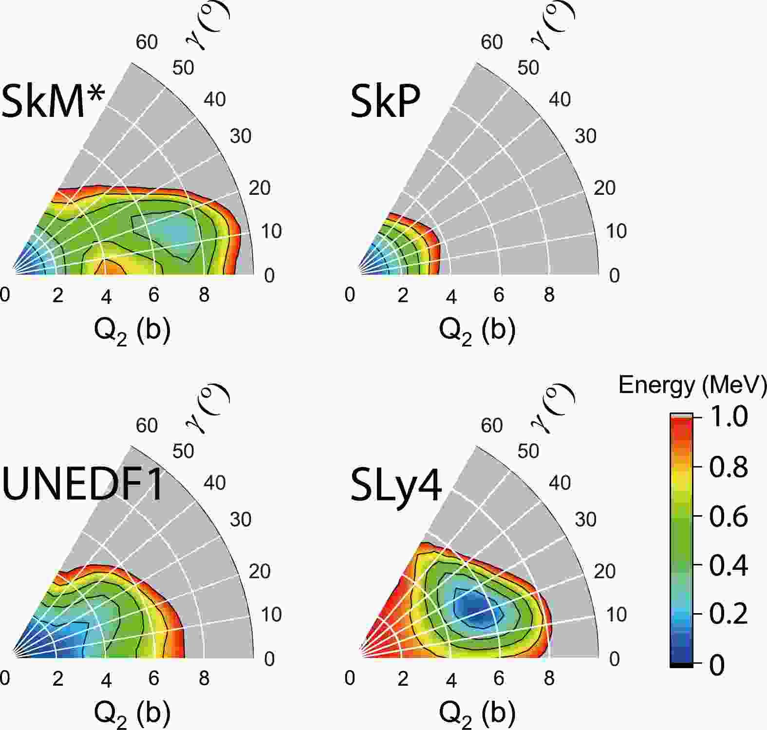
Figure 1 displays the calculated PESs using the four EDFs. All the EDFs predict spherical ground states, except for the SLy4 EDF, which predicts a triaxially deformed ground state. The SkM* EDF predicts an excited minimum at the triaxial deformation.

Figure 1

Figure 1.  (color online) Calculated potential energy surfaces using the SkM*, SkP, UNEDF1, and SLy4 EDFs. Neighboring contour lines are 200 keV apart in energy.

DownLoad: Full-Size Img PowerPoint

The lack of consistency among the parameterizations is because ¹⁰⁰Mo is predicted to be a transitional nucleus from spherical isotopes to the triaxially deformed ones [10]. In this transitional nucleus, the PES is softened by the pairing interaction. Previous random-phase approximation calculations based on axially-symmetric states with a small axial deformation have given a reasonable reproduction of the strength functions [18], whereas beyond-mean-field calculations using the Gogny force [19] seems to favor a well deformed triaxial ground state in ¹⁰⁰Mo [20]. The current study may shed new light on the evolution of ground-state deformations in Mo isotopes, particularly concerning triaxiality.

B ISM strength functions

• I. INTRODUCTION
• II. MODEL
• III. RESULTS AND DISCUSSIONS
•      A Ground state potential-energy surfaces
•      B ISM strength functions
•      C Coupling between isoscalar quadrupole andmonopole vibrations
• IV. SUMMARY
• ACKNOWLEDGMENTS

As displayed in Fig. 1, the PESs of ¹⁰⁰Mo exhibit a strong dependence on the EDFs used. In this section, we select a $\beta_2$ value near $(Q_{20},~ Q_{22})= (7.0,~ 0.0)$ b ($\beta_2\sim0.3$), which is close to the quadrupole moments of the minima calculated with the SkM* and SLy4 parameters. We also include a typical $\beta_2\sim0.16$, as selected in Ref. [18], to demonstrate the differences in the strength functions corresponding these $\beta_2$ values. After fixing these $\beta_2$ values, we perform TDDFT + BCS calculations by constraining the γ value at $0-30^{\circ}$, as suggested by the calculations using Gogny forces [19].

Figure 2 shows the ISM strengths calculated for a few deformations using the TDDFT + BCS method (SkM* EDF). For the smaller quadrupole deformations ($\beta_2= 0.16$), the main peaks at higher energy ($E\approx17$ MeV) are considerably more pronounced than the low-energy peaks. With increasing triaxial deformation γ, the lower-energy peaks for $\gamma=0^{\circ}$ at $E\approx13.5$ MeV become less distinguishable and become shoulders at $\gamma=30^{\circ}$.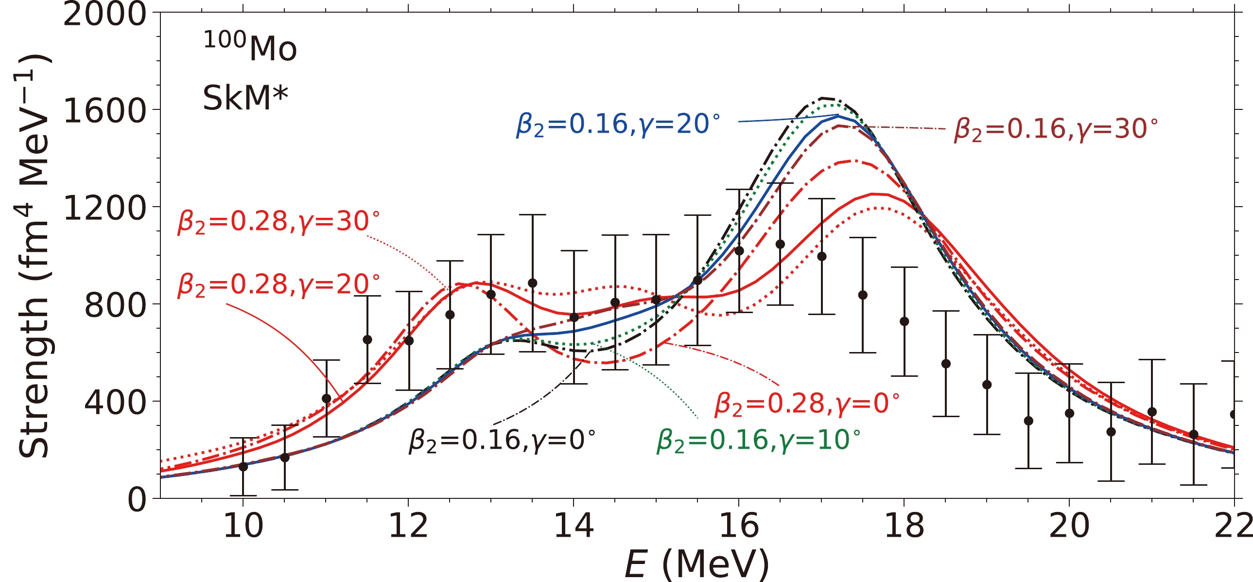

Figure 2

Figure 2.  (color online) ISM strengths calculated using the TDDFT method with the SkM* EDF. The experimental data are extracted from Refs. [6, 7].

DownLoad: Full-Size Img PowerPoint

For a larger $\beta_2=0.28$, the two peaks become more separate. With $\gamma=20^{\circ},30^{\circ}$, the low-energy peak separates into two peaks, forming a broader plateau joining the peak at higher energy. The main peaks occurring at higher energies $E\approx17.5$ MeV are considerably lower in height compared to those calculated based on a smaller $\beta_2=0.16$. For $\beta_2=0.28$, the height of the plateau in the low-energy region ($E\approx12-15$ MeV) is larger than that calculated with $\beta_2=0.16$.

In Fig. 2, the calculated strength functions are compared with the experimental data [6, 7]. It can be seen that all the calculations overestimate the energy of the second peak. The observed strength function peaks at $E\approx16.5$ MeV. The calculations overestimate the data by $\approx0.5$ and $\approx1.0$ MeV for $\beta_2=0.16$ and $\beta_2=0.28$, respectively. In Ref. [18], a number of EDFs with $K_{\infty}$ values ranging from 234 to 202 MeV have been used to calculate the single peaks of Mo isotopes. It is concluded that the ISM strengths in the Mo isotopes call for a smaller $K_{\infty}$ value. For the SkM* parameter, $K_{\infty}=217$ MeV. This value is larger than that of the SkP parameter ($K_{\infty}=202$ MeV), which contributes to the overestimation of the high-energy peak when compared with the data.

Nevertheless, for ($\beta_2,~\gamma$)=($0.28,~20^{\circ}/30^{\circ}$), the calculated strengths show features that reproduce the data both in the rising part and the general peak structure. Compared to the strength functions of a smaller $\beta_2$ value, those corresponding larger $\beta_2$ values are more spread and less pronounced. In particular, when the γ value is increased, the lower peak becomes a plateau, which is closer to the experimental data. In Sec. II.C, we attempt to explain the formation of the plateau in the lower-energy region. The flattening is due to the occurrence of an additional peak between the two existing peaks for the axially deformed nucleus. The additional peak is caused by the coupling of the ISM vibration mode with the isoscalar quadrupole vibration mode ($K=2$).

Figure 3 shows the strength functions calculated with the SkP EDF. This EDF has $K_{\infty}=202$ MeV, resulting in lower energy resonances compared with those of SkM*, as expected. The energy of the main peak, based on the results of $\beta_2=0.16$, is lower by 0.5 MeV compared to the data ($E\approx16.8$ MeV). Again, we notice that a larger $\beta_2$ value (0.25) together with triaxial deformation (30$^{\circ}$) can reproduce the general shape of the observed strength function.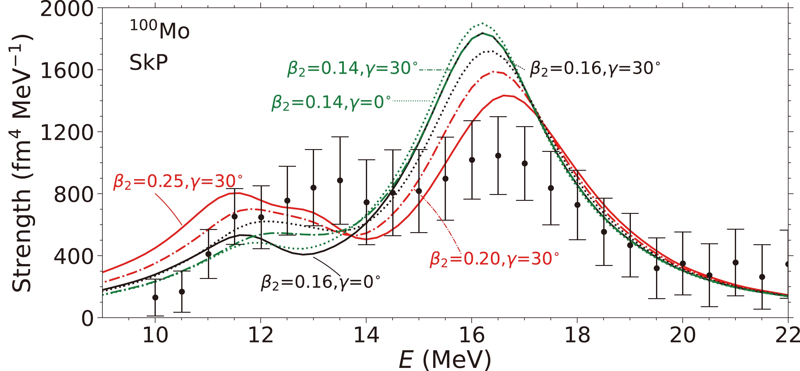

Figure 3

Figure 3.  (color online) Strengths corresponding to the response of the $Q_{20}$ ($S_{20}$), $Q_{21}$ ($S_{21}$), and $Q_{22}$ ($S_{22}$) moments.

DownLoad: Full-Size Img PowerPoint

Figure 4 displays the ISM strengths calculated using the UNEDF1 EDF. This parameterization is obtained by considering the properties of deformed nuclei. $K_{\infty}=220$ MeV for the UNEDF1 parameterization. Again, it is seen that the strengths at the lower-energy part can be reproduced by the calculation based on a deformation of $\beta_2\approx0.25,~0.30$. For the results of $\beta_2=0.25$, we include $\gamma=20^{\circ}$ and $30^{\circ}$, and it is clear that the increase in γ results in the plateaus between the two peaks. The heights of the calculated plateau part for $E\sim12-14$ MeV are lower than those of the other EDFs for UNEDF1. Consequently, this parameter requires a larger $\beta_2=0.3$ value to best reproduce the data.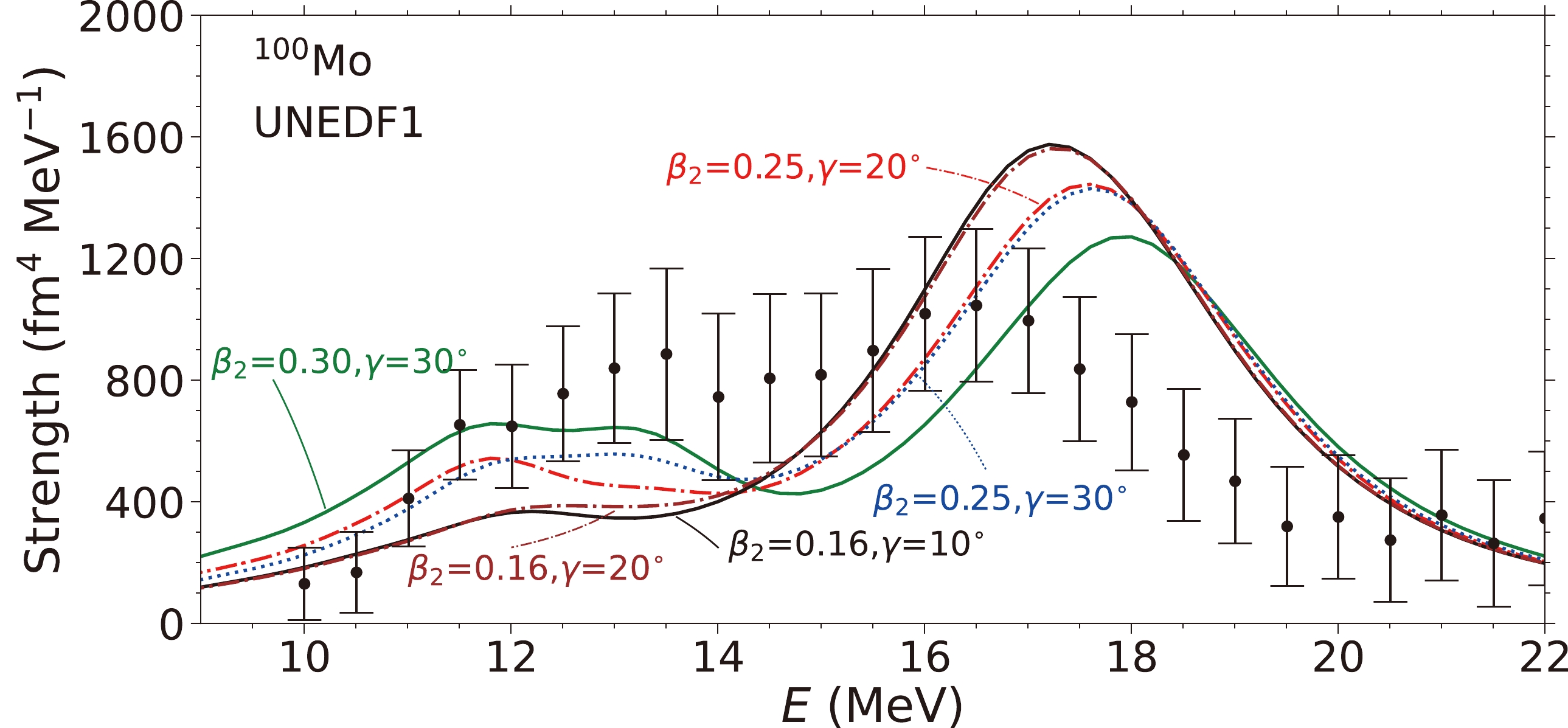

Figure 4

Figure 4.  (color online) Similar to Fig. 2, except for the SkP EDF.

DownLoad: Full-Size Img PowerPoint

Figure 5 displays the strengths calculated using the SLy4 EDF. For results based on a smaller deformation, $\beta_2\approx0.2$, similar curves are seen in the case of the SkM* EDF. For the strength based on a deformation of ($\beta_2$, γ)=(0.28, 30$^{\circ}$), we notice a similar agreement with the data as those given by the SkM* EDF at the same deformation (Fig. 2). However, the higher-energy peak is at $E\approx18.2$ MeV, which is $\sim$1.5 MeV higher than the observed one. This is due to the large $K_{\infty}=230$ MeV predicted by the SLy4 EDF.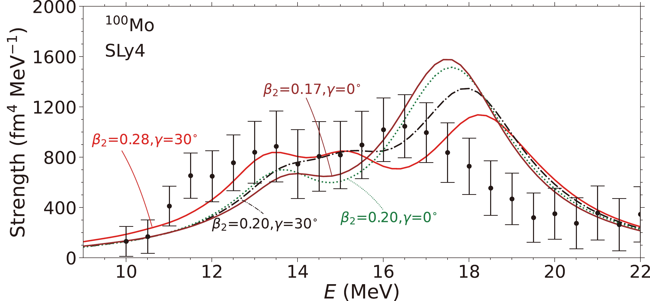

Figure 5

Figure 5.  (color online) Similar to Fig. 2, except for the UNEDF1 EDF.

DownLoad: Full-Size Img PowerPoint

One interesting observation is that all four EDFs predict similar widths for the strength functions at similar deformations. The SkM*, SLy4, and UNEDF1 EDFs reproduce the energy of the rising part of the observed strength function but overestimate the second peak, giving a broader general strength peak. The results with the SkP EDF underestimate the energy corresponding to the rising part but reproduce the second peak. We note that the FSUGarnet parameter of relativistic mean field theory seems to predict a narrower giant ISM peak in the spherical calculations [7].

C Coupling between isoscalar quadrupole andmonopole vibrations

• I. INTRODUCTION
• II. MODEL
• III. RESULTS AND DISCUSSIONS
•      A Ground state potential-energy surfaces
•      B ISM strength functions
•      C Coupling between isoscalar quadrupole andmonopole vibrations
• IV. SUMMARY
• ACKNOWLEDGMENTS

In Ref. [18], the low-energy shoulder was interpreted as a coupling between the isoscalar monopole and the isoscalar quadrupole vibration mode. A similar two-peak structure has been discussed for the ISM strengths of Sm isotopes in random-phase approximation calculations based on axial deformations [21–23]. These studies draw their conclusions from an examination of the isoscalar quadrupole strength functions that peak at a similar energy as that of the low-energy peak of the ISM strength function.

In this section, we numerically investigate the coupling using our TDDFT + BCS calculations [24]. We examine the strengths of the isoscalar quadrupole moments with $K=0,~1,~2$ after an ISM boost of the nucleus. By doing this, we gain information (such as the energy and relative coupling magnitude) about the modes that couple with the ISM vibration. It should be noted that in the TDDFT calculations, we do not enforce any symmetry on the wavefunctions and densities.

In Fig. 6 (upper panel), we plot the Fourier transform of the relevant quadrupole moments, $Q_{20,21,22}(t)$, after the ISM boost, which corresponds to the dotted red curves ($\beta,~\gamma)=(0.28,~30^{\circ}$) in Fig. 2. We note that the two quadrupole modes, $S_{20}$ and $S_{22}$, exhibit significant strengths at $E\approx12.5$ and 14.5 MeV, which are responsible for the first and second peaks in the low-energy region (see Fig. 2). The $S_{21}$ mode shows zero strength, suggesting no coupling between this mode and the ISM mode.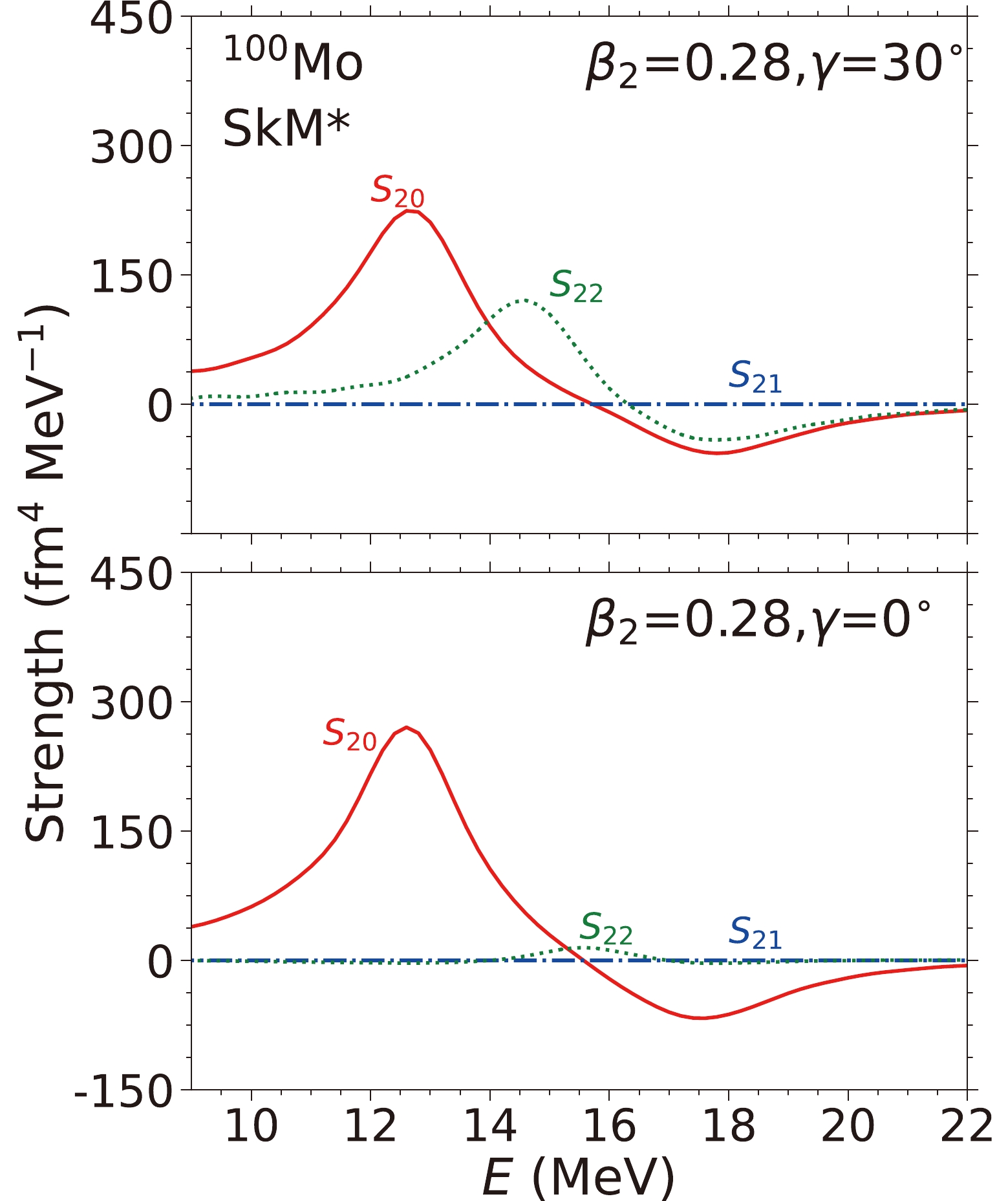

Figure 6

Figure 6.  (color online) Similar to Fig. 2, except for the SLy4 EDF.

DownLoad: Full-Size Img PowerPoint

Next, we qualitatively explain the behavior of $S_{20,21,22}$ in Fig. 6. For $\beta_2>0$ and $\gamma=0$ (lower panel of Fig. 6), we have

It follows that

meaning that the nuclear matter density extends further in the z direction than in the x and y directions. After an isotropic ISM boost, the magnitude of the extension/contraction of the nucleus in the z direction is expected to be different from those in the x and y directions. This results in the $Q_{20}$ varying with time. The $Q_{22}$ value remains zero because this boost is isotropic. The magnitudes of breathing in the x and y directions are the same.

For $\beta_2>0$ and $\gamma\neq 0$ (upper panel of Fig. 6), the $K=0$ mode of the isoscalar quadrupole vibration still couples with the ISM vibration as explained in the previous paragraph. Now, $Q_{22}\neq0$ and $\langle x^2 \rangle \neq \langle y^2 \rangle$ in the static calculation. After the boost, the matter distribution in the x and y directions varies differently around the static values. Hence, $S_{22}$ becomes nonzero.

In the above two scenarios, similar reasonings can be applied to the $S_{21}$ ($Q_{21}\equiv\langle xz \rangle$) case too. In this case, an ISM boost will not make the density lose the $xy$-, $xz$-, or $yz$-plane flip symmetry (simplex symmetries) that the nucleus possesses in the beginning. The moments with an odd number of coordinates (such as $\langle x,y,z \rangle$, $\langle xy,yz, xz \rangle$,...) remain zero. Consequently, $Q_{21}$ remains zero during the course of the breathing of the nucleus.

The strengths for $Q_{22}$ and $Q_{2-2}$ are the same if they are defined as time-reversal partners, such as

In such a case, the ground state of the e-e nucleus preserves the time-reversal symmetry and $\langle Q_{22} \rangle = \langle Q_{2-2} \rangle$ always. However, in our case, $Q_{22} \sim x^2-y^2$, and $Q_{2-2} \sim xy$. For a triaxial ground state, $\langle Q_{22} \rangle$ has a finite value, whereas $\langle Q_{2-2} \rangle \sim \langle xy \rangle$ vanishes when the triaxial nucleus is placed inside a principle axis system. See Eqs. (8) and (9) of Ref. [25] for the reason behind the vanishing moments mentioned above.

In other words, axial quadrupole deformation allows the ISM resonance to couple with the $S_{20}$ ($K=0$) quadrupole mode, whereas triaxial deformation allows further coupling to the $S_{22}$ ($K=2$) mode. The $K=1$ quadrupole vibration would not couple with the ISM vibration. Decoupling the $K=1$ vibration mode from the spurious collective rotations is known to be difficult. In our time dependent simulation, the coupling between the ISM vibration and the spurious rotations is not observed (see Fig. 6 for the absence of the rotation within the $xz$ plane).

IV. SUMMARY

• I. INTRODUCTION
• II. MODEL
• III. RESULTS AND DISCUSSIONS
•      A Ground state potential-energy surfaces
•      B ISM strength functions
•      C Coupling between isoscalar quadrupole andmonopole vibrations
• IV. SUMMARY
• ACKNOWLEDGMENTS

In summary, we study the strength function of the isoscalar monopole (ISM) mode in ¹⁰⁰Mo using symmetry-unrestricted 3D TDDFT including a BCS pairing.

As the first step, we perform constrained HF + BCS calculations to obtain PESs using the SkM*, SkP, UNEDF1, and SLy4 EDFs. The first three EDFs predict spherical ground states, with SkM* and UNEDF1 showing softness in the triaxial deformation. The results with the SLy4 EDF show a triaxial minimum.

Except for those with SkP, the ground states with different EDFs seem to show triaxial softness. We constrain the ground state to a few sampling deformations before the time-dependent study.

The calculated strength functions using TDDFT + BCS exhibit two peaks if the axial deformation $\beta_2$ is in the region of $0.25-0.30$ and $\gamma=0^{\circ}$. Increasing the triaxial parameter γ results in the occurrence of a peak between the two existing peaks and the formation of a plateau area in the low-energy region ($E\sim12-14$ MeV). When $(\beta_2,~\gamma)= (0.28,~30^{\circ})$, the calculated strengths reproduce the experimental data. Hence, our microscopic calculations suggest a medium $\beta_2=0.25-0.3$ and static triaxial deformation ($\gamma=0-30^{\circ}$) in the ground state of ¹⁰⁰Mo.

Our time-dependent study allows us to investigate the time response of quadrupole moments after an ISM boost. The analyses show that the occurrence of the low-energy peaks is due to a coupling of the ISM mode and two isoscalar quadrupole modes ($K=0,2$).

ACKNOWLEDGMENTS

• I. INTRODUCTION
• II. MODEL
• III. RESULTS AND DISCUSSIONS
•      A Ground state potential-energy surfaces
•      B ISM strength functions
•      C Coupling between isoscalar quadrupole andmonopole vibrations
• IV. SUMMARY
• ACKNOWLEDGMENTS

YS thanks the HPC Studio at the Physics Department of the Harbin Institute of Technology for computing resources allocated through INSPUR-HPC@PHY.HIT.

References