Analysis of ${{\boldsymbol b}{\bf\rightarrow} {\boldsymbol c}{\boldsymbol\tau}\bar{\boldsymbol\nu}_{\boldsymbol\tau}}$ anomalies using weak effective Hamiltonian with complex couplings and their impact on various physical observables

High-energy physics accelerators are used to directly search for new particles, which can be intermediate quantum states, also known as resonances. These quantum states often decay quickly and can be observed by detecting their decay products. The heavy to light semileptonic decays of b−hadrons are important for indirectly hunting for the new physics (NP). Among them, the decays induced by the Flavor Changing Neutral Current (FCNC) transitions, i.e., $ b\to (d,s) $, are crucial to testing the Standard Model (SM) precisely and searching for possible deviations from it. Particularly, the rare semi-leptonic B meson decays are useful for investigating the Higgs Yukawa interaction by testing Lepton Flavor Universality (LFU), which is a ratio with different generations of leptons in the final state. LFU is approximately 1 in the SM, with a small breaking owing to lepton masses in the decay phase space. The measured values of the branching ratios and angular distributions of FCNC decays, $ B^{\pm }\to K^{(*)\pm }\ell^{+}\ell^{-} $, $ B^{0}\to K^{0}\ell^{+}\ell^{-} $, and $ B_{s}^{0}\to\phi\ell^{+}\ell^{-} $, where $ \ell=\mu,\;e $, exhibited some deviations from SM predictions [1–7]. Several studies have been conducted to accommodate these deviations, see, e.g., [8–13] and the references therein.

In contrast to the CKM-suppressed FCNC decays, which occur at a loop level in the SM, decays involving the quark level Flavor Changing Charged Current (FCCC) transitions $ b\rightarrow c\ell\nu_{\ell} $ ($ \ell=e,\mu,\tau $) have no such suppression. Interestingly, similar tensions with the SM predictions have been observed in FCCC exclusive decays, $ B\rightarrow D^{(*)}\ell\nu_\ell $, $ B\rightarrow J/\psi\ell\nu_\ell $, $ \Lambda_{b}\rightarrow \Lambda_{c}\ell\nu_\ell $, providing an opportunity to mark several physical observables to test the results of the SM. Theoretically, these exclusive decays are prone to uncertainties resulting from the form factors (FFs) (non-perturbative inputs) and errors in the CKM matrix elements. However, the dependence on the CKM elements and uncertainties from FFs are mitigated if we obtain the ratio of the branching fractions $ ({\cal{B}}) $ in these semi-leptonic decays, i.e.,

In the SM, the heavy-quark effective theory and lattice QCD approach have been used to study the LFU ratio $ R_{\tau/\mu,e}\left(D^{(*)}\right) $[14–24]. The corresponding SM results are

These theoretical results were scrutinized using measurements from BABAR, Belle, and LHCb, where the experimental measurements of $ R_{\tau/{\mu, e}}\left(D^{(*)}\right) $ by BABAR [25, 26], Belle [27–29], and LHCb [30–34] had significant deviations from the SM predictions. Recently, the Heavy Flavor Averaging Group (HFLAV) updated their earlier results of $ R_{\tau/{\mu, e}}\left(D\right) $ and $ R_{\tau/{\mu, e}}\left(D^{*}\right) $ [35, 36], and the current world averages [37] exceed the SM predictions by $ 2.0\sigma $ and $ 2.2\sigma $, respectively. Invoking the correlation of –0.37 between these universality ratios, the HFLAV global averages are

deviating from the SM predictions by $ 3.3\sigma $ [37]. However, the SM determination is improved by calculating the next-to-leading order QCD corrections for $ B\to D^{(*)} $ form factors [38].

Owing to the spins of the final state particles $ D^* $ and the lepton in $ B\to D^* \ell \bar{\nu}_\ell $, the associated polarization asymmetries are useful for checking the consistency of the NP observed in various LFUs. Experimentally, the lepton polarization asymmetry $ P_\tau\left(D^{*}\right) $ and the longitudinal polarization fraction of $ D^{*} $ meson, i.e., $ F_{L}(D^{*}) $ were measured by Belle [39, 40, 41]:

which lie within $ 1.5\sigma $ of the SM prediction [42, 43]:

The incompatibility of these measurements with SM predictions is a key aspect in discriminating different NP models.

In the charmed B−meson decay $ B_c\to J/\psi \ell \nu_\ell $, occurring through the same $ b\to c $ quark level transition, the LFU ratio $ R_{\tau/\mu}\left(J/\psi\right) $ was analyzed by the LHCb collaboration [44] at $ 7 $ and $ 8 $ TeV center of mass energies of proton-proton collisions with an integrated luminosity of $ 3fb^{-1} $. The mismatch between the experimentally measured value [44]

and the SM prediction [45, 46]

is $ 1.8\sigma $. Similar to these LFU ratios, we can define the ratio for the inclusive B-meson decay $ B\to X_c\tau\bar{\nu}_{\tau} $

where the SM result $ 0.216\pm 0.003 $ [47] lies within $ (\; 0.2\sigma) $ of the experimental measurements [48]:

We know that the LHCb is quite rich in producing b−hadrons and the ratio of $ B : \Lambda_b $ is 2:1, providing an opportunity to study the Cabibbo suppressed decay modes of $ \Lambda^0_b $ [49–53]. Analogous to the ratios of B meson decays, the ratio $ R_{\tau/\ell}(\Lambda_{c}) $ involving the $ \Lambda_{b} $ baryon decay, has also been measured by the LHCb collaboration for $ \Lambda_{b}\rightarrow \Lambda_{c}\tau\nu_\tau $ decays [54]:

where the first, second, and third uncertainties are due to the statistical, system, and external branching fractions measurements, respectively. This experimental value conflicts with the corresponding SM result [55, 56] ($ 0.324\pm 0.004 $) by $ 1.8\sigma $. The underabundance of taus in these $ \Lambda_b $ decays compared with the other ratios involving $ b \to c \tau \bar{\nu}_\tau $ is a perplexing behavior.

Considering left-handed (LH) neutrinos, these incompatibilities between the SM predictions and experimental measurements were explored through the NP dimension six operators in $ b\rightarrow c\tau\overline{\nu}_{\tau} $ transitions [57–69]. Including right-handed (RH) neutrinos and/or the RH quark currents in the model independent WEH, several studies analyzed these anomalies, see e.g., [70–80]. Particularly with the assumption of LH neutrinos, using the experimental measurements of $R_{\tau /{\mu,e}}\left(D\right), R_{\tau/{\mu,e}}\left(D^*\right), \sim R_{\tau/{\mu,e}}\left(J/\psi\right)$, and $ F_{L}\left(D^*\right) $, Blanke et al. [65] elegantly analyzed four one-dimensional scenarios with real Wilson coefficients (WCs), $ C^{V}_L, C^{S}_R, C^{S}_L $, and $ C^{S}_{L}=4C^T $, where the subscripts indicate the Lorentz structure of the current corresponding to these WCs in the WEH. Focusing on the same experimental observables, they further extended their analysis to 2D scenarios by considering only $ C^{S}_L=4C^{T} $ to be the complex-valued. The scenarios deeply influence the branching ratio of $ B_{c}\rightarrow \tau\nu_\tau $ decay, which has not been measured yet owing to a large uncertainty in the lifetime of $ B_c $ meson [81, 82] is not measured yet; therefore, upper limits of 60%, 30%, and 10% on the contribution from $ B_{c}\rightarrow \tau\nu_\tau $ to total $ B_{c} $ decay width have been imposed in literature [83–88]. This impacts the parametric space for these NP WCs, and Ref. [65] reported that, for the 10% limit, the only scenario $ C^R_S $ departs the fit from measurements; whereas, in 2D scenarios, the fit is valid for two out of four benchmark scenarios. Later, with these constraints on the available parametric space of the NP WCs, the values of $ P_T\left(D^*\right) $ and $ R_{\tau/\ell}(\Lambda_{c}) $ were predicted for both cases.

Now, after this detailed overview of the theoretical and experimental studies, the work presented here has two important features. In the first step, using the model-independent WEH with LH neutrinos and complex NP Wilson coefficients, we use the most up-to-date HFLAV world average summer 2023 [37] values for $ R_{\tau/\mu,e}(D) $ and $ R_{\tau/{\mu,e}}(D^{*}) $ and the measurements of $F_{L}\left(D^{*}\right),\; P_{\tau}\left(D^{*}\right), R\left(J/\psi\right)$, and $ R_{\tau/\ell}\left(X_c\right) $ given in Eqs. (1)−(10) to revisit the global fit analysis. Although we have complex NP WCs, we employ the same technique developed in [65] to scrutinize NP parametric space for real WCs. In this scenario, we analyze $ \chi^{2} $ by considering two sets of physical observables. In set $ {\cal{S}}_1 $, we select $ R_{\tau/\mu,e}(D), R_{\tau/{\mu,e}}(D^{*}), F_{L}\left(D^{*}\right) $, and $ P_{\tau}\left(D^{*}\right) $, whereas in $ {\cal{S}}_2 $, we include $R_{\tau/\mu}\left(J/\psi\right)$ and $ R_{\tau/\ell}(X_{c}) $ in the list. The objective of these two sets is to scrutinize the parametric space of the new WCs. For the set $ {\cal{S}}_1 $, we find that the effect of the NP scalar WC $ C^{L}_S $ is prominent compared with the other WCs, and it also exhibits a strong dependence on the constraints resulting from the branching ratio of $ B_c \to \tau \nu $. Expecting the p-values to be ~50% for a true solution, we observe a less favorable alignment with the observed anomalies for the set $ {\cal{S}}_2 $.

Correlation studies of the various observables associated with these decay modes will be important tools for the indirect detection of NP, the LFU ratios $ R_{\tau/{\mu,e}}\left(D\right) $, $ R_{\tau/{\mu,e}}\left(D^*\right) $, and $ R_{\tau/{\ell}}\left(\Lambda_{c}\right) $ are correlated in a model-independent manner [65, 66]. The relation of $ R_{\tau/{\ell}}\left(\Lambda_{c}\right) $ with the well measured $ R_{\tau/{\mu,e}}\left(D\right) $, $ R_{\tau/{\mu,e}}\left(D^*\right) $ is known as the sum-rule, and it was derived in [65] and further updated in [66].

In the second step, we find similar relations/sum-rules for the other LFU ratios $R_{\tau/{\mu,e}}\left(J/\psi\right)$ and $ R_{\tau/\ell}(X_{c}) $ by expressing them in terms of $ R_{\tau/\mu,e}(D) $ and $ R_{\tau/{\mu,e}}(D^{*}) $ and calculate their numerical values including the uncertainties from the SM inputs and experimental measurements of $ R_{\tau/\mu,e}(D) $ and $ R_{\tau/{\mu,e}}(D^{*}) $. In addition to this correlation established through these sum rules, we determine their correlation with $ R_{D} $ and $ R_{D^*} $ by plotting them for particular values of NP WCs in $ {\cal{S}}_1 $. Finally, we study the impact of these NP WCs on the physical observables such as the CP even and odd angular observables in $B\to D^*\left(\to D\pi\right) \tau \bar{\nu}_\tau$ decays and the different CP asymmetry triple products.

The remainder of this paper is organized as follows. In Sec. II, after defining the WEH containing the SM and NP operators, we present the formulas of the observables $ R_{\tau/{\mu,e}}\left(D\right) $, $ R_{\tau/{\mu,e}}\left(D^{*}\right) $, $ P_{\tau}(D^{*}) $, $ F_{L}(D^{*}) $, $ R_{\tau/\mu}(J/\psi) $, $ R_{\tau/\ell}(X_{c}) $, and $ R_{\tau/\ell}\left(\Lambda_{c}\right) $ in terms of the NP WCs. Considering the most recent data, in Sec. III, we analyze the parametric space of our complex NP WCs and discuss the impacts of the limits on the branching ratio of $ B_c\to \tau \bar{\nu}_\tau $ on the allowed regions of these WCs. In Sec. IV, we derive the sum rules for $R_{\tau/{\mu}}\left(J/\psi\right)$ and $ R_{\tau/\ell}(X_{c}) $ in terms of $ R_{\tau/\mu,e}(D) $ and $ R_{\tau/{\mu,e}}(D^{*}) $ and discuss the correlation amongst the physical observables. Sec. V discusses the impact of these constraints on polarized branching ratios and various $ CP $ even and odd angular observables and the $ CP $ asymmetry triple products in $ B\to D^*\tau\bar{\nu}_\tau $ decays. Finally, in Sec. VI, we conclude our findings. This work is supplemented by three appendices discussing the fitting procedure and derivation of the above-mentioned $ CP $ asymmetries.

In the absence of experimental evidence for deviations from the SM predictions at tree-level transitions involving light leptons, NP is generally believed to play a role in the third-generation fermions, i.e., τ. Regarding this, to explore any possible NP in the $ b\to c\tau\bar{\nu}_\tau $ transition, we consider the WEH containing new dimension-six vector, scalar, and tensor operators with complex WCs. After integrating out the heavy degrees of freedom, we can express the WEH for $ b\to c\tau\bar{\nu}_\tau $ transition as [59, 65, 89–93]

Here, $ G_{F} $ is the Fermi coupling constant, and $ V_{cb} $ is the CKM matrix element. The first term is the SM contribution, and its corresponding WC is normalized to unity, i.e., $ \left(C_{L}^{V}\right)_{SM}=1 $. Ignoring the small mass of neutrinos and the RH vector currents for quarks, the operators $ O_V^L $, $ O_S^R $, $ O_S^L $, and $ O_T $ are given by [94–96]

where $ P_{R,L}=\left(1\pm \gamma_{5}\right)/2 $ are the projection operators, where the plus (minus) sign represents the right(left)-handed chiralities. The corresponding NP WCs are $ C_{R,L}^{X} $, where the upper index X represents scalar, vector, and tensor contributions, whereas the lower indices $ R,L $ denote quark-current chiral projections. As we have only considered the LH neutrinos, the lepton chirality index is not specified in the subscript of the NP WCs.

The values of the NP WCs depend on the renormalization scale of the theory. Note that $ b\to c\tau\bar{\nu}_\tau $ transitions occur at the $ m_b $ scale, whereas the NP WCs are determined at a scale of heavy NP particles, which may set at 1 TeV [65] or 2 TeV [66]. The WCs at $ m_b $ and 1 TeV scales are connected by the Renormalizable Group equations (RGEs), and the corresponding relationships are [65, 97]

For the WEH given in Eq. (11), the expressions of the physical observables under consideration can be expressed in terms of the NP WCs at a scale $ \mu_b = m_{b} $ as [45, 47, 59, 66, 75, 89, 91, 98, 99]

Similarly, the branching ratio of the $ B_c \to \tau \bar{\nu}_\tau $ decay is expressed as

where in the SM, $ {\cal{B}}\left(B_{c}^{-}\rightarrow \tau^{-}\bar{\nu}_{\tau}\right)^{{\rm{SM}}}\approx 0.022 $ [99].

In this section, we scrutinize the parametric space for the NP complex WCs. We follow the same $ \chi^2 $ fitting technique that is developed for real WCs in [65], and it is summarized in Appendix A. In addition to the complex WCs in our case, the other differences from [65] are as follows: we have incorporated the most updated results of observables from HFLAV [37], and in Eqs. (14)−(20), the latest values of the FFs are used. Furthermore, based on the number of experimentally measured observables included in the analysis, we consider two different sets, namely

● In Set 1 $ ({\cal{S}}_1) $, by selecting $ R_{\tau/\mu,e}(D), R_{\tau/{\mu,e}} (D^{*}), F_{L}\left(D^{*}\right) $, and $ P_{\tau}\left(D^{*}\right) $, we determine the best-fit points (BFP) for these complex WCs, along with $ 1\sigma $ and $ 2\sigma $ variations.

● In Set 2 $ ({\cal{S}}_2) $, we add the two more observables $ R_{\tau/\mu}(J/\psi) $ and $ R_{\tau/\ell}\left(X_c\right) $ to $ {\cal{S}}_1 $ and observe if we could further constrain the parametric space of these NP WCs.

Owing to the complexity of NP WCs, to perform the $ \chi^2 $ analysis, the number of parameters, $N_{\rm par}$, is equal to 2, and $N_{\rm obs}$ is equal to 4 and 6 for $ {\cal{S}}_1 $ and $ {\cal{S}}_2 $, respectively. Thus, the numbers of degrees of freedom (dof) $N_{\rm dof}=N_{\rm obs}-N_{\rm par}$ are 2 and 4 for $ {\cal{S}}_1 $ and $ {\cal{S}}_2 $, respectively. The p-value quantifies the goodness of fit, and it is attributed to the probability of difference between the theoretical (SM) and experimental values. This can be hypothesized as

where $f(z;N_{\rm dof})$ is the $ \chi^{2} $ probability distribution function. As $N_{\rm par}=0$ for the SM, the p-value is very small $ \left(\approx 10^{-3}\right) $ [65]. Our main objective is to estimate the BFP, p−value, $ \chi_{{\rm{SM}}}^{2} $, $ {\rm{pull}}_{{\rm{SM}}} $, and $ 1\sigma $, $ 2\sigma $ intervals for the WCs.

Note that the parametric space of the WCs depends on the constraints on the branching ratio of a helicity suppressed SM decay mode $ B^-_{c}\to \tau^- \bar{\nu}_\tau $, which has not been precisely measured yet (see e.g., [65] for an elaborate discussion). However, we have some experimental bounds on it; therefore, to impose the cuts on the allowed parametric space, we must place some upper bounds on the branching ratio of this decay. First, we consider the most conservative bound of <60% contribution of the $ B^-_{c}\to \tau^- \bar{\nu}_\tau $ decay rate to the total decay width of $ B_c $ meson, then take the commonly used <30% and finally a hypothetical future limit of <10% [65].

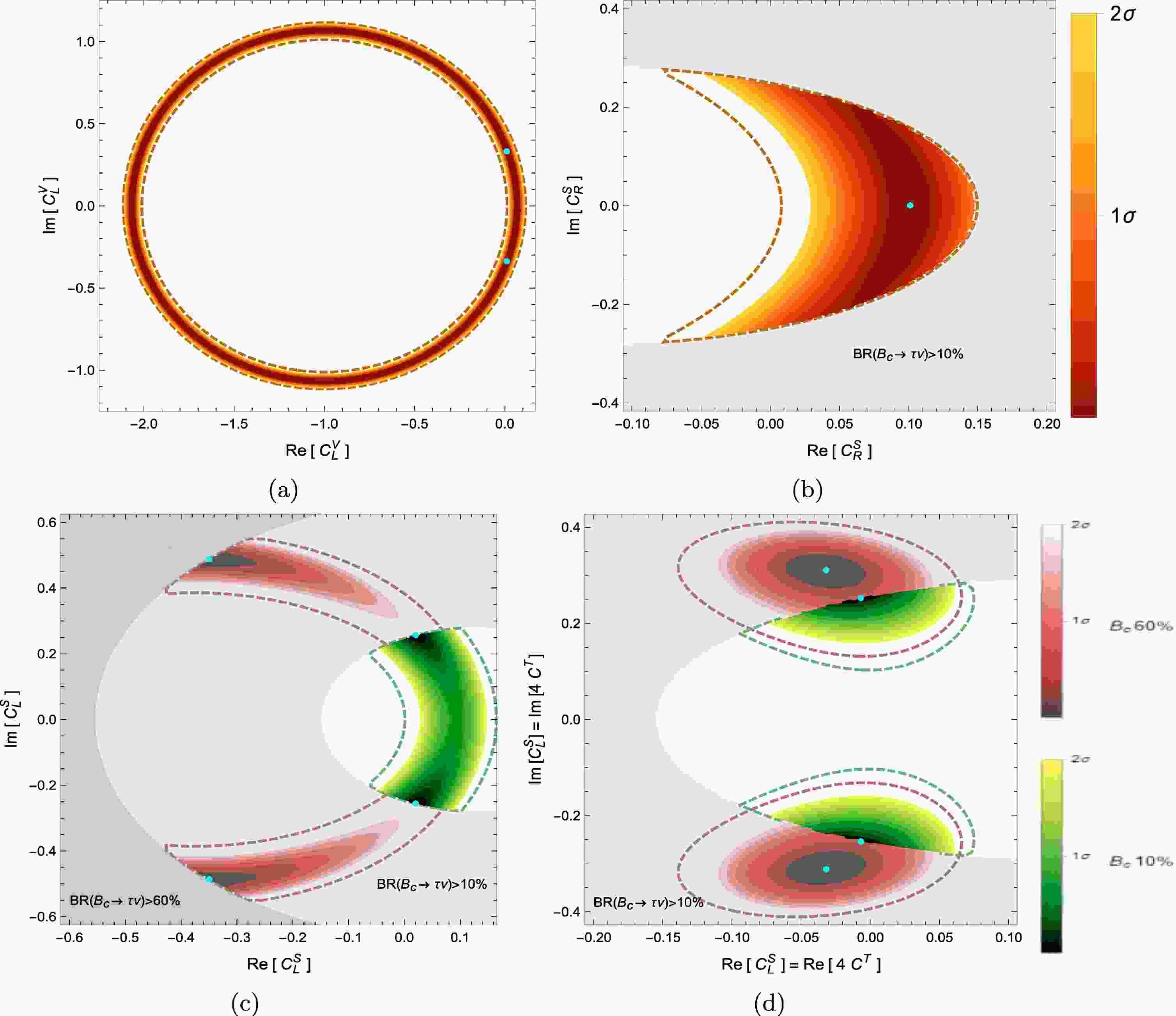
In our analysis, we adopt the strategy of switching on one NP WC at a time, and the corresponding results are shown in Fig. 1 for both sets of $ {\cal{S}}_{1} $ (solid colors) and $ {\cal{S}}_2 $ (dotted lines). We have also included the 10% and 60% constraints of $ {\cal{B}}\left(B^-_c\to \tau^- \bar{\nu}_\tau\right) $, indicated by light and dark gray colors, respectively. Any point lying inside the gray shades depicts the disallowed parametric space corresponding to a particular limit on the branching ratio. The description of various colors is given in the caption of Fig. 1.

Figure 1.  (color online) Results of the fits for NP scenarios. The light and dark gray colors show the 10% and 60% branching ratio constraints, respectively. The light (dark) color contours represent the $ 1(2\sigma) $ deviations from the BFP (cyan color). Panels (a), (b), (c), and (d) show the ranges of real and imaginary parts of $ C_{L}^{V} $, $ C_{R}^{S} $, $ C_{L}^{S} $, and $ C_{L}^{S}=4C^{T} $, respectively, restricted by $ {\cal{S}}_1 $. The contours indicated by dotted lines show the maximum limit of the $ 2\sigma $ region for set $ {\cal{S}}_2 $. In Fig. 1 (a) and (b), the (orange color coding) is not affected by either of these constraints, whereas in Fig. 1 (c) and Fig. 1 (d), the red and green colors coding are the 60% and 10% constraints, respectively. The cyan dots show the BPF in the two sets.

● Fig. 1 (a) plots the allowed parametric space of $ C^{V}_L $. We can observe that for $ C^{V}_L $, the parametric space is independent of the constraints from $ {\cal{B}}\left(B^-_c\to \tau^- \bar{\nu}_\tau\right) $, which is not the case for the real WCs [65]. The corresponding real and imaginary values of the BFP, $ \chi^2_{{\rm{min}}} $, the percentage $ p\text{-}{\rm{value}} $, $ {\rm{pull}}_{{\rm{SM}}} $, and $ 1\sigma $, $ 2\sigma $ ranges around BFP are given in Table 1. We can observe that, going from the $ {\cal{S}}_1 $ (solid colors) to $ {\cal{S}}_2 $ (dotted lines), the corresponding BFP value is reduced by 38%. Additionally, the $ p $-value is reduced by 30%, making it less likely to fit the anomalies. Additionally, the $ 1\sigma $ and $ 2\sigma $ ranges around the BFP are indicated by light and dark colors for $ {\cal{S}}_1 $ and $ {\cal{S}}_2 $, respectively. Here, the dotted line represents the maximum of $ 2\sigma $ for $ {\cal{S}}_2 $.

Set $ {\cal{S}}_1\left({\cal{S}}_2\right) $ ($ \chi_{{\rm{SM}}}^{2}=17.22\left(20.53\right) $, $p\text{-}{\rm{value} }=1.75\left(3.38\right)\times10^{-3}$)
WC	BR	BFP	$ \chi_{{\rm{min}}}^{2} $	$p\text{-}{\rm{value} }$ %	$ {\rm{pull}}_{{\rm{SM}}} $	$ 1\sigma $-range	$ 2\sigma $-range
$ C_{L}^{V} $	–	$ (0.01,\pm 0.33) $	2.76	25.2	3.8	$ [-2.09,0.09],[-1.09,1.09] $	$ [-2.11,0.11],[-1.11,1.11] $
		$ (-0.03,\pm 0.45) $	6.31	17.7	3.77	$ [-2.1,0.1],[-1.1,1.1] $	$ [-2.12,0.12],[-1.12,1.12] $
		38%	3.56	–30%	–0.03	1%	1%
$ C_{R}^{S} $	–	$ (0.1,0) $	5.67	5.9	3.4	$ [0,0.14],[-0.25,0.25] $	$ [-0.05,0.03],[-0.27,0.27] $
		$ (0.1,0) $	9.18	5.7	3.37	$ [-0.04,0.04],[-0.27,0.27] $	$ [-0.08,0.01],[-0.28,0.28] $
		0%	3.51	–3%	–0.03	14%	4%
$ C_{L}^{S} $	<60%	$ (-0.35,\pm 0.49) $	0.89	64.1	4.04	$ [-0.39,-0.15],[-0.53,0.53] $	$ [-0.42,0.02],[-0.55,0.55] $
		$ (-0.42,\pm 0.48) $	4.36	35.9	4.02	$ [-0.41,-0.03],[-0.54,0.54] $	$ [-0.44,0.12],[-0.55,0.55] $
		12%	3.47	–44%	–0.02	13%	10%
	<30%	$ (-0.13,\pm 0.41) $	3.65	16.1	3.68	$ [-0.17,-0.02],[-0.43,0.43] $	$ [-0.2,0.11],[-0.45,0.45] $
		$ (-0.13,\pm 0.41) $	7.07	13.2	3.67	$ [-0.19,0.06],[-0.44,0.44] $	$ [-0.21,0.15],[-0.45,0.45] $
		0%	3.42	–18%	–0.01	12%	5%
	<10%	$ (0.02,\pm 0.26) $	7.26	2.7	3.16	$ [-0.02,0.1],[-0.27,0.27] $	$ [-0.05,0.15],[-0.28,0.28] $
		$ (0.02,\pm 0.26) $	10.65	3.1	3.14	$ [-0.04,0.13],[-0.27,0.27] $	$ [-0.07,0.16],[-0.28,0.28] $
		0%	3.38	17%	–0.02	9%	5%
$ C_{L}^{S}=4C^{T} $	$ \begin{array}{c} <60\% \\ \& \\ 30\% \end{array} $	$ (-0.03,\pm 0.31) $	2.69	26.1	3.81	$ [-0.08,0.02],[-0.37,0.37] $	$ [-0.11,0.05],[-0.4,0.4] $
		$ (-0.04,\pm 0.31) $	5.98	20.1	3.81	$ [-0.11,0.04],[-0.38,0.38] $	$ [-0.14,0.07],[-0.41,0.41] $
		3%	3.29	–23%	0.	7%	7%
	<10%	$ (-0.01,\pm 0.25) $	4.51	10.5	3.56	$ [-0.05,0.03],[-0.27,0.27] $	$ [-0.07,0.06],[-0.28,0.28] $
		$ (-0.01,\pm 0.25) $	7.74	10.2	3.58	$ [-0.07,0.05],[-0.28,0.28] $	$ [-0.09,0.07],[-0.28,0.28] $
		0%	3.23	–3%	0.02	8%	7%

Table 1.  Results of the fit for complex WCs including BFP $ ({\rm{Real}},\; {\rm{Imaginary}}) $, $ \chi_{{\rm{min}}}^{2} $, $p\text{-}{\rm{value}}$ %, $ {\rm{pull}}_{{\rm{SM}}} $, $ 1\sigma $, and $ 2\sigma $-ranges of $ ({\rm{Real}},\;{\rm{Imaginary}}) $ parts of the corresponding WCs. The numbers are given after placing the bounds on $ {\cal{B}}\left(B^-_{c}\to\tau^-\bar{\nu}_\tau\right)<60\%, 30\% $, and <10% for both sets of observables i.e., $ {\cal{S}}_1 $ and $ {\cal{S}}_2 $. In each sub-row of WCs, the first, second, and third rows represent data for sets $ {\cal{S}}_1, {\cal{S}}_2 $, and the difference between the values obtained from the two sets, respectively.

● Figure 1 (b) represents the allowed regions for $ C^{S}_R $ for sets $ {\cal{S}}_1 $ and $ {\cal{S}}_2 $ with the color description being the same as in Fig. 1 (a). The $ 1\sigma $ and $ 2\sigma $ ranges lie beyond the 10% constraints of the branching ratio. Table 1 shows that for the BFP the imaginary component of $ C^{S}_R $ is zero to a given accuracy, and the corresponding $ p $-value is small. However, for the corresponding $ 1\sigma $ and $ 2\sigma $ intervals, this is not the case, as the real and imaginary components are of equal weight here.

● Compared with $ C^{V}_L $ and $ C^{S}_R $, the complex WC $ C_{L}^{S} $ is notably influenced by the branching ratio constraints for both sets $ {\cal{S}}_1 $ and $ {\cal{S}}_2 $. This dependence is expected because the SM helicity suppression of $ B_c\to \tau^{-}\bar{\nu}_\tau $ is lifted owing to these left-handed scalar/pseudo-scalar type operators. For $ {\cal{S}}_1 $, for a 60% bound on the branching ratio, its $ p $-value is 64%. However, for the commonly used bound of 30% on it, the $ p $-value decreases by quarter 16%, and in the hypothetical future limit 10%, this value reduces to only 2.7%, disfavoring the pseudo-scalar explanation of the data. In contrast to $ {\cal{S}}_1 $, in set $ {\cal{S}}_2 $, the $ p $-value is already reduced by a factor of half even for the 60% bound on the branching ratio. This is caused by the large uncertainty in the measurement of $ R_{\tau/\mu}\left(J/\psi\right) $. In Fig. 1 (c), we have plotted the corresponding BFP and the $ 1\sigma $ and $ 2\sigma $ ranges. We observe that the large parametric space is available when we consider the 60% limit, and this reduces when we apply the 10% bound, justifying our findings presented in Table 1.

● Furthermore, our fourth scenario, which is $ C_{L}^{S}=4C^{T} $, exhibits moderate sensitivity only when the stringent future limit of <10% on the branching ratio is used. It reduces the $ p $-value from 26% to 10% when we change $ {\cal{B}}\left(B^-_c\to \tau^-\bar{\nu}_\tau\right) $ from 60% to 10%, indicating an adequate dependence on these branching ratio constraints. This is also clear from Fig. 1 (d).

In this section, we evaluate the impact of the BFP of these NP WCs on the given observables and calculate the difference between the predicted and experimental values for both sets $ {\cal{S}}_1 $ and $ {\cal{S}}_2 $. The discrepancies between the experimental and predicted observables can be defined in the units of σ as

The corresponding results are given in Table 2. We compare these results with the corresponding central values of the experimental measurements.

WC	Br	BFP	$ R_{\tau/\mu,e}\left(D\right) $	$ R_{\tau/\mu,e}\left(D^{*}\right) $	$ P_{\tau}\left(D^{*}\right) $	$ F_{L}\left(D^{*}\right) $	$ R_{\tau/\mu}\left(J/\psi\right) $	$ R_{\tau/\ell}\left(X_{c}\right) $	$ R_{\tau/\ell}\left(\Lambda_{c}\right) $
$ C_{V} $	-	$ {\cal{S}}1: $$ (0.01,\pm 0.33) $	$ \begin{array}{c} 0.340 \\ -0.6\sigma \end{array} $	$ \begin{array}{c} 0.290 \\ +0.5\sigma \end{array} $	$ \begin{array}{c} -0.497 \\ -0.2\sigma \end{array} $	$ \begin{array}{c} 0.464 \\ -1.5\sigma \end{array} $	$ \begin{array}{c} 0.274 \\ -1.8\sigma \end{array} $	$ \begin{array}{c} 0.251 \\ +0.9\sigma \end{array} $	$ \begin{array}{c} 0.37 \\ +1.7\sigma \end{array} $
		$ {\cal{S}}2: $$ (0.03,\pm 0.45) $	$ \begin{array}{c} 0.338 \\ -0.7\sigma \end{array} $	$ \begin{array}{c} 0.288 \\ +0.3\sigma \end{array} $	$ \begin{array}{c} -0.497 \\ -0.2\sigma \end{array} $	$ \begin{array}{c} 0.464 \\ -1.5\sigma \end{array} $	$ \begin{array}{c} 0.294 \\ -1.7\sigma \end{array} $	$ \begin{array}{c} 0.249 \\ +0.9\sigma \end{array} $	$ \begin{array}{c} 0.367 \\ +1.6\sigma \end{array} $
		Diff.	$ \begin{array}{c} -0.6{\text{%}} \\ -0.1 \end{array} $	$ \begin{array}{c} -0.6{\text{%}} \\ -0.2 \end{array} $	$ \begin{array}{c} 0{\text{%}} \\ 0 \end{array} $	$ \begin{array}{c} 0{\text{%}} \\ 0 \end{array} $	$ \begin{array}{c} -0.6{\text{%}} \\ 0.1 \end{array} $	$ \begin{array}{c} -0.7{\text{%}} \\ 0 \end{array} $	$ \begin{array}{c} -0.6{\text{%}} \\ -0.1 \end{array} $
$ C_{R}^{S} $		$ {\cal{S}}1: $$ (0.1,0) $	$ \begin{array}{c} 0.385 \\ +1\sigma \end{array} $	$ \begin{array}{c} 0.259 \\ -2.1\sigma \end{array} $	$ \begin{array}{c} -0.466 \\ -0.2\sigma \end{array} $	$ \begin{array}{c} 0.476 \\ -1.4\sigma \end{array} $	$ \begin{array}{c} 0.244 \\ -1.9\sigma \end{array} $	$ \begin{array}{c} 0.241 \\ +0.6\sigma \end{array} $	$ \begin{array}{c} 0.356 \\ +1.5\sigma \end{array} $
		$ {\cal{S}}2: $$ (0.1,0) $	$ \begin{array}{c} 0.382 \\ +0.9\sigma \end{array} $	$ \begin{array}{c} 0.259 \\ -2.1\sigma \end{array} $	$ \begin{array}{c} -0.467 \\ -0.2\sigma \end{array} $	$ \begin{array}{c} 0.475 \\ -1.4\sigma \end{array} $	$ \begin{array}{c} 0.263 \\ -1.8\sigma \end{array} $	$ \begin{array}{c} 0.24 \\ +0.6\sigma \end{array} $	$ \begin{array}{c} 0.354 \\ +1.5\sigma \end{array} $
		Diff.	$ \begin{array}{c} -0.8{\text{%}} \\ -0.1 \end{array} $	$ \begin{array}{c} -0.1{\text{%}} \\ 0 \end{array} $	$ \begin{array}{c} 0.2{\text{%}} \\ 0 \end{array} $	$ \begin{array}{c} -0.1{\text{%}} \\ 0 \end{array} $	$ \begin{array}{c} -0.1{\text{%}} \\ -0.1 \end{array} $	$ \begin{array}{c} -0.4{\text{%}} \\ 0 \end{array} $	$ \begin{array}{c} -0.3{\text{%}} \\ 0 \end{array} $
$ C_{L}^{S} $	< 60%	$ {\cal{S}}1: $$ (-0.44,\pm 0.49) $	$ \begin{array}{c} 0.355 \\ -0.1\sigma \end{array} $	$ \begin{array}{c} 0.287 \\ 0.2\sigma \end{array} $	$ \begin{array}{c} -0.32 \\ +0.1\sigma \end{array} $	$ \begin{array}{c} 0.53 \\ -0.8\sigma \end{array} $	$ \begin{array}{c} 0.269 \\ -1.8\sigma \end{array} $	$ \begin{array}{c} 0.252 \\ +1\sigma \end{array} $	$ \begin{array}{c} 0.377 \\ +1.8\sigma \end{array} $
		$ {\cal{S}}2: $$ (-0.42,\pm 0.48) $	$ \begin{array}{c} 0.351 \\ -0.2\sigma \end{array} $	$ \begin{array}{c} 0.285 \\ 0.1\sigma \end{array} $	$ \begin{array}{c} -0.326 \\ +0.1\sigma \end{array} $	$ \begin{array}{c} 0.528 \\ -0.8\sigma \end{array} $	$ \begin{array}{c} 0.289 \\ -1.7\sigma \end{array} $	$ \begin{array}{c} 0.25 \\ +0.9\sigma \end{array} $	$ \begin{array}{c} 0.374 \\ +1.7\sigma \end{array} $
		Diff	$ \begin{array}{c} -1.1{\text{%}} \\ -0.1 \end{array} $	$ \begin{array}{c} -0.5{\text{%}} \\ -0.1 \end{array} $	$ \begin{array}{c} 2.1{\text{%}} \\ 0 \end{array} $	$ \begin{array}{c} -0.5{\text{%}} \\ 0 \end{array} $	$ \begin{array}{c} -0.5{\text{%}} \\ -0.1 \end{array} $	$ \begin{array}{c} 0.8{\text{%}} \\ -0.1 \end{array} $	$ \begin{array}{c} -0.7{\text{%}} \\ -0.1 \end{array} $
	< 30%	$ {\cal{S}}1: $$ (-0.13,\pm 0.41) $	$ \begin{array}{c} 0.369 \\ +0.4\sigma \end{array} $	$ \begin{array}{c} 0.265 \\ -1.6\sigma \end{array} $	$ \begin{array}{c} -0.432 \\ -0.1\sigma \end{array} $	$ \begin{array}{c} 0.488 \\ -1.3\sigma \end{array} $	$ \begin{array}{c} 0.25 \\ -1.9\sigma \end{array} $	$ \begin{array}{c} 0.24 \\ +0.6\sigma \end{array} $	$ \begin{array}{c} 0.358 \\ +1.5\sigma \end{array} $
		$ {\cal{S}}2: $$ (-0.13,\pm 0.41) $	$ \begin{array}{c} 0.365 \\ +0.3\sigma \end{array} $	$ \begin{array}{c} 0.265 \\ -1.5\sigma \end{array} $	$ \begin{array}{c} -0.431 \\ -0.1\sigma \end{array} $	$ \begin{array}{c} 0.488 \\ -1.2\sigma \end{array} $	$ \begin{array}{c} 0.269 \\ -1.8\sigma \end{array} $	$ \begin{array}{c} 0.24 \\ +0.6\sigma \end{array} $	$ \begin{array}{c} 0.357 \\ +1.5\sigma \end{array} $
		Diff.	$ \begin{array}{c} -0.9{\text{%}} \\ -0.1 \end{array} $	$ \begin{array}{c} 0{\text{%}} \\ -0.1 \end{array} $	$ \begin{array}{c} -0.2{\text{%}} \\ 0 \end{array} $	$ \begin{array}{c} 0.1{\text{%}} \\ -0.1 \end{array} $	$ \begin{array}{c} 0{\text{%}} \\ -0.1 \end{array} $	$ \begin{array}{c} -0.3{\text{%}} \\ 0 \end{array} $	$ \begin{array}{c} -0.2{\text{%}} \\ 0 \end{array} $
	< 10%	$ {\cal{S}}1: $$ (0.02,\pm 0.26) $	$ \begin{array}{c} 0.375 \\ +0.6\sigma \end{array} $	$ \begin{array}{c} 0.255 \\ -2.4\sigma \end{array} $	$ \begin{array}{c} -0.492 \\ -0.2\sigma \end{array} $	$ \begin{array}{c} 0.465 \\ -1.5\sigma \end{array} $	$ \begin{array}{c} 0.241 \\ -1.9\sigma \end{array} $	$ \begin{array}{c} 0.235 \\ +0.4\sigma \end{array} $	$ \begin{array}{c} 0.349 \\ +1.4\sigma \end{array} $
		$ {\cal{S}}2: $$ (0.02,\pm 0.26) $	$ \begin{array}{c} 0.373 \\ +0.6\sigma \end{array} $	$ \begin{array}{c} 0.255 \\ -2.4\sigma \end{array} $	$ \begin{array}{c} -0.491 \\ -0.2\sigma \end{array} $	$ \begin{array}{c} 0.466 \\ -1.5\sigma \end{array} $	$ \begin{array}{c} 0.26 \\ -1.8\sigma \end{array} $	$ \begin{array}{c} 0.234 \\ +0.4\sigma \end{array} $	$ \begin{array}{c} 0.348 \\ +1.4\sigma \end{array} $
		Diff.	$ \begin{array}{c} -0.6{\text{%}} \\ 0 \end{array} $	$ \begin{array}{c} 0{\text{%}} \\ 0 \end{array} $	$ \begin{array}{c} -0.1{\text{%}} \\ 0 \end{array} $	$ \begin{array}{c} 0{\text{%}} \\ 0 \end{array} $	$ \begin{array}{c} 0{\text{%}} \\ -0.1 \end{array} $	$ \begin{array}{c} -0.2{\text{%}} \\ -0.1 \end{array} $	$ \begin{array}{c} -0.2{\text{%}} \\ 0 \end{array} $
$ \begin{array}{c} C_{L}^{S} =4C^{T} \end{array} $	< 60% & < 30%	$ {\cal{S}}1: $$ (-0.03,\pm 0.31) $	$ \begin{array}{c} 0.356 \\ -0\sigma \end{array} $	$ \begin{array}{c} 0.284 \\ -0\sigma \end{array} $	$ \begin{array}{c} -0.437 \\ -0.1\sigma \end{array} $	$ \begin{array}{c} 0.454 \\ -1.6\sigma \end{array} $	$ \begin{array}{c} 0.267 \\ -1.8\sigma \end{array} $	$ \begin{array}{c} 0.244 \\ +0.7\sigma \end{array} $	$ \begin{array}{c} 0.367 \\ +1.7\sigma \end{array} $
		$ {\cal{S}}2: $$ (-0.04,\pm 0.31) $	$ \begin{array}{c} 0.35 \\ -0.2\sigma \end{array} $	$ \begin{array}{c} 0.258 \\ +0.1\sigma \end{array} $	$ \begin{array}{c} -0.437 \\ -0.1\sigma \end{array} $	$ \begin{array}{c} 0.454 \\ -1.6\sigma \end{array} $	$ \begin{array}{c} 0.287 \\ -1.7\sigma \end{array} $	$ \begin{array}{c} 0.243 \\ +0.7\sigma \end{array} $	$ \begin{array}{c} 0.366 \\ +1.6\sigma \end{array} $
		Diff.	$ \begin{array}{c} -1.6{\text{%}} \\ -0.2 \end{array} $	$ \begin{array}{c} 0.3{\text{%}} \\ -0.1 \end{array} $	$ \begin{array}{c} -0.1{\text{%}} \\ 0 \end{array} $	$ \begin{array}{c} 0.1{\text{%}} \\ 0 \end{array} $	$ \begin{array}{c} 0.3{\text{%}} \\ -0.1 \end{array} $	$ \begin{array}{c} -0.6{\text{%}} \\ 0 \end{array} $	$ \begin{array}{c} -0.3{\text{%}} \\ -0.1 \end{array} $
	< 10%	$ {\cal{S}}1: $$ (-0.01,\pm 0.25) $	$ \begin{array}{c} 0.348 \\ -0.3\sigma \end{array} $	$ \begin{array}{c} 0.269 \\ -1.2\sigma \end{array} $	$ \begin{array}{c} -0.462 \\ -0.2\sigma \end{array} $	$ \begin{array}{c} 0.456 \\ -1.6\sigma \end{array} $	$ \begin{array}{c} 0.254 \\ -1.8\sigma \end{array} $	$ \begin{array}{c} 0.237 \\ +0.5\sigma \end{array} $	$ \begin{array}{c} 0.352 \\ +1.5\sigma \end{array} $
		$ {\cal{S}}2: $$ (-0.01,\pm 0.25) $	$ \begin{array}{c} 0.344 \\ -0.5\sigma \end{array} $	$ \begin{array}{c} 0.27 \\ -1.1\sigma \end{array} $	$ \begin{array}{c} -0.461 \\ -0.1\sigma \end{array} $	$ \begin{array}{c} 0.457 \\ -1.6\sigma \end{array} $	$ \begin{array}{c} 0.273 \\ -1.8\sigma \end{array} $	$ \begin{array}{c} 0.236 \\ +0.4\sigma \end{array} $	$ \begin{array}{c} 0.352 \\ +1.4\sigma \end{array} $
		Diff.	$ \begin{array}{c} -1.2{\text{%}} \\ -0.2 \end{array} $	$ \begin{array}{c} 0.4{\text{%}} \\ -0.1 \end{array} $	$ \begin{array}{c} -0.2{\text{%}} \\ -0.1 \end{array} $	$ \begin{array}{c} 0.1{\text{%}} \\ 0 \end{array} $	$ \begin{array}{c} 0.4{\text{%}} \\ 0 \end{array} $	$ \begin{array}{c} -0.4{\text{%}} \\ -0.1 \end{array} $	$ \begin{array}{c} -0.1{\text{%}} \\ -0.1 \end{array} $

Table 2.  Best-fit points (BFP) of the WCs for $ {\cal{S}}_1 $ and $ {\cal{S}}_2 $ and the corresponding predictions of various observables along with the deviations from the experimental values for different bounds on the branching ratio. These are expressed in multiples of $\sigma^{O_{i}^{\rm exp.}}$, where Diff. is the difference between the BF predicted and experimental results in percent and the corresponding σ.

The predicted and measured values of $ R_{\tau/{\mu,e}}\left(D\right) $ differ by $ \leq 1\sigma $ for both $ {\cal{S}}_1 $ and $ {\cal{S}}_2 $. Except for $ C^{S}_R $ and the 10% and 30% bounds on the branching ratio for $ C_L^{S} $, the predicted value is smaller than the corresponding measured central value. For $ C_{L}^S $, data for both sets concur when we use the 60% bound on the branching ratio, whereas for $ C_L^{S}=4C^T $, data concur for both 60% and 30% limits. Similarly, for both sets of observables, the best-fit result of $ R_{\tau/{\mu,e}}\left(D^\ast\right) $ is almost $ 2\sigma $ smaller than its experimental value for NP WC $ C_R^{S} $ and for $ C^{S}_L $ with a 10% branching ratio bound. Similar to $ R_{\tau/{\mu,e}}\left(D\right) $, the NP WC $C_L^{S}= 4C^T$ have similar results for 60% and 30% limits of $ {\cal{B}}\left(B^-_c\to \tau^-\bar{\nu}_\tau\right) $.

The τ polarization asymmetry, $ P_{\tau}\left(D^*\right) $, deviates by 8% to 10% from measurements for all the NP WCs. This is opposite for $ F_{L}\left(D^*\right) $. In this case, we observe that the agreement between the predicted and measured values lies only within $ -(1.2 - 1.6)\sigma $, except for the most conservative 60% bound of branching ratio in $ C_{L}^S $, where the predicted result is less by $ 0.8\sigma $. Similarly, the best-fit value of $ R_{\tau/\mu}\left(J/\psi\right) $ is smaller than its experimental measurement, and the suppression is almost $ 2\sigma $ for all the NP couplings. In contrast to the observables discussed above, the values of $ R_{\tau/\ell}\left(X_c\right) $ and $ R_{\tau/\ell}\left(\Lambda_c\right) $ at the BFPs are higher than their experimental measurements. For $ R_{\tau/\ell}\left(X_c\right) $, this value lies within $ 1\sigma $, whereas, for $ R_{\tau/\ell}\left(\Lambda_c\right) $, the deviations are by $ (1.4 -1.7)\sigma $ for both $ {\cal{S}}_1 $ and $ {\cal{S}}_2 $.

In summary, we observe that different observables exhibit different dependences on the complex nature of these NP WCs, demonstrating their discriminatory power. The significant deviations for $ R_{\tau/\ell}\left(\Lambda_c\right) $, and experimentally improved measurement of $ P_{\tau}\left(D^*\right) $ will disfavor some of these complex scenarios. Moreover, among the physical observables $ F_{L}\left(D^*\right),\; R_{\tau/\ell}\left(J/\psi\right) $, $ R_{\tau/\ell}\left(X_c\right) $ and $ R_{\tau/\ell}\left(\Lambda_c\right) $ are sensitive to the new vector-like coupling; hence, their refined measurements would enable the exploration of new vector-like particles in different beyond SM scenarios.

In this section, we investigate the correlation between observables from the numerical expressions presented in Sec. II. As these decays occur through the same FCCC quark level transition $ \left(b\to c \tau \bar{\nu}_\tau\right) $, $ R_{\tau/\ell}\left(\Lambda_{c}\right) $ can be expressed in terms of $ R_{\tau/\mu,e}\left(D,D^*\right) $. This is known as the sum rule, which can be derived from Eqs. (14), (15), and (20) as follows [66]:

where a small remainder $ x_{1} $ can be approximated in terms of WCs at a scale $ m_{b} $ as

This is an updated version of the sum rule reported earlier [65]. Eq. (23) shows that for $ R_{\tau/\ell}\left(\Lambda_c\right) $, the relative weight of $ R_{\tau/{\mu,e}}\left(D^*\right)/R^{{\rm{SM}}}_{\tau/{\mu,e}}\left(D^*\right) $ is 72%; hence, better control over the errors in its measurements and SM predictions will aid us to predict $ R_{\tau/\ell}\left(\Lambda_c\right) $ with good accuracy.

Eq. (6) shows that the the discrepancy between the measured and SM predicted value of $ R_{\tau/\mu}\left(J/\psi\right) $ is $ 1.8\sigma $; therefore, an interesting observation would be to see if we can write similar sum rules for $ R_{\tau/\mu}\left(J/\psi\right) $ and $ R_{\tau/\ell}\left(X_{c}\right) $. The corresponding results derived from Eqs. (14), (15), (18), and (19) are

where the remainder $ x_{2} $ and $ x_{3} $ can be expressed as

In Eq. (25), the LFU ratio $ R_{\tau/\mu}\left(J/\psi\right) $ normalized with the corresponding SM prediction has negligible dependence on the $ R_{\tau/{\mu,e}}\left(D\right)/R^{{\rm{SM}}}_{\tau/{\mu,e}}\left(D\right) $; therefore, the refined measurement of the $ R_{\tau/{\mu,e}}\left(D^*\right) $ will enable us to gain good control over $ R_{\tau/\mu}\left(J/\psi\right) $. Moreover, if $ R_{\tau/{\mu,e}}\left(D\right) $ and $ R_{\tau/{\mu,e}}\left(D^{*}\right) $ are enhanced over their SM values, $ R_{\tau/\ell}\left(X_{c}\right) $ must also experience an enhancement, which is restricted by the small difference between measured and SM predicted values.

By evolving the BFPs of Table 1 for $ {\cal{S}}_{1,2} $, we observe that remainders in Eqs. (24), (27), and (28) are approximately $ x_{1}<10^{-3} $, $ x_{2}<10^{-3} $, and $ x_{3}<10^{-2} $, respectively, for all the NP WCs, which ensure the validity of these sum rules. Being model-independent, these sum rules remain valid in any NP model, indicating that future measurements of $ R_{\tau/\ell}\left(\Lambda_{c}\right) $, $ R_{\tau/\ell}\left(X_{c}\right) $, and $ R_{\tau/\ell}\left(J/\psi\right) $ can serve as essential crosschecks for the measurements of $ R_{\tau/{\mu,e}}\left(D\right) $ and $ R_{\tau/{\mu,e}}\left(D^{*}\right) $.

Using the values from Eqs. (1), (2) in Eq. (23), we can predict

as given in Ref. [66]. Similarly, for the other two sum rules [c.f. Eqs. (25), (26)], we obtain

and

In these results, the first error results from the experimental measurements in LFU ratios of D and $ D^* $ and the second is due to the uncertainties in the SM predictions of the corresponding ratios. For $ R_{\tau/\ell}\left(J/\psi\right) $, we observe that the result is slightly larger than the SM predictions but still smaller than the experimental values. However, the experimental results contain large errors, and we hope that better measurements in future will make these results more conclusive.

In this section, we analyze the correlations among the above-mentioned observables, except the already established $ R_{D} $ and $ R_{D^*} $, by taking specific NP WCs. Fig. 2 shows the preferred $ 1\sigma $ regions for the four two-dimensional complex scenarios under consideration. Particularly, by considering the different bounds on the $ {\cal{B}}(B^-_{c}\rightarrow \tau^-\bar{\nu}_\tau) $, these scenarios are depicted in the $ R_{\tau/{\mu,e}}\left(D\right)-R_{\tau/\ell}\left(\Lambda_{c}\right) $ and $ R_{\tau/{\mu,e}}\left(D^{*}\right)-R_{\tau/\ell}\left(\Lambda_{c}\right) $ planes for $ {\cal{S}}_1 $. For the NP WC $ C_{L}^{V} $, we observe a direct correlation, resulting in the region shrinking to a line in $ R_{\tau/\ell}\left(\Lambda_{c}\right) $ with respect to both $ R_{\tau/{\mu,e}}\left(D\right) $ and $ R_{\tau/{\mu,e}}\left(D^{*}\right) $. Notably, these correlations are accompanied by higher $ p $-values, indicating stronger statistical support for the relationship among them; however, for our choice of observables, $ S_{1} $ includes observables that depend only on the absolute value of $ C_{L}^{V} $. Furthermore, a high degree of positive correlation is identified for the WC$ C_{R}^{S} $ in $ R_{\tau/\ell}\left(\Lambda_{c}\right) $ with respect to both $ R_{\tau/{\mu,e}}\left(D,D^*\right) $, but in this scenario, BFP is real to a given accuracy. Similarly, for the other two WCs, $ C_{L}^{S} $ and $ C_{L}^{S}=4C^{T} $, we also find moderate positive correlations between these LFU ratios. Notably, WC $ C_{L}^{S}=4C^{T} $ is consistent with the experimental values of $ R_{\tau/{\mu,e}}\left(D\right) $ and $ R_{\tau/{\mu,e}}\left(D^{*}\right) $. This agreement between theory and experiment provides support for the validity of the proposed WC relationship in explaining the observed phenomena in the context of FCCC transitions.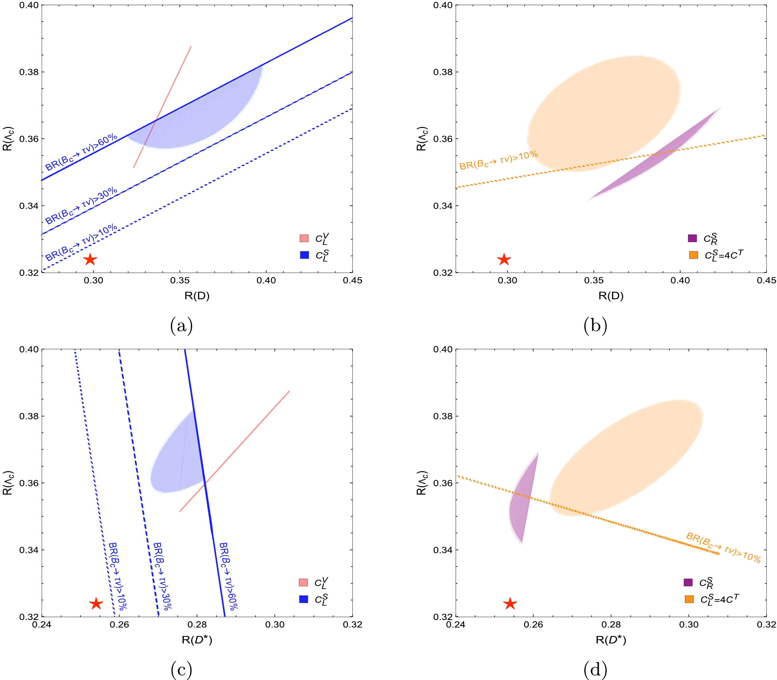

Figure 2.  (color online) Preferred $ 1\sigma $ regions for the four two-dimensional complex scenarios for set $ {\cal{S}}_1 $ in the $ R_{\tau/{\mu,e}}\left(D\right)-R_{\tau/\ell}\left(\Lambda_{c}\right) $$ \text{plane (above) and }R_{\tau/{\mu,e}}\left(D^{*}\right)-R_{\tau/\ell}\left(\Lambda_{c}\right) $ plane (below) for the $ BR\left(B_{c}\to\tau\bar{\nu}_\tau\right)<60\% $. The regions of the plot in the left panel correspond to the $ C_{L}^{V} $ (pink) and $ C_{L}^{S} $ (Blue), whereas the plots on the right panel correspond to $ C_{R}^{S} $ (purple) $ C_{L}^{S}=4C^{T} $(orange). The solid, dashed, dotted lines refer to a constraints on $ {\cal{B}}\left(B^-_{c}\to\tau^-\nu_\tau\right)<60\%,30\% $, and 10%, respectively. The red stars represent SM predictions. In all the figures, we removed the subscripts from the LFU ratios for better visibility.

Similarly, for $ {\cal{S}}_1 $, Fig. 3 shows the preferred $ 1\sigma $ regions for the four two-dimensional complex scenarios in the $ R_{\tau/\mu}\left(J/\psi\right)-R_{\tau/{\mu,e}}\left(D\right) $ and $ R_{\tau/{\mu}}\left(J/\psi\right)-R_{\tau/{\mu,e}}\left(D^{*}\right) $ planes for $ {\cal{B}}(B^-_{c}\to\tau^-\bar{\nu}_\tau)<60\% $bounds. We observe a direct correlation for the WC $ C_{L}^{V} $ and a modest positive correlation for the WCs $ C_{R}^{S} $ scenarios. For $ C_{L}^{S} $ and $ C_{L}^{S}=4C^{T} $ scenarios, we observe a reasonable negative correlation between $ R_{\tau/\mu}\left(J/\psi\right)- R_{\tau/{\mu,e}}\left(D\right) $. Thus, our findings indicate that this correlation pattern can significantly vary for our specific WC scenario. Turning our attention to the correlation between $ R_{\tau/\mu}\left(J/\psi\right) $ and $ R_{\tau/{\mu,e}}\left(D^{*}\right) $, we discover a direct correlation across all WC scenarios. These findings highlight the significance of the interplay between $ R_{\tau/\mu}\left(J/\psi\right) $ and $ R_{\tau/{\mu,e}}\left(D^{*}\right) $ to gain valuable insights into the underlying NP.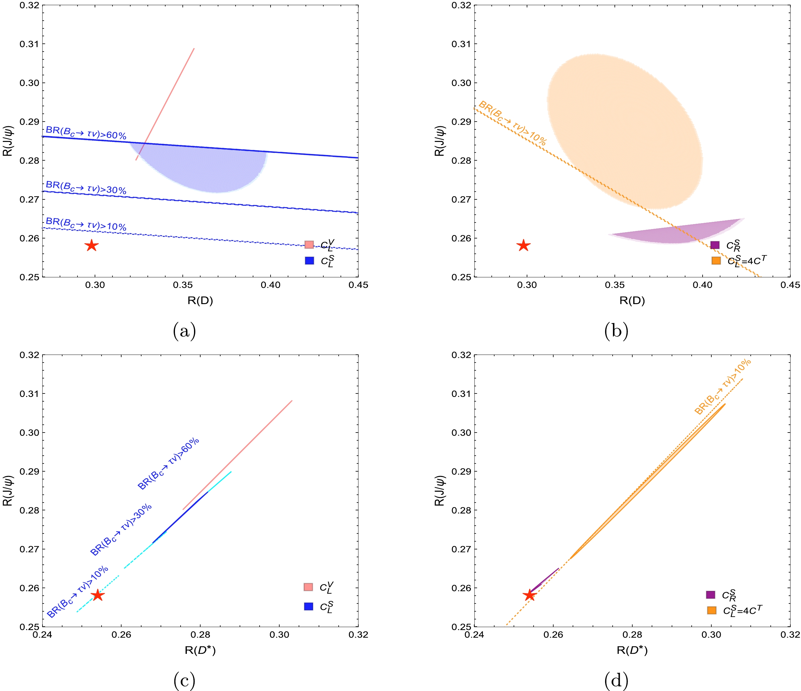

Figure 3.  (color online) Preferred $ 1\sigma $ regions for the four two-dimensional complex scenarios for set $ {\cal{S}}_1 $ in the $ R_{\tau/{\mu,e}}\left(D\right)-R_{\tau/\mu}\left(J/\psi\right) $$ \text{plane (above) and }R_{\tau/{\mu,e}}\left(D^{*}\right)-R_{\tau/{\mu}}\left(J/\psi\right) $ plane (below) for the $ {\cal{B}}(B^-_{c}\to\tau^-\bar{\nu}_\tau)<60\% $. The color coding is the same as in Fig. 2. The red stars represent SM predictions in this case.

Finally, Fig. 4 shows the same results for the $ R_{\tau/\ell}\left(X_{c}\right)- R_{\tau/{\mu,e}}\left(D,D^*\right) $ plane. The correlation patterns between $ R_{\tau/\ell}\left(X_{c}\right) $ and $ R_{\tau/{\mu,e}}\left(D\right) $ or $ R_{\tau/{\mu,e}}\left(D^{*}\right) $ exhibit similar trends as for $ R_{\tau/\ell}\left(\Lambda_{c}\right) $. However, one minor difference occurs in the WC scenario $ C_{L}^{S}=4C^{T} $. In this particular scenario, we observe a moderate positive correlation between $ R_{\tau/\ell}\left(X_{c}\right) $ and $ R_{\tau/{\mu,e}}\left(D^{*}\right) $, compared with the one between $ R_{\tau/\ell}\left(X_{c}\right) $ and $ R_{\tau/{\mu,e}}\left(D\right) $. An additional noteworthy observation is that all the WCs scenarios closely approximate the experimental values of the observable, $ R_{\tau/\ell}\left(X_{c}\right) $, $ R_{\tau/{\mu,e}}\left(D\right) $, and $ R_{\tau/{\mu,e}}\left(D^{*}\right) $, indicating that our results correspond well with the experimental measurements, hence making our findings reliable.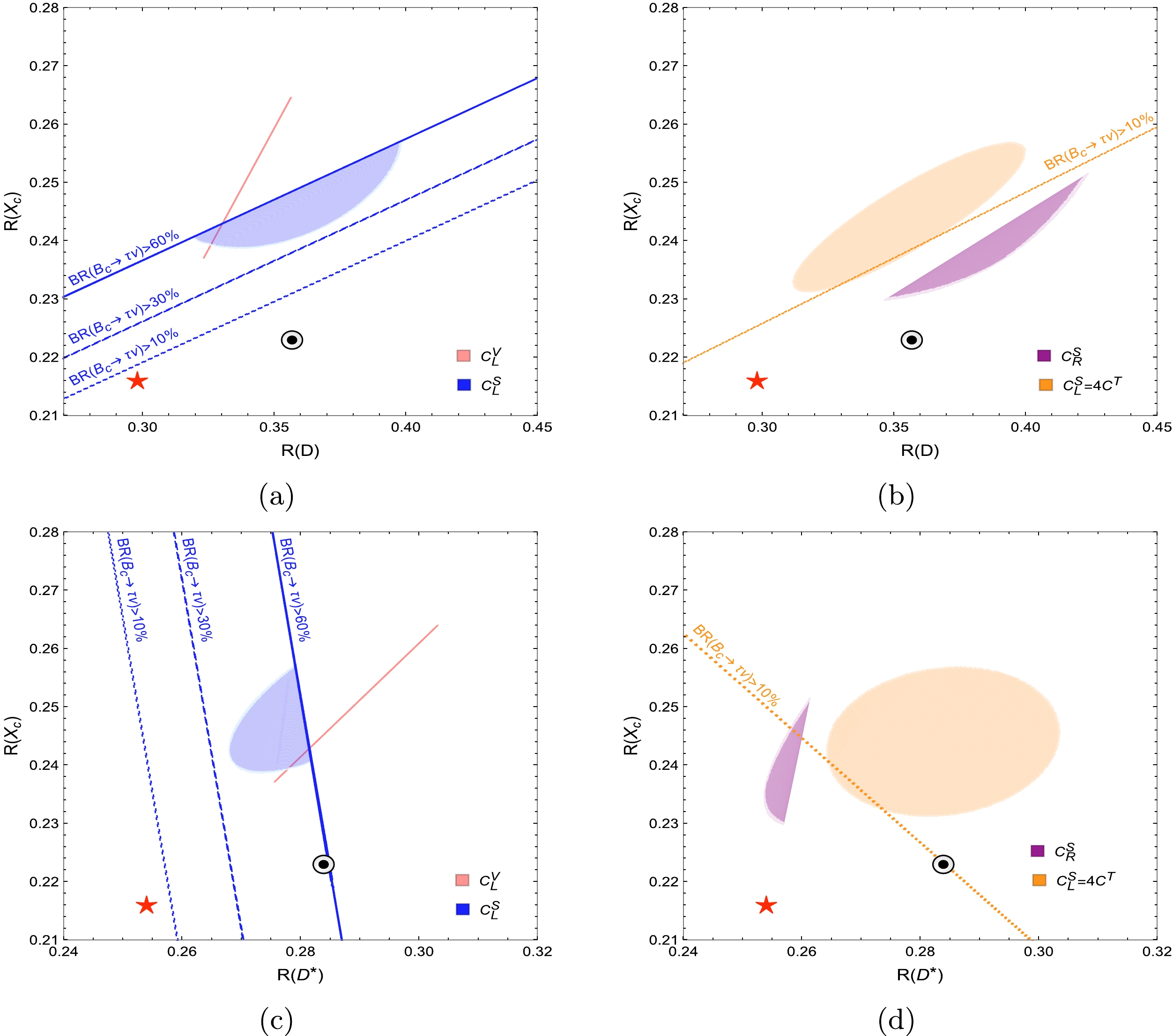

Figure 4.  (color online) Preferred $ 1\sigma $ regions for the four two-dimensional complex scenarios for set $ {\cal{S}}_1 $ in the $ R_{\tau/{\mu,e}}\left(D\right)-R_{\tau/\ell}\left(X_{c}\right) $$ \text{plane (above) and }R_{\tau/{\mu,e}}\left(D^{*}\right)-R_{\tau/\ell}\left(X_{c}\right) $ plane (below) for the $ {\cal{B}}(B^-_{c}\to\tau^-\bar{\nu}_\tau)<60\% $. The color coding is the same as in Fig. 2. The red stars represent SM predictions. The black radio button represents experimental measurements.

In $ B\to D^*\tau \bar{\nu}_{\tau} $ decay, the $ D^* $ meson is unstable, decaying further to $ D\pi $. The geometry of the planes in which $ B\to D^*\tau \bar{\nu}_{\tau} $ and then $ D^*\to D\pi $ decays occur enables us to express the decay rate in terms of various angular observables (see e.g., [59, 100−107]). In this section, we summarize the expressions of various physical observables and discuss the impact of our constrained NP WCs on them. Here, we also study the $ CP $ violation triple product asymmetries, which will hopefully be accessible in ongoing and future flavor physics experiments.

The angular analysis of a four-body $ B\to D^{*} \left(\to D\pi\right)\tau\bar{\nu} $ provides us additional observables. The differential decay rate distribution of the transition process $ B\rightarrow D^{*}\tau\bar{\nu}_\tau $ with $ D^{*}\to D\pi $ on the mass shell has the form [42, 59, 101, 102]

where the lepton-pair invariant mass squared $ q^{2}=\left(p_{\tau}+ p_{\bar{\nu}_\tau}\right)^{2} $, and kinematical variables $ \theta_{\tau}\text{,}\theta_{D}\text{ and }\phi $ are defined as follows. Taking $ D^{*} $ momentum in the B rest frame along the z-axis, D and $ D^{*} $momentum lie in the $ xz$-plane with the positive x-component, and $ \theta_{\tau}\text{ and }\theta_{D} $ are the polar angles between τ and the final D meson in the $ \tau\bar{\nu} $ and $ D\pi $ rest frames, respectively. The angular coefficients ($ I_{i} $) are functions of $ q^{2} $ that encode short- and long-distance physics contributions, and these are given in [59].

Integrating Eq. (31) over different angles, the differential decay rate of $ B\to D^*\left(\to D\pi\right)\tau \bar{\nu}_\tau $ can be expressed as [59, 101, 102]

The decay rate fractions $ R_{A,B} $, $ D^{*} $ polarization fraction $ R_{L,T} $, and forward-backward asymmetry $ A_{FB} $ are given in terms of these angular coefficients $ I's $ as [101]

where

Here, $ \Gamma_{A} $ and $ \Gamma_{B} $ represent partial decay rates with respect to $ \theta_{\ell} $, i.e, angle between the lepton and neutrino in the B rest frame, and $ \Gamma_{L} $ and $ \Gamma_{T} $ represent the rate corresponding to the longitudinal and transverse $ D^{*} $-meson polarization, respectively. In addition to these decay fractions, the other interesting observables are $ A_{3} $, $ A_{4} $, $ A_{5} $, $ A_{6s} $, $ A_{7} $, $ A_{8} $, and $ A_{9} $, and these can be expressed as [101]

Out of these seven observables $ A_{7}, A_{8} $ and $ A_{9} $ are CP-odd, whereas all the others are CP even. After using the values of form factors and other input parameters, and integrating over $ q^2 $, the expressions of the $ I_i's $ in terms of the NP WCs are given in Appendix B.

The inclusion of NP operators and the corresponding WCs in $ b\to c \tau \bar{\nu}_{\tau} $ decays may add a phase that leads to the $ C P$-asymmetries in the corresponding exclusive decays. This additional new phase results in a marked difference between the decay amplitude and its $ C P $ conjugate. However, the possibility of introducing a strong phase due to the interference between the higher $ D^* $ resonances was ruled out by the $ F_{L}\left(D^*\right) $ measurements. In this scenario, some possibilities to investigate the violation of $ C P$-symmetry through triple product asymmetries (TPA) exist. This has been discussed in detail in [108–114], and to make the study self-sufficient, these details are given in Appendix C. The three different transverse asymmetries $ \left(A_{C}^{(i=1,2,3)}\right) $ are [111]

and for the conjugate mode,

Owing to CP even transformation, we are not interested in that. The $ CP $ violating triple products are given as

where the angular coefficients are denoted as $ V's $, whereas the longitudinal and transverse amplitudes are represented as $ A_{L} $ and $ A_{T} $, respectively. For the CP-conjugate decay, the descriptions outlined in Eq. (39) adopt the following formulations:

By employing Eqs. (39) and (40), we define these TPAs as follows [108]:

To obtain a comprehensive understanding of these TPAs, we have expressed the longitudinal, transverse, and mixed amplitudes $ V's $at the central values of the form factors. In addition, to assess the sensitivity of NP, Appendix C summarizes the analytical expressions of these asymmetries in terms of the complex NP WCs.

In this section, we discuss the impact of the constraints of the NP, vector, scalar, and tensor WCs calculated in Sec. III on the above-mentioned physical observables, and we check their NP discriminatory power. Fig. 5 shows the predictions for $ A_{FB} $, $ R_{A,B} $, $ R_{L,T} $, $ A_{3} $, $ A_{4} $, $ A_{5} $, and $ A_{6s} $ as functions of the square of momentum transfer $ \left(q^{2}\right) $. The band in each curve shows the theoretical uncertainties resulting from FFs and other input parameters. The SM value is indciated by the black band, whereas the NP couplings $ C_{L}^{V} $, $ C_{R}^{S} $, $ C_{L}^{S} $, and $ C^{T} $ are indicated in red, orange, pink, and cyan bands, respectively. The corresponding light and dark shades represent $ 1\sigma $ and $ 2\sigma $ intervals. The corresponding numerical values in different $ q^2 $ bins are given in Table 3. We can observe that for $ C_{L}^{S}=4C^{T} $, a significant deviation from the SM value occurs in almost all $ CP $-even angular observables, except for the $ A_{FB} $. Particularly, its effects are constructive (enhancing the SM value) for $ R_{AB},\; A_3,\; A_5 $ and destructive (decreasing the SM value) for the remaining angular observables, where the maximum fall-off is for the $ A_{6s} $. These outcomes make $ C_{L}^{S}=4C^{T} $a promising candidate for investigating physics beyond the SM. In addition, the WC $ C_{L}^{S} $ has the second most significant deviation, particularly for $ A_{FB} $, $ R_{A,B} $, and $ A_{5} $, whereas, the WC $ C_{R}^{S} $ has the same result for the observables $ R_{L,T} $ and $ A_{6s} $. However, the WC $ C_{L}^{V} $ exhibits minimal deviation for all angular observables because it has the same SM Lorentz structure and a small real component. Quantitatively, these findings are given in Table 3. We hope that the experimental measurement of these physical observables will aid in observing particular NP phenomena.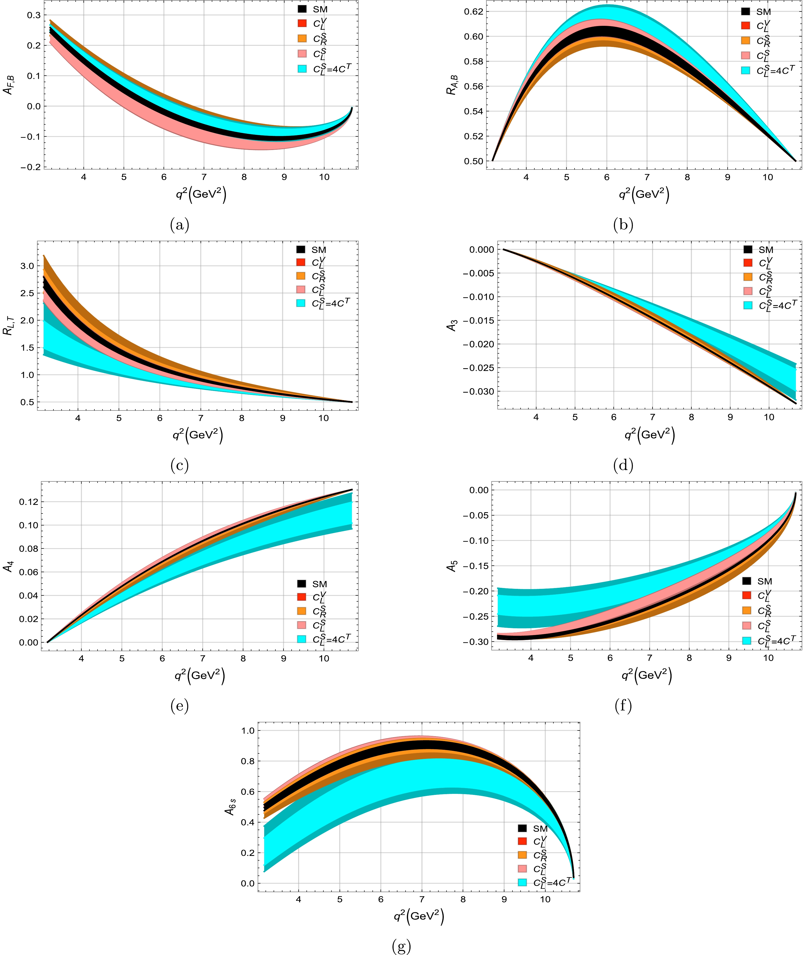

Figure 5.  (color online) $ CP $-even angular observables exhibited for various NP coupling as functions of $ q^{2} $. The width of each curve comes from the theoretical uncertainties in hadronic form factors and quark masses. The $ 1\sigma $ ($ 2\sigma $) intervals (dark color) of the complex NP WCs $ C_{L}^{V} $, $ C_{R}^{S} $, $ C_{L}^{S} $, $ C_{L}^{S}=4C^{T} $, for the set of observables $ {\cal{S}}_1 $ are indicated in red, orange, pink, and cyan, respectively.

Observables	${ {\mathrm{Bins} } /{\mathrm{GeV } }^2 }$	SM	$ C_{L}^{V} $	$ C_{R}^{S} $	$ C_{L}^{S} $	$ C_{L}^{S}=4C^{T} $
$ A_{FB} $	$ \left[3.16,5\right] $	$ 0.144\pm 0.009 $	$ 0.144\pm 0.009 $	$ 0.135\pm 0.054 $	$ 0.108\pm 0.045 $	$ 0.160\pm 0.015 $
	$ \left[5,7\right] $	$ -0.015\pm 0.008 $	$ -0.015\pm 0.008 $	$ -0.027\pm 0.068 $	$ -0.055\pm 0.049 $	$ 0.007\pm 0.027 $
	$ \left[7,9\right] $	$ -0.095\pm 0.007 $	$ -0.095\pm 0.007 $	$ -0.104\pm 0.057 $	$ -0.125\pm 0.038 $	$ -0.075\pm 0.028 $
	$ \left[9,10.69\right] $	$ -0.082\pm 0.004 $	$ -0.082\pm 0.004 $	$ -0.087\pm 0.029 $	$ -0.097\pm 0.019 $	$ -0.072\pm 0.018 $
$ R_{A,B} $	$ \left[3.16,5\right] $	$ 0.559\pm 0.002 $	$ 0.559\pm 0.002 $	$ 0.560\pm 0.008 $	$ 0.562\pm 0.005 $	$ 0.564\pm 0.005 $
	$ \left[5,7\right] $	$ 0.601\pm 0.004 $	$ 0.601\pm 0.004 $	$ 0.603\pm 0.013 $	$ 0.605\pm 0.008 $	$ 0.612\pm 0.012 $
	$ \left[7,9\right] $	$ 0.574\pm 0.003 $	$ 0.574\pm 0.003 $	$ 0.575\pm 0.007 $	$ 0.576\pm 0.005 $	$ 0.584\pm 0.008 $
	$ \left[9,10.69\right] $	$ 0.525\pm 0.001 $	$ 0.525\pm 0.001 $	$ 0.525\pm 0.002 $	$ 0.525\pm 0.001 $	$ 0.529\pm 0.004 $
$ R_{L,T} $	$ \left[3.16,5\right] $	$ 1.953\pm 0.061 $	$ 1.953\pm 0.061 $	$ 1.896\pm 0.430 $	$ 1.794\pm 0.236 $	$ 1.377\pm 0.382 $
	$ \left[5,7\right] $	$ 1.136\pm 0.026 $	$ 1.136\pm 0.026 $	$ 1.105\pm 0.244 $	$ 1.060\pm 0.114 $	$ 0.951\pm 0.140 $
	$ \left[7,9\right] $	$ 0.762\pm 0.011 $	$ 0.762\pm 0.011 $	$ 0.747\pm 0.120 $	$ 0.731\pm 0.048 $	$ 0.702\pm 0.049 $
	$ \left[9,10.69\right] $	$ 0.567\pm 0.003 $	$ 0.567\pm 0.003 $	$ 0.563\pm 0.034 $	$ 0.559\pm 0.012 $	$ 0.554\pm 0.011 $
$ A_{3} $	$ \left[3.16,5\right] $	$ -0.003\pm 0.000 $	$ -0.003\pm 0.000 $	$ -0.003\pm 0.000 $	$ -0.003\pm 0.000 $	$ -0.003\pm 0.000 $
	$ \left[5,7\right] $	$ -0.010\pm 0.000 $	$ -0.010\pm 0.000 $	$ -0.010\pm 0.001 $	$ -0.011\pm 0.000 $	$ -0.009\pm 0.001 $
	$ \left[7,9\right] $	$ -0.019\pm 0.000 $	$ -0.019\pm 0.000 $	$ -0.019\pm 0.001 $	$ -0.020\pm 0.000 $	$ -0.016\pm 0.002 $
	$ \left[9,10.69\right] $	$ -0.028\pm 0.000 $	$ -0.028\pm 0.000 $	$ -0.028\pm 0.001 $	$ -0.028\pm 0.000 $	$ -0.024\pm 0.004 $
$ A_{4} $	$ \left[3.16,5\right] $	$ 0.025\pm 0.000 $	$ 0.025\pm 0.000 $	$ 0.025\pm 0.003 $	$ 0.026\pm 0.001 $	$ 0.020\pm 0.003 $
	$ \left[5,7\right] $	$ 0.068\pm 0.000 $	$ 0.068\pm 0.000 $	$ 0.069\pm 0.006 $	$ 0.071\pm 0.003 $	$ 0.056\pm 0.008 $
	$ \left[7,9\right] $	$ 0.101\pm 0.000 $	$ 0.101\pm 0.000 $	$ 0.102\pm 0.006 $	$ 0.103\pm 0.002 $	$ 0.084\pm 0.013 $
	$ \left[9,10.69\right] $	$ 0.122\pm 0.000 $	$ 0.122\pm 0.000 $	$ 0.122\pm 0.002 $	$ 0.123\pm 0.001 $	$ 0.103\pm 0.016 $
$ A_{5} $	$ \left[3.16,5\right] $	$ -0.289\pm 0.003 $	$ -0.289\pm 0.003 $	$ -0.288\pm 0.004 $	$ -0.280\pm 0.011 $	$ -0.226\pm 0.044 $
	$ \left[5,7\right] $	$ -0.259\pm 0.002 $	$ -0.259\pm 0.002 $	$ -0.255\pm 0.017 $	$ -0.241\pm 0.019 $	$ -0.207\pm 0.038 $
	$ \left[7,9\right] $	$ -0.198\pm 0.002 $	$ -0.198\pm 0.002 $	$ -0.193\pm 0.025 $	$ -0.178\pm 0.022 $	$ -0.161\pm 0.028 $
	$ \left[9,10.69\right] $	$ -0.105\pm 0.001 $	$ -0.105\pm 0.001 $	$ -0.101\pm 0.020 $	$ -0.092\pm 0.014 $	$ -0.086\pm 0.015 $
$ A_{6s} $	$ \left[3.16,5\right] $	$ 0.650\pm 0.023 $	$ 0.650\pm 0.023 $	$ 0.662\pm 0.100 $	$ 0.686\pm 0.062 $	$ 0.371\pm 0.186 $
	$ \left[5,7\right] $	$ 0.862\pm 0.025 $	$ 0.862\pm 0.025 $	$ 0.874\pm 0.110 $	$ 0.893\pm 0.061 $	$ 0.632\pm 0.188 $
	$ \left[7,9\right] $	$ 0.870\pm 0.022 $	$ 0.870\pm 0.022 $	$ 0.877\pm 0.077 $	$ 0.885\pm 0.041 $	$ 0.703\pm 0.165 $
	$ \left[9,10.69\right] $	$ 0.557\pm 0.013 $	$ 0.557\pm 0. $$ 013 $	$ 0.559\pm 0.027 $	$ 0.560\pm 0.017 $	$ 0.472\pm 0.100 $

Table 3.  Numerical values of the abovementioned physical variables at the best-fit-points of various NP couplings in the various $ q^{2} $ bins. The uncertainties result from hadronic form factors and the other input parameters. For distinct WCs $ C_{L}^{V} $, $ C_{R}^{S} $, $ C_{L}^{S} $, $ C_{L}^{S}=4C^{T} $, incorporated the maximum deviations within $ 2\sigma $ intervals in the uncertainties.

In contrast to these physical observables, the values of the $ CP $ odd observables $ A_{7} $ are too small to measure experimentally. Eq. (48) indicates that the expressions of $ I_{8,\; 9} $ are proportional to the imaginary part of the combination of WCs that is real, and hence the asymmetries $ A_{8,\; 9} $ are zero. If we consider the right-handed neutrino operators in the WEH (11), which are not considered in the current study, their interference with the corresponding left-handed operators lead to the non-zero values of $ I_{8,\; 9} $.

Figure 6 shows the predictions for $ \langle A_{T}^{\left(2\right)}\left(q^{2}\right)\rangle $ as functions of $ q^{2} $. The description of the various bands and colors is the same as that of the above angular asymmetries. In the SM, the values of these triple product asymmetries (TPAs) are zero; hence, any non-zero value is attributed to the presence of NP. Specifically, from (49), we observe that $ V_{4}^{0T} $ and $ V_{5}^{T} $ are zero, giving us $ \langle A_{T}^{\left(1\right)}\left(q^{2}\right)\rangle $ and $ \langle A_{T}^{\left(3\right)}\left(q^{2}\right)\rangle $ zero for any NP WCs. The only non-zero contribution is from the $ CP $ violating triple product asymmetry $ \langle A_{T}^{\left(2\right)}\left(q^{2}\right)\rangle $. In this context, for the NP WC $ C_{L}^{V} $, the largest non-zero value or maximum deviation from the SM reaches 0.28 at $ q^{2} $$ =6.5 {\rm{GeV}}^2 $ when $ C_{L}^{V} $$=-1.5 \pm 0.9 {\rm i}$. This data point falls within the $ 2\sigma $ interval. In a $ 1\sigma $ interval, the maximum deviation is 0.23, occurring at $ q^{2}=6.5{\rm{GeV}}^2 $ for $ C_{L}^{V} $ of $-1 - 1.05 {\rm i}$ and $-1.17 + 1.06{\rm i}$. The other non-zero deviation from the SM result is for $ C_{L}^{S}=4C^{T} $; however, the maximum value here is 0.008 at $ q^{2}=6.5{\rm{GeV}}^2 $, corresponding to WC $ C_{L}^{S} $ of $-0.08+0.33{\rm i}$ and $-0.11+0.34{\rm i}$; however, this is too small to be measured experimentally. Similarly, for the WCs $ C_{R}^{S} $ and $ C_{L}^{S} $, this asymmetry remains zero in the entire $ q^2 $ range. Therefore, we can conclude that experimental observation of $ \langle A_{T}^{\left(2\right)}\left(q^{2}\right)\rangle $ will make the new vector type operators an important candidate to hunt for the NP in flavor sector.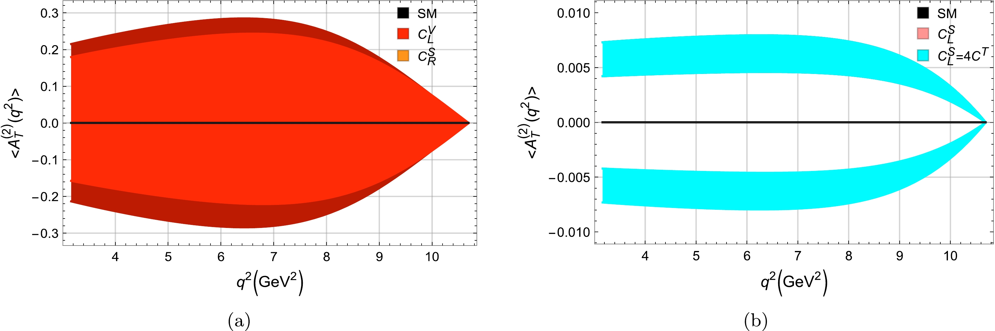

Figure 6.  (color online) $ CP $-violating TPAs exhibited for various NP couplings as functions of $ q^{2} $. The width of each curve results from the theoretical uncertainties in hadronic form factors and quark masses. The $ 1\sigma $ sigma ($ 2\sigma $) intervals in color (dark color) of the complex coupling WCs $ C_{L}^{V} $, $ C_{R}^{S} $, $ C_{L}^{S} $, $ C_{L}^{S}=4C^{T} $, for the set of observables $ {\cal{S}}_1 $ are in red, orange, pink, and cyan, respectively.

The Standard Model (SM) elegantly explains most experimentally observed phenomena, and no new particles beyond those present in the SM have been discovered thus far. However, some deviations occur from the SM predictions observed in flavor-changing-charged-current (FCCC) transitions involving the third generation of leptons i.e., $ b\to c\tau \bar{\nu}_\tau $. In this scenario, it is important to explain how to study these indirect the signatures of new physics (NP).

In this paper, we have analyzed anomalies observed in $ b\to c\tau \bar{\nu}_\tau $ decays by including new vector, scalar, and tensor operators in the SM effective Hamiltonian. We assume the corresponding Wilson coefficients (WCs) to be complex and also we consider the neutrinos to be left-handed. Our study is composed of two sets of observables. In the first set $ \left({\cal{S}}_1\right) $, we include $ R_{\tau/{\mu,e}}\left(D\right), R_{\tau/{\mu,e}}\left(D^*\right), F_{L}\left(D^*\right) $, and $ P_{\tau}\left(D^*\right) $, whereas in the second one $ \left({\cal{S}}_2\right) $, we include two more experimentally measured observables, $ R_{\tau/\mu}(J/\psi) $ and $ R_{\tau/\ell}(X_c) $. For these two sets, we have estimated the best-fit points, p-value, $ \chi_{{\rm{SM}}}^{2} $, $ {\rm{pull}}_{{\rm{SM}}} $, and $ 1,2\sigma $ deviations for these complex WCs. As the branching ratio of $ B_c\to \tau \bar{\nu}_\tau $ is not yet measured, we have shown our results for the 60%, 30%, and 10% limits on it. We find that the NP WCs $ C^{V}_{L} $ and $ C^S_{R} $ are not sensitive to these bounds, whereas the $ C^S_{L} $ the p-value is maximum for 60% limits. The value of BFPs and the p-value significantly change for $ {\cal{S}}_2 $. This is attributed to the large errors in the experimental measurements of $ R_{\tau/\mu}\left(J/\psi\right) $ and $ R_{\tau/\ell}\left(X_c\right) $. We expect that when these measurements are refined in the future, we will have better control over the parametric space of these new WCs.

Because of the same quark level transition, a strong theoretical correlation exists between $ R_{\tau/{\mu,e}}\left(D^{(*)}\right) $ and $ R_{\tau/{\mu,e}}\left(\Lambda_c\right) $. Using the updated values of different input parameters and the experimental measurements for $ R_{\tau/{\mu,e}}\left(D^{(*)}\right) $, the updated sum-rule was derived in [66]. We validate the sum rule in our case and find that the remainder is $ <10^{-3} $. Similarly, we derive similar sum rules for $ R_{\tau/\mu}\left(J/\psi\right) $ and $ R_{\tau/\ell}\left(X_c\right) $ relating them with $ R_{\tau/{\mu,e}}\left(D^{(*)}\right) $. We observe that in $ R_{\tau/\mu}\left(J/\psi\right) $ the maximum contribution comes from the LFU ratio of $ D^* $; hence, large deviations in the $ R_{\tau/{\mu,e}}\left(D^{*}\right) $ will strongly impact this ratio. Using the best-fit values of our complex WCs, and the latest measurements of the $ R_{\tau/{\mu,e}}\left(D^{(*)}\right) $, we calculate $R_{\tau/\mu}\left(J/\psi\right) = 0.289$ and $ R_{\tau/\ell}\left(X_c\right)=0.248 $. In addition, we plot the correlation of $ R_{D} $ and $ R_{D^*} $ with other observables and hope that the correlation of $ R_{\tau/{\mu,e}}\left(D^{(*)}\right) $ with other physical observables will aid us in discriminating between different NP scenarios.

Furthermore, we investigate the effects of these NP WCs on different angular asymmetries and the $ CP $-violation triple product in $ B\to D^*\tau \bar{\nu}_\tau $ decays. We find that the most promising effects on the different angular asymmetries are attributed to the NP WC $ C_{L}^{S}=4C^{T} $. We know that the $ CP $-triple product in the SM is zero, and any non-zero value would hint towards NP. We find that for the vector-like new operators, the maximum value of $ \langle A_{T}^{\left(2\right)}\left(q^{2}\right)\rangle = $ 0.28. We hope our results can be tested at the LHCb and future high-energy experiments.

The authors would like to thank Prof. Monika Blanke and Dr. Teppei Kitahara for helping us understand their research and suggesting improvements in our code, and we appreciate this kind gesture. MJA and SS would like to thank Wang Yu-Ming for reading the manuscript and suggesting some important references.

No Data associated in the manuscript.

We determine $ \chi^2 $ to test the hypothesis about the distribution of observables in distinct effective operators. This enables us to quantify the discrepancy between the theoretical and experimental data used to fit. $ \chi^{2} $ is expressed as [115, 116]

where $N_{\rm obs}$ is the number of observables, $O_{i}^{\rm exp.}$ are the data from experiments, and $O_{i}^{\rm th}$ are the theoretical parameters of the observables, which are complex functions of scalar and vector WCs $ C_{M}^{X} $ $ (X=S,V) $ and $ (M=L,R) $. The covariance matrix is the sum of theoretical and experimental uncertainties and consider the experimental correlation between $ R_{\tau/{\mu,e}}(D) $ and $ R_{\tau/{\mu,e}}(D^{*}) $ in terms of ${\rm pull}$, calculated as

where the correlation value ρ taking from the HFLAV is –0.37. First, we determine the number of degrees of freedom ($\rm dof$) we have, which is equal to $N_{\rm dof}=N_{\rm obs}-N_{\rm par}$, where $ N_{\rm par} $ is the number of parameters to be fitted for each parameter. For complex WCs, as we have in our case, we have $N_{\rm par}=2$ and $N_{\rm obs}=4$ and 6 for the sets of observables $ {\cal{S}}_1 $ and $ {\cal{S}}_2 $. In the second step, we obtain the minimum value of $ \chi^{2} $ for each parameter to acquire best fit points (BFPs). Third, we utilize the value of $ \chi^{2} $ to obtain the $p\text{-}{\rm{value}}$. The $p\text{-}{\rm{value}}$ for the hypothesis can be calculated as [115, 116]

where $ f(z;n_{d}) $ is the $ \chi^{2} $ probability distribution function, and $ n_{d} $ is the number of dof. The $ p $-values quantify the consistency between data and the hypothesis of the NP scenario. Finally, we estimate the value of $ {\rm{pull}} $ from the SM in units of standard deviation (σ) determined by

where $ \chi_{\rm{{\rm{SM}}}}^{2}=\chi^{2}(0) $.

After incorporating the form factors and other input parameters, the integration over $ q^2 $ leads to the expressions of the angular coefficients $ \left(\times 10^{-16}\right) $ in terms of our complex NP WCs, i.e.,

Defining $ \theta_{D} $ and $ \theta_{\tau} $ as angles between the D meson (that originates from the cascade decay of $ D^*\to D\pi $ mesons) and that of τ with the decaying B-meson, respectively. Additionally, the angle φ indicates the angular difference between the decay plane of $ D^{\ast} $ and the plane defined by the momenta of the τ lepton and the corresponding $ \left(\nu_\tau\right) $ neutrino.

The relevant triple products are computed through the integration of the complete decay distribution across distinct ranges of the polar angles $ \theta_{D} $ and $ \theta_{\tau} $. This process yields the following triple products as the outcomes of interest [108, 110–114].

and

The coefficients $ A_{C}^{\left(i\right)} $of $ \cos\phi $ and $ \cos2\phi $ are $ C P$−even, and the coefficients $ A_{C}^{\left(i\right)} $of $ \sin\phi $ and $ \sin2\phi $ are CP-odd, under the $ C P $ transformation. The expressions of V's in terms of the NP WCs are

From Ref. [111], we observe that $ V_{4}^{0T} = \sqrt{2}\left(1-\dfrac{m_{\tau}^2}{q^2} \right) \Im\left[{\cal{A}}_{\perp}^*{\cal{A}}_{0}\right] $, which after integrating over $ q^2 $ is proportional to $ \Im\left|1+C_{L}^{V}\right|^2 $, and hence it is zero.