Observational appearance and extra photon rings of an asymmetric thin-shell wormhole with a Bardeen profile

The initial direct detection of the gravitational-wave signal by the Laser Interferometer Gravitational Wave Observatory (LIGO) marked a significant milestone, providing compelling evidence for the existence of a binary stellar-mass black hole (BH) system [1–3]. Moreover, the groundbreaking observations conducted by the Event Horizon Telescope (EHT) further support the existence of supermassive BHs in both ${\rm{M}} 87^*$ and Sagittarius ${\rm{A}}^*$ [4–15]. The BH image exhibits a central dark region encircled by a luminous ring, arising from the interaction between light rays and the photon sphere (also referred to as the critical curve) of the BH [16]. The region enclosed by the critical curve, commonly referred to as the BH shadow, is indeed situated in the central area of the image [17]. The BH image provides comprehensive information regarding the jet and surrounding matter, enabling us to investigate essential physical properties of the BH, including its mass, rotation, and charge. For the Schwarzschild BH, Synge and Luminet studied the angular radius for the photon capture region [18, 19]. For the Kerr BH, Bardeen studied the deformation of the BH shadow due to the dragging effect of the spin [20–22]. Recently, there has been a significant surge in the investigation of BH shadows within the realm of modified gravity theories [23–52].

However, there still exists some uncertainty regarding the definitive identification of the ultracompact objects (UCOs) located at the center of ${\rm{M}} 87^*$ and Sagittarius ${\rm{A}} ^*$ as BHs within the framework of general relativity (GR). Although the results obtained from the EHT primarily focus on BHs in GR, they do not completely exclude the possibility of BHs in modified gravity theories or other UCOs. In fact, certain UCOs have the potential to create a shadow resembling that of a BH [53–59]. Therefore, it is imperative to develop a methodology capable of discerning BHs from other UCOs, such as wormholes [60–73] and boson stars [74–77]. As an innovative attempt, Wang et al. studied the optical appearance of an asymmetric thin-shell wormhole (ATSW), demonstrating that the shadow of the ATSW exhibits a smaller size compared to that generated by a BH [60]. This finding presents a promising avenue for directly observing wormholes. Subsequently, the researchers focused on analyzing the double shadows cast by ATSWs, presenting a novel radioastronomical observation approach to differentiate UCOs from BHs [61–63]. Moreover, the optical appearance and extra photon rings of the Schwarzschild ATSW was studied in [64]. The optical appearance and extra photon rings of an ATSW with a Hayward profile were studied in [65], while the optical appearance of an infalling star within an ATSW was examined in the research carried out by [66]. Olmo et al. [70] studied the observational appearances of BHs and traversable wormholes, as well as the Lyapunov exponents of the unstable circular orbit for the photon. Bronnikov et al. [71] calculated the quasinormal modes and shadows for different examples of the parametrization of the wormhole metrics.

It is well known that the singularity theorem [78, 79], established by Penrose and Hawking, asserts that within the framework of GR, if the strong energy conditions are satisfied and the global hyperbolicity exists, then the BH will inevitably confront the issue of singularity. The singularity of spacetime is characterized by the divergence of curvature and density to infinity, leading to a complete breakdown in the predictive capacity of physical laws. The singularity of spacetime is widely believed to be a manifestation of the incompleteness inherent in GR, which could potentially be resolved through the incorporation of the quantum gravity theory. However, Bardeen proposed the regular BH solution, which circumvents the BH singularity [80]. In [81–84], Ayon-Beato and Garcia revealed that the physical source of the Bardeen BH is a nonlinear magnetic monopole. Furthermore, as an additional regular BH solution, the Hayward BH was discovered in [85]. In our previous work [86], we observed a correlation between changes in magnetic charge g and the characteristics of the BH shadow. Specifically, an increase in magnetic charge g leads to a reduction in both the size of the shadow region and its associated bright rings when considering a Bardeen BH surrounded by a thin disk accretion. In this work, we focus on examining the characteristics of optical appearance projected by the ATSW with a Bardeen profile. On the one hand, the observational appearance of the Schwarzschild ATSW was studied in [64], prompting our interest in exploring whether variations in magnetic charge g would induce corresponding alterations in the observed characteristics of an ATSW with a Bardeen profile, similar to those found in the case of the Bardeen BH. On the other hand, we wanted to investigate whether it is possible to distinguish between ATSWs and BHs based on the characteristics of their shadows, thus providing a viable approach for studying strong gravitational systems from an observational perspective.

The organization of this paper is as follows: In Sect. II, the ATSW with a Bardeen profile is constructed and its geodesic is studied. Next, the light deflection and trajectory of the light ray in the ATSW spacetime are calculated. In Sect. III, the transfer functions and the observational appearances of both the BH and ATSW in two emission models are studied. Our conclusions are given in Sect. IV. In this paper, we adopt units $G=c=1$.

In this section, we use Visser's cut-and-paste method to construct an ATSW with a Bardeen profile [87]. The ATSW consisted of two spacetimes ${\cal{M}}_{1}$ and ${\cal{M}}_{2}$ with different mass parameters $M_1$ and $M_2$, connected by a thin shell (i.e., the "throat"). The ATSW can be represented by the manifold ${\cal{M}}$, which is defined as ${\cal{M}} \equiv {\cal{M}}_{1} \cup {\cal{M}}_{2}$, that is,

For the Bardeen case, metric $f_i\left(r_i\right)$ can be written as [80]

where $M_i$ denotes the mass parameter, and g is the magnetic charge. R denotes the position of the thin shell and satisfies $R>\max \left\{r_{h_{1}}, r_{h_{2}}\right\}$, where $r_{h_{1}}$ and $r_{h_{2}}$ denote the event horizon radii of BHs. Considering that the gravitational interaction is the only force acting on photons as they pass through the thin shell, the 4-momentum $p^a$ of the photon remains constant. In spacetime ${\cal{M}}$, we have $g_{\mu\nu}^{{\cal{M}}_{1}}(R) = g_{\mu\nu}^{{\cal{M}}_{2}}(R)$ due to the continuity of the metric [60]. This system has two conserved quantities, namely, $p_{t_i}=-E_i$ and $p_{\phi_i}=L_i$, when the photon moves along the geodesic and satisfies the motion equation

in which $p_i^{r_i}={{\rm d} x^{r_i}}/{{\rm d} \lambda}$ is the 4-momentum of the photon, where λ is the affine parameter. From Eq. (3), we obtain

Here, symbols $+$ and $-$ represent the outgoing and incoming directions, respectively. $b_i$ is an impact parameter, which is given by $b_i = |L_i| / E_i$. Using Eq. (4), one can obtain that the effective potential $V_{i}(r_{i})$ of the ATSW with a Bardeen profile is

Moreover, for photons occupying the unstable circular orbit, one can obtain that

where $b_{c}$ denotes the critical impact parameter, and $r_{ph}$ denotes the photon sphere radius. When the event horizon is obscured by the photon sphere, it is necessary to find a way to distinguish the ATSW from the BH. Given that an observer is located in spacetime ${\cal{M}}_{1}$ with mass parameter $M_1=1$, we set $M_2=k$ for spacetime ${\cal{M}}_{1}$. Terms of k and R must satisfy the following condition [60, 64]:

In fact, the subsequent discussion and result remain consistent for any $1<k<\dfrac{R}{2}$. Following the approach adopted in previous studies [64, 65], we set $M_2=k=1.2$. In the distinct spacetimes ${\cal{M}}_{1}$ and ${\cal{M}}_{2}$, one can obtain the relationship of impact parameters $b_{1}$ and $b_{2}$ as follows [60]:

Given that $M_1=1$ and $M_2=1.2$, we use Eq. (6) to calculate photon sphere radius $r_{ph_i}$ and critical parameter $b_{c_{i}}$ for different values of magnetic charge g, as presented in Table 1. The result shows that an increase in magnetic charge g leads to a decrease in both photon sphere radius $r_{ph}$ and critical impact parameter $b_{c_{i}}$, which implies that an increase in g causes an inward contraction of the photon sphere. Note that $g=0$ corresponds to the Schwarzschild ATSW.

g	0	$0.1$	$0.3$	$0.5$	$0.7$
$b_{c_{1}}$	$5.19615$	$5.18745$	$5.11484$	$4.9488$	$4.58839$
$r_{ph_{1}}$	3	$2.99162$	$2.92088$	$2.75252$	$2.3132$
$b_{c_{2}}$	$6.23538$	$6.22814$	$6.16853$	$6.0386$	$5.80418$
$r_{ph_{2}}$	$3.6$	$3.59303$	$3.53519$	$3.40605$	$3.15773$

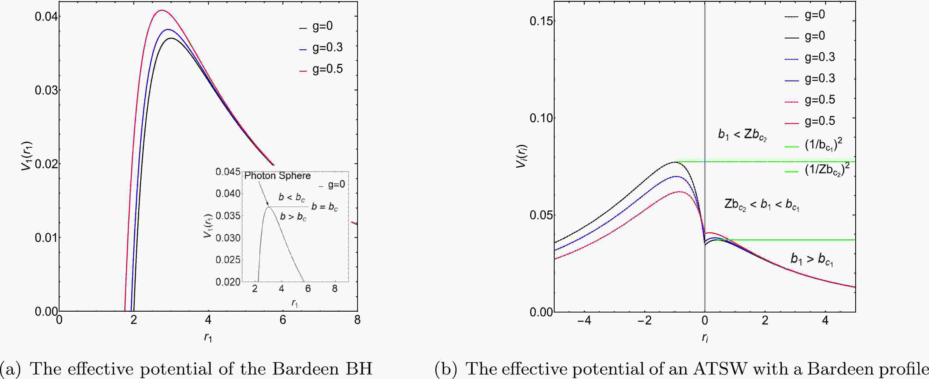
Table 1.  Critical impact parameters and photon sphere radii for the ATSW with a Bardeen profile. We consider different magnetic charges g = $0,\,0.1,\,0.3,\,0.5,\,0.7$. For spacetime ${\cal{M}}_1$, we set $M_1=1$, while for spacetime ${\cal{M}}_2$, we set $M_2=1.2$.

The effective potentials of the Bardeen BH and ATSW with a Bardeen profile are shown in Fig. 1. For the effective potentials of the BH in Fig. 1, three distinct cases of trajectories of photons [16] can be observed in the illustration positioned in the bottom right corner of Fig. 1(a). When $b < b_{c}$, the photon falls into the BH. When $b = b_{c}$, the photon has a periodic circular motion around the BH. When $b > b_{c}$, the trajectory of the photon is deflected due to the gravitational force. In addition, Fig. 1(a) shows that the peak of the effective potential exhibits an upward trend as parameter γ increases.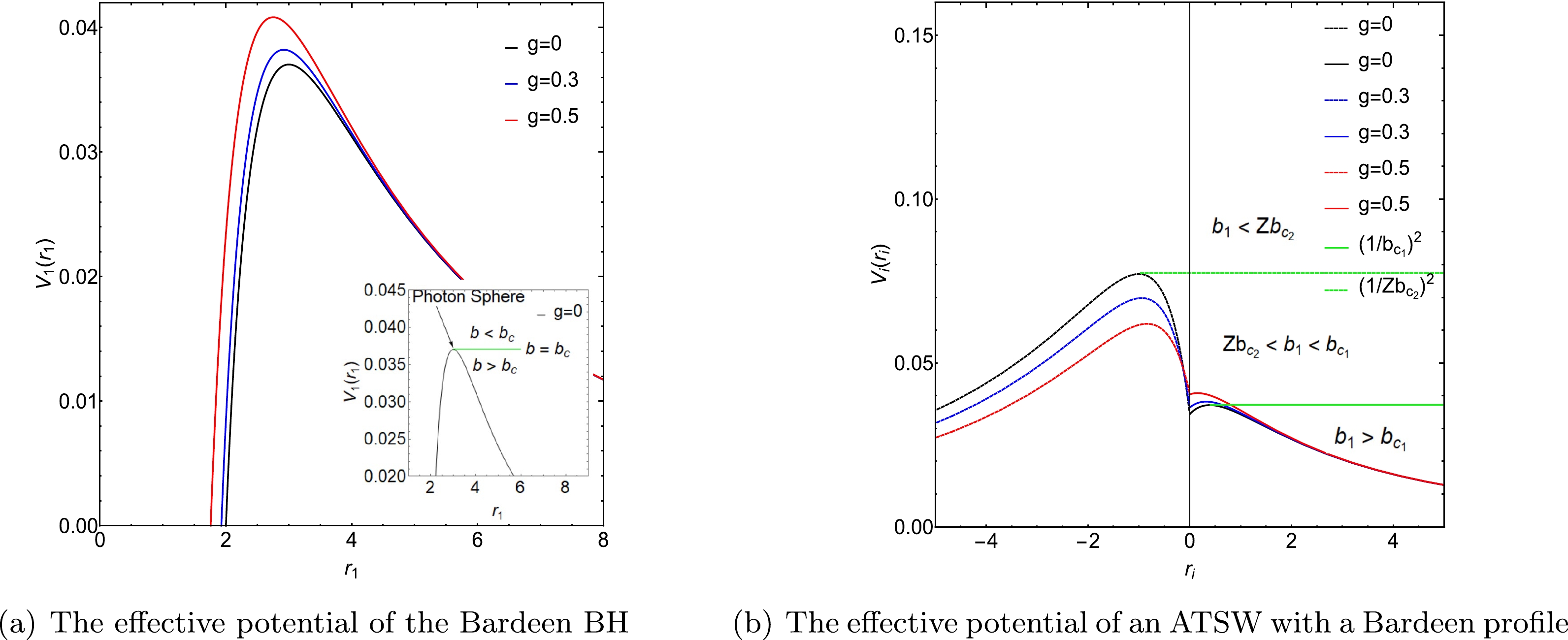

Figure 1.  (color online) Effective potentials for the Bardeen BH and ATSW with a Bardeen profile. We consider different magnetic charges g: $0,\,0.3,\,0.5$. The BH case is shown in the left panel, while the ATSW case is shown in the right panel. For the ATSW case, the effective potentials in spacetimes ${\cal{M}}_1$ and ${\cal{M}}_2$ are represented by the solid and dashed lines, respectively. For magnetic charge $g=0$, one can obtain $b_{c_1}=5.1965$ (the green line) and $Zb_{c_2}=3.6$ (the green dashed line). Here, we take $M_1=1,\, M_2=1.2$, and $R=2.6$.

For the effective potentials of the ATSW in Fig. 1(b), $V_{2}(r_{2})$ in spacetime ${\cal{M}}_2$ is scaled by a factor of $Z^2$. Given a specific impact parameter, $b_1$, three cases of trajectories of photons can be observed. Considering the case of $g=0$, corresponding to the black and green lines in Fig. 1(b), when $b_1<Zb_{c_2}=3.6001$, the photon in spacetime ${\cal{M}}_1$ drops into spacetime ${\cal{M}}_2$ and then moves to infinity in spacetime ${\cal{M}}_2$. When $Zb_{c_2}<b_1<b_{c_1}= 5.19615$, the photon in spacetime ${\cal{M}}_1$ reaches the turning point in spacetime ${\cal{M}}_2$ and then returns to spacetime ${\cal{M}}_1$. When $b_1>b_{c_1}$, the photon in spacetime ${\cal{M}}_1$ reaches the turning point in spacetime ${\cal{M}}_1$ and then returns to infinity in spacetime ${\cal{M}}_1$.

To investigate the optical appearance of the ATSW with a Bardeen profile, we performed calculations to determine the trajectory and deflection angle of photons as they propagate within the spacetime of the ATSW. Using Eq. (3), one can obtain the trajectory of the photon as follows:

To streamline the calculation process, we introduce $x \equiv 1/r$ and subsequently derive the motion equation of photon as

In the case of $b_1<Zb_{c_2}$, the photon will drop into spacetime ${\cal{M}}_2$ and then move to infinity in spacetime ${\cal{M}}_2$. In this scenario, the consideration of the deflection angle of the photon is unnecessary. When $b_1>b_{c_1}$, the photon will remain within spacetime ${\cal{M}}_1$. The turning point in spacetime ${\cal{M}}_1$ can be determined by the minimum positive root of $G_1(x_1)=0$, which is represented by $x_1^{\min}$. With Eq. (10), the total change of the azimuth angle, i.e., the deflection angle, for the photon in spacetime ${\cal{M}}_1$ is calculated by

If $Zb_{c_2}<b_1<b_{c_1}$, the photon will reach the turning point in spacetime ${\cal{M}}_2$ and return to spacetime ${\cal{M}}_1$. In spacetime ${\cal{M}}_1$, the deflection angle for the photon is calculated by

In spacetime ${\cal{M}}_2$, the turning point can be determined by the maximum positive root of $G_2(x_2)=0$, which is represented by $x_2^{\max}$. In addition, impact parameter $b_2$ can be obtained by Eq. (8). Hence, in spacetime ${\cal{M}}_2$, the deflection angle for the photon is calculated by

With Eqs. (11)−(13), the trajectories of photons in the ATSW spacetime are plotted in Fig. 2. Considering $g=$ 0.3 as an example, the impact parameter satisfies the condition $Zb_{c_2}<b_1<b_{c_1}$, as shown in Figs. 2(d), 2(e), and 2(f). For the photon that originates from infinity in spacetime ${\cal{M}}_{1}$, we find that as impact parameter $b_1$ decreases, the trajectory of the photon in spacetime ${\cal{M}}_{2}$ becomes longer. In Fig. 2, from the left column (Fig. 2(a), 2(d), and 2(g)) and the right column (Fig. 2(b), 2(e), and 2(h)), it can be found that as magnetic parameter g increases, $b_{c_1}$ decreases, while $Zb_{c_2}$ increases.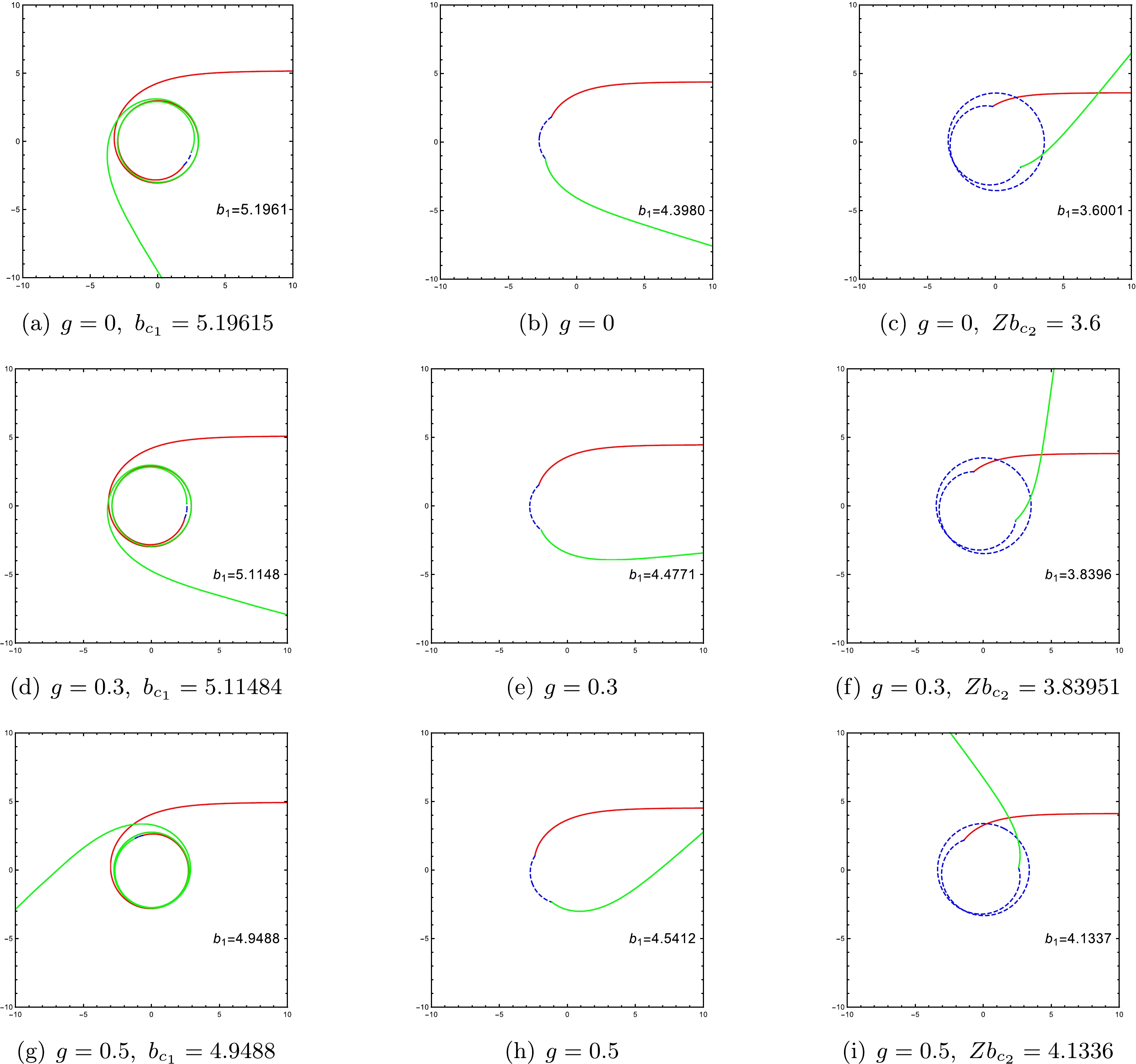

Figure 2.  (color online) Trajectories of light rays with impact parameter $Z b_{c_2}<$ $b_1<b_{c_1}$ for the ATSW with a Bardeen profile. We consider different magnetic charges g: $0,\,0.3,\,0.5$. The red solid lines represent the incoming photons in spacetime ${\cal{M}}_{1}$, the blue dashed lines represent the photons that move in spacetime ${\cal{M}}_{2}$, and the green solid lines represent the outgoing photons in spacetime ${\cal{M}}_{1}$. Here, we take $M_1=1, M_2=1.2$, and $R=2.6$.

For an incoming photon with a specific impact parameter, the unique reflection mechanism of the ATSW makes its observable appearance different from that of the BH. We consider that an optically and geometrically thin disk encircles the ATSW with a Bardeen profile. With two emission models, we compare the observational appearances of the ATSW and the BH.

First, we introduce the total orbit number of the photon, which quantifies the total number of cycles that the photon completes around the BH, that is,

As the deflection angle depends on the impact parameter, it is natural for the total number of orbits to also be a function of the impact parameter. For a BH with a fixed equatorial plane, the observer is positioned at infinity on its North Pole and the light source is placed at infinity on its South Pole. Based on the value of the total number of orbits n, the light near the BH can be classified into the following three types [16]:

● Direct emission: $n < 3/4$. The photon intersects with the equatorial plane only once;

● Lensing ring: $3/4 < n < 5/4$. The photon crosses the equatorial plane twice;

● Photon ring: $n > 5/4$. The photon crosses the equatorial plane at least three times.

For the optical appearance of the ATSW, we consider that the observer in spacetime ${\cal{M}}_{1}$ is positioned at the North Pole. For the photon with impact parameter $Z b_{c_2}<b_1<b_{c_1}$ that originates from spacetime ${\cal{M}}_{1}$, it will drop into spacetime ${\cal{M}}_{2}$. For the ATSW case, the orbit number is redefined as follows [64]:

where $n_{2}$ and $n_{3}$ are the additional orbit functions for the ATSW, which correspond to the additional photon rings.

In Fig. 3, orbit number $n_{1,2,3}$ is shown as a function of impact parameter $b_1$ for a photon. For orbit number $n_{1}$ in Fig. 3(a), one can find that the orbit number $n_{1}$ of the ATSW is the similar to that of a BH. In this case, the photon remains in spacetime ${\cal{M}}_{1}$. When the photon drops into spacetime ${\cal{M}}_{2}$ and returns to spacetime ${\cal{M}}_{1}$, if $n_{2}<3/4$ (solid lines in Fig. 3(b)) and $n_{3}>3/4$ (dashed lines in Fig. 3(b)), it will finally intersect with the accretion disk on the back side. If $n_{2}<5/4$ and $n_{3}>5/4$, the photon will finally intersect with the accretion disk on the front side. In addition, it can be found from Fig. 3(b) that with an increase in magnetic charge g, the range of impact parameter $b_1$ decreases. This result implies that as magnetic charge g increases, these additional photon rings will contract towards the inner region of the ATSW shadow. This result is consistent with the results presented in Table 1 and Fig. 2.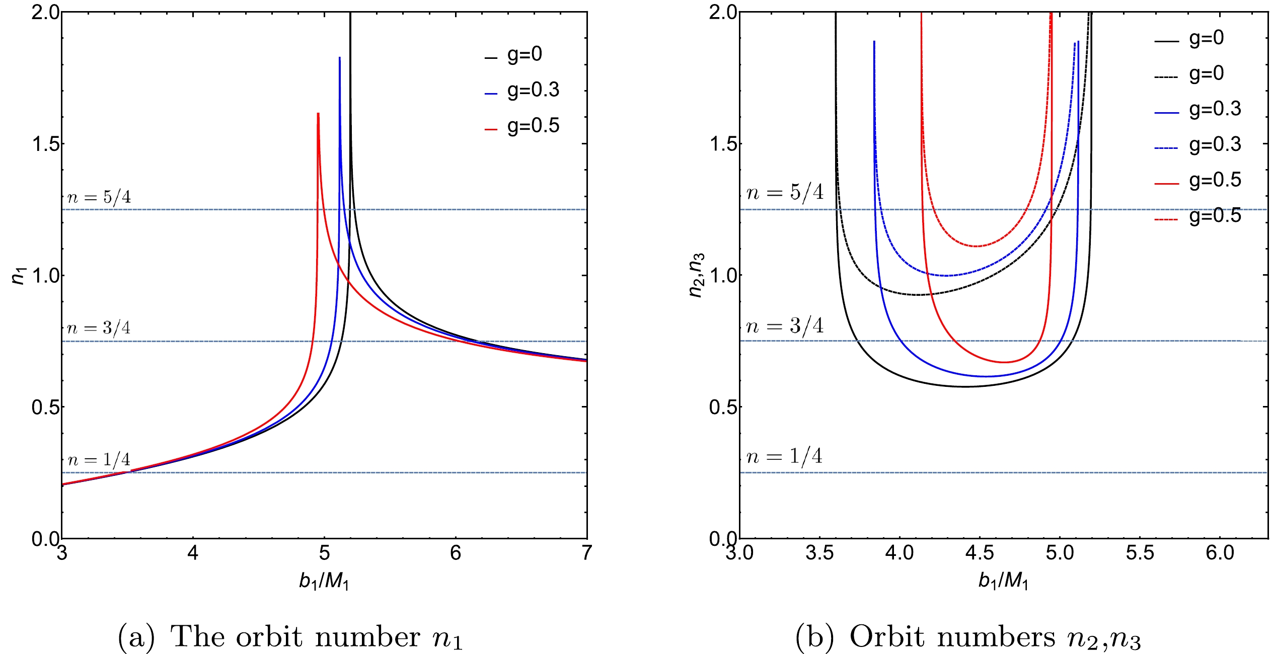

Figure 3.  (color online) Orbit number of the photons around the ATSW with a Bardeen profile. We consider different magnetic charges: $g=0$ (black lines), $g=0.3$ (blue lines), and $g=0.5$ (red lines). Orbit number $n_2$ is shown in the left panel, while orbit numbers $n_2$ (solid lines) and $n_3$ (dashed lines) are shown in the right panel. $M_1=1, M_2=1.2$, and $R=2.6$.

We consider that the emission originates from an optically and geometrically thin accretion disk around the ATSW, which is located in spacetime ${\cal{M}}_{1}$. Assuming that a static observer in spacetime ${\cal{M}}_{1}$ is located at the North Pole, and the accretion disk is situated in the equatorial plane. The emission from the accretion disk is isotropic for the static observer in the rest frame. Considering the spherical symmetry of spacetime ${\cal{M}}_{1}$, the emitted specific intensity depends on the radial coordinate as $I^{\rm{em}}_\nu(r)$, where ν represents the emission frequency in the static frame. Then, we have

The observed specific intensity reads

One can integrate Eq. (19) to obtain the total observed intensity for each intersection as follows:

where $I^{{\rm{em}}}(r)=\int I_\nu^{{\rm{em}}} {\rm d} \nu$ denotes the total emitted intensity. Then, one can calculate the total observed intensity for all intersections, that is,

in which transfer function $r_{n}(b_1)$ denotes the radial coordinate of the n-th intersection between the photon with impact parameter $b_1$ and the accretion disk. In addition, the derivative of the transfer function (i.e., ${\rm{d}}r/{\rm{d}}b_1$) can be defined as the demagnification factor. In fact, the "direct emission" (the redshift of the source profile) is provided by the transfer function ($n=1$), while the "lensing ring" is provided by the second transfer function ($n=2$), and the "photon ring" is provided by third transfer function ($n=3$).

The transfer functions as functions of the impact parameter are shown in Fig. 4, where we consider various magnetic charges. Fig. 4(a) shows the transfer functions with magnetic charge $g=0.3$. The results indicate that the first transfer function produces a "direct image" with a small demagnification factor, indicating the redshift of the source profile. The second transfer function generates the "lensing ring," which has a large demagnification factor and represents the reduced image of the back side of the disk. The third transfer function generates the "photon ring," exhibiting an even higher demagnification factor and resulting in a highly reduced image of the front side of the disk.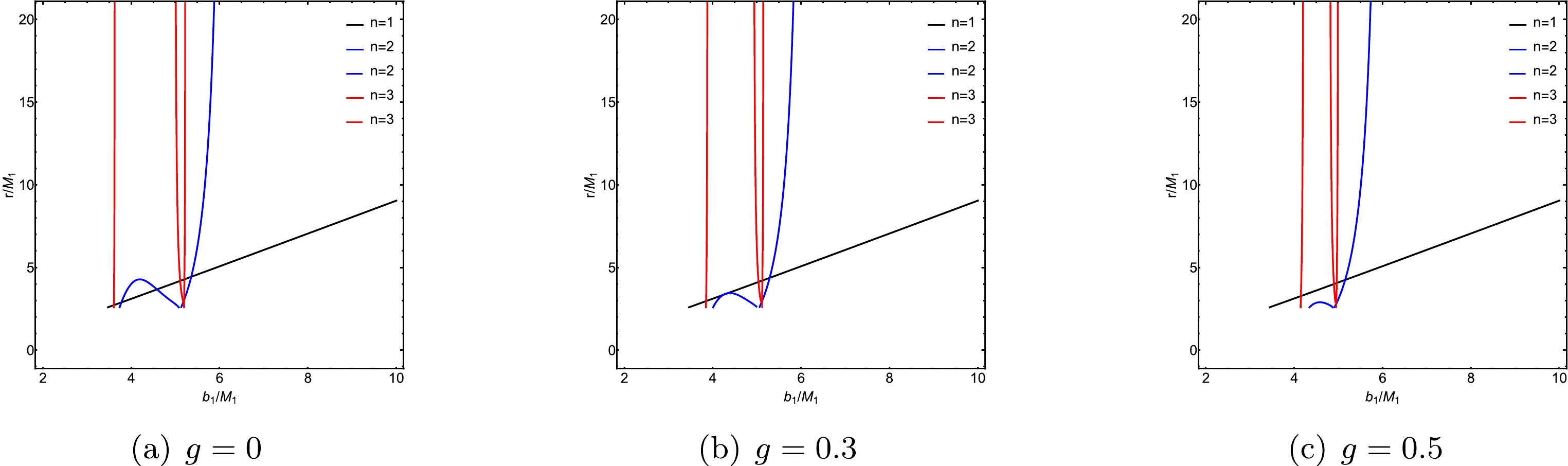

Figure 4.  (color online) Transfer functions for the ATSW with a Bardeen profile. We consider different magnetic charges g: $0,\,0.3,\,0.5$. The first transfer function is represented by the black lines, the second transfer function is represented by the blue lines, and the third transfer function is represented by the red lines. $M_1=1, M_2=1.2$, and $R=2.6$.

The transfer functions as the functions of impact parameter $b_1$ are shown in Fig. 4. The magnetic charge has three specific values g: $0,\,0.3,\,0.5$. We find that the first transfer functions (black lines) provide the "direct image" of the accretion disk, which owns a small demagnification factor. The second transfer functions (blue lines) produce a "lensing ring" with a large demagnification factor, which generates a reduced image for the back side of the accretion disk. The third transfer functions (red lines) exhibit the largest demagnification factor and represent a highly reduced image, which is known as the "photon ring" on the front side of the accretion disk.

Comparing the ATSW and BH cases, the ATSW has new second transfer functions ($n=2$), plotted by the blue dashed lines, which correspond to the "lensing band" [64]. There also exist new third transfer functions ($n=3$, the red dashed lines) near critical curves $Zb_{c_2}$ and $b_{c_1}$, which correspond to the "photon ring group" [65]. In addition, by comparing the demagnification factors of the new second transfer functions (see the dashed blue lines inFig. 4) for different magnetic charges g, one can find that as magnetic charge g increases, there is a higher demagnification factor of the new second transfer function.

In this section, we consider two emission models of the accretion disk to study the optical appearance of the ATSW. We believe that the image of the BH received by the observer is closely dependent on these emission models. One can use a Gaussian function to approximate the emission of the thin accretion disk. Given that $M_{1}=1$, the innermost stable circular orbit can be calculated, which is denoted as $r_{\rm isco}$. In emission model I, the radiation function is

where $r_{\rm isco}$ also represents the inner edge of the accretion disk, implying that no radiation is emitted within the region smaller than this inner edge. We plot the radiation function (22) in Fig. 5(a). In addition, we use emission model I to plot the observed intensity, density plot, and local density plot of the ATSW in the top panel of Fig. 6. For comparison, we also plot the optical appearance of the BH with the same mass parameter and radiation function in the bottom panel of Fig. 6. In Figs. 6(a) and 6(d), one can find that there exists a spatial separation between the direct emission, lensing band, and photon rings. For the ATSW case, it can be found that the direct emission with an initial intensity of $0.435$ appears near critical curve $b_1 \simeq 6.788M_{1}$, and then decreases, as shown in Fig. 6(a). In addition, the lensing band is confined from critical curve $b_1 \simeq 5.405M_{1}$ to the critical curve $b_1 \simeq 5.965M_{1}$. The photon rings appear near critical curves $b_1 \simeq 3.841 M_{1}$, $b_1 \simeq 4.948 M_{1}$, and $b_1 \simeq 5.131M_{1}$. Note that comparing the ATSW and BH cases, that is, Figs. 6(a) and 6(d), two additional photon rings appear near the critical curves $b_1 \simeq 3.841 M_{1}$, $b_1 \simeq 4.948 M_{1}$ in Fig. 6(a). From the density plot and the local density plot of the ATSW, one can find that the direct emission appears at the periphery of the black disk, while the narrow lensing band is confined within the black disk, which are shown in Figs. 6(b) and 6(c). In comparison to Figs. 6(e) and 6(f) (i.e., the BH case), we find that for the ATSW case, there are the two additional photon rings near the center of the black disk.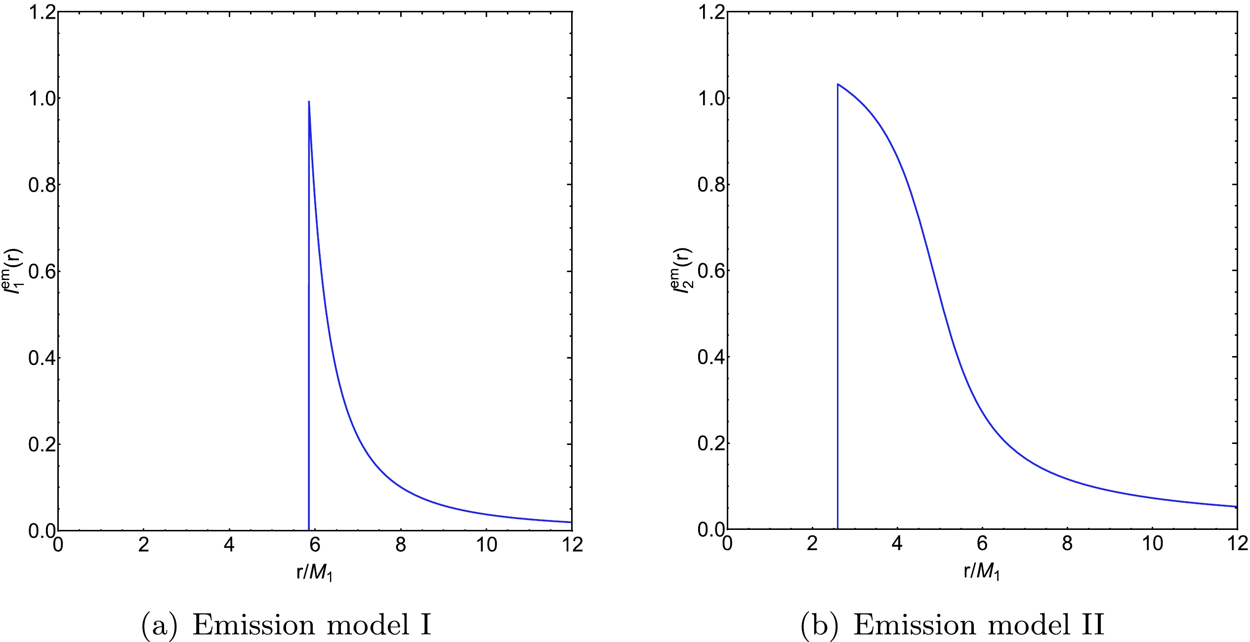

Figure 5.  (color online) Two emission models of the accretion disk.

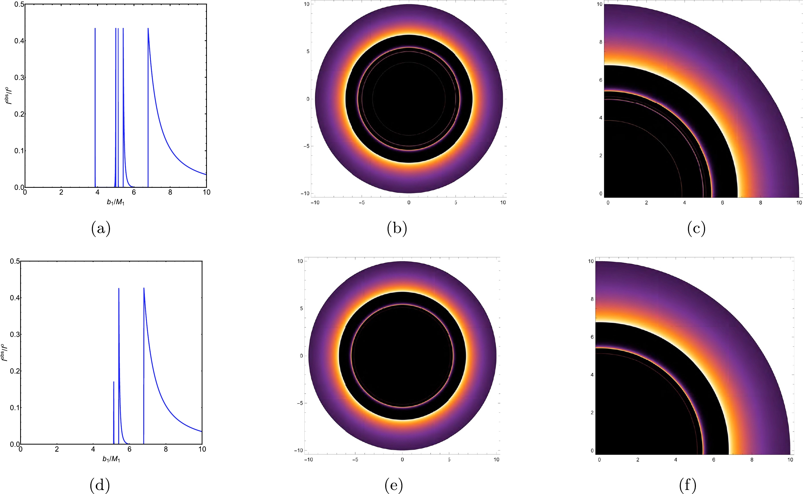
Figure 6.  (color online) In emission model I, observed intensities (left panel), density plots (middle panel), and local density plots (right panel) for the ATSW with a Bardeen profile (top panel) and Bardeen BH (bottom panel). We consider magnetic charge $g=0.3$, $M_1=1$, $M_2=1.2$, and $R=2.6$.

In emission model II, the radiation function is

in which $r_{h}$ denotes the event horizon radius. Hence, there is no radiation for the region smaller than the event horizon radius. We plot the radiation function (23) in Fig. 5(b). In comparison to emission model I, a more gradual decrease is observed for the radiation function of emission model II. Then, we use emission model II to plot the observed intensity, density plot, and local density plot of the ATSW in the bottom panel of Fig. 7. The optical appearance of the BH is also plotted in the bottom panel of Fig. 7. In Figs. 7(a) and 7(d), we find that there exists an overlap between the direct emission, lensing band, and photon rings in both the ATSW and BH cases. For the ATSW case, we find that the direct emission appears near critical curve $b_1 \simeq 2.822M_{1}$, as shown in Fig. 7(a). From Figs. 7(b) and 7(c), we find that there is a bright ring structure with multiple layers, as the photon rings are encompassed within the lensing band. We plot the optical appearance of the BH in the bottom panel of Fig. 7. From Figs. 6 and 7, it can be found that there is an extra lensing band between critical curves $Z b_{ c_{2}} \simeq$ 4.011 and $b_{ c_{1}} \simeq$ 5.051 for emission model II, which implies that in emission model II of the accretion disk for the ATSW, the new second transfer function could contribute to the observed intensity.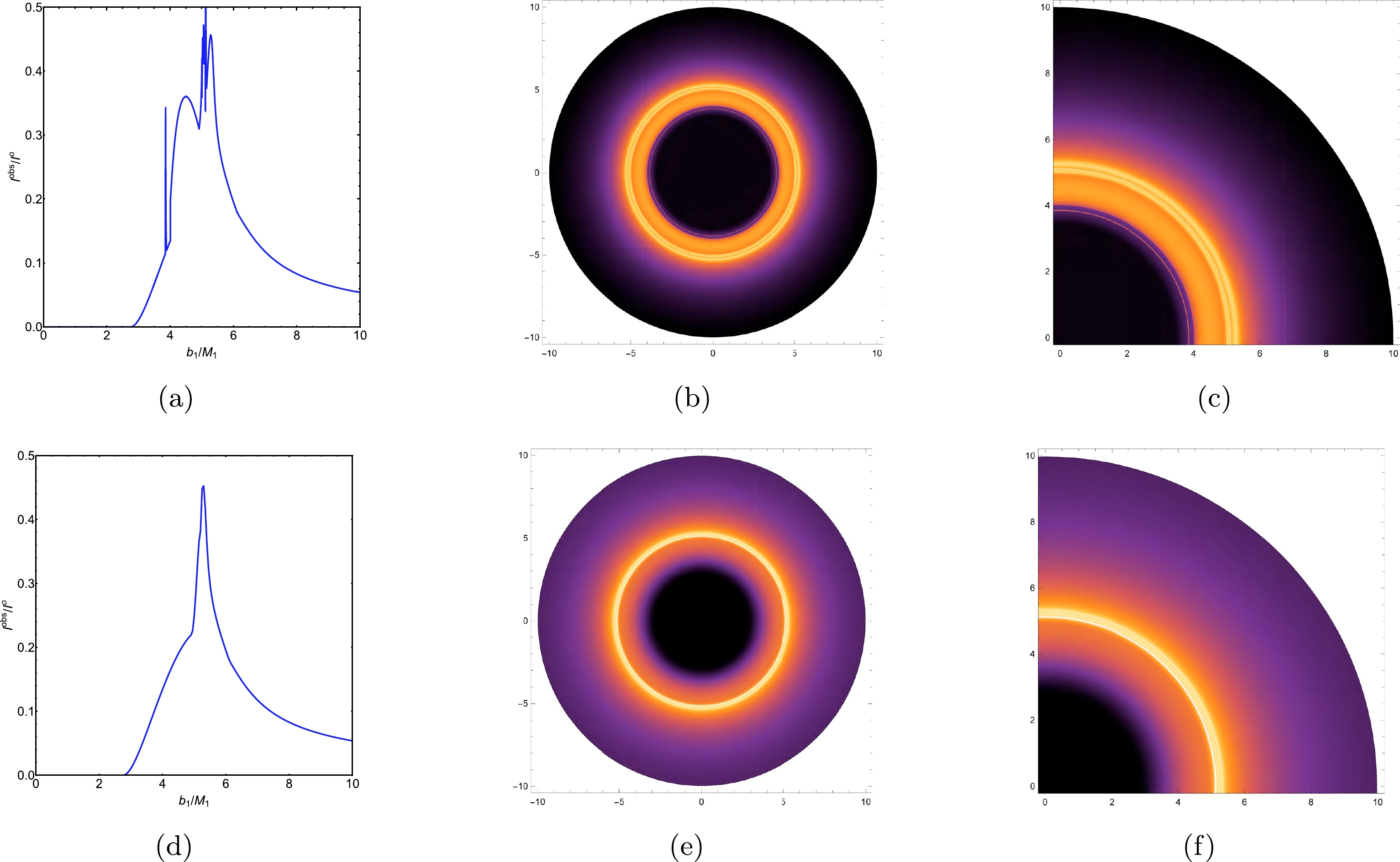

Figure 7.  (color online) In emission model II, observed intensities (left panel), density plots (middle panel), and local density plots (right panel) for the ATSW with a Bardeen profile (top panel) and Bardeen BH (bottom panel). We consider magnetic charge $g=0.3$, $M_1=1$, $M_2=1.2$, and $R=2.6$.

When $g=0$ (the Schwarzschild ATSW case), we also present the observed intensity, density plot, and local density plot in Fig. 8. Emission models I and II are employed in the top and bottom parts of Fig. 8, respectively. For the observational appearance of the Schwarzschild ATSW under emission model I, Fig. 8(a) shows that the direct emission appears near critical curve $b_1 \simeq 6.928M_{1}$. Two photon rings appear near critical curves $b_1 \simeq 5.056 M_{1}$ and $b_1 \simeq 5.210 M_{1}$, respectively. Moreover, the lensing band appears near critical curve $b_1 \simeq 5.472M_{1}$. For the case of emission model II, Fig. 8(d) shows that the direct emission appears near critical curve $b_1 \simeq 2.856M_{1}$. The results show that an increase in magnetic charge g leads to a decrease in the size of the light bands outside the shadow, which is consistent with the Bardeen BH case [86]. However, based on the observations from Fig. 8(a) and 8(d), it can be inferred that there exists an additional photon ring (corresponding to the newly introduced second transfer function) in close proximity to critical curve $b_1 \simeq 3.600 M_{1}$ under emission model I. Furthermore, there is an additional lensing band near critical curve $Z b_{ c_{2}} \simeq 3.742$ under emission model II. The results demonstrate that for the ATSW with a Bardeen profile, as magnetic charge g increases, there exists an increase in the size of the specific additional light bands. Hence, the trend of the influence of the change of magnetic charge g on the specific additional rings is opposite to the trend of the change of the related rings in the BH case.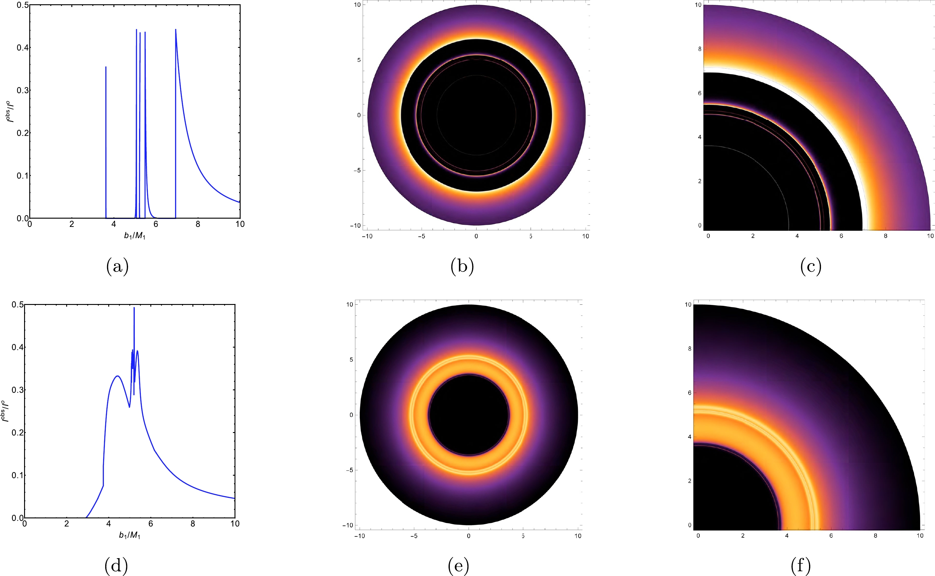

Figure 8.  (color online) Observed intensities (left panel), density plots (middle panel), and local density plots (right panel) of the Schwarzschild ATSW for emission model I (top panel) and emission model II (bottom panel). We consider $M_1=1$, $M_2=1.2$, and $R=2.6$.

To investigate the optical appearance of the ATSW with a Bardeen profile, we employ Visser's cut-and-paste method to construct an ATSW consisting of two spacetimes, ${\cal{M}}_{1}$ and ${\cal{M}}_{2}$. In this ATSW spacetime, one can assume that a static observer is situated in ${\cal{M}}_{1}$, and we present the calculated values for the related physical quantities, namely, photon sphere radius $r_{ph}$ and critical impact parameter $b_{c_{i}}$. The results demonstrate that as magnetic charge g increases, there is a decrease in both photon sphere radius $r_{ph}$ and critical impact parameter $b_{c_{i}}$. In other words, an increase in g leads to a contraction of the photon sphere towards the center. Then, we study the effective potentials of both the ATSW with a Bardeen profile and the Bardeen BH, as shown in Fig. 1. According to the impact parameter of the photon, its trajectory can be classified into three cases. If $b_1<Zb_{c_2}$, the photon in spacetime ${\cal{M}}_1$ will drop into spacetime ${\cal{M}}_2$ and then go to infinity in spacetime ${\cal{M}}_2$. If $Zb_{c_2}<b_1<b_{c_1}$, the photon in spacetime ${\cal{M}}_1$ will reach the turning point in spacetime ${\cal{M}}_2$ and then return to spacetime ${\cal{M}}_1$. If $b_1>b_{c_1}$, the photon in spacetime ${\cal{M}}_1$ will reach the turning point in spacetime ${\cal{M}}_1$ and then return to infinity in spacetime ${\cal{M}}_1$.

We study the trajectory and deflection angle of the photons, and then we plot their trajectories in Fig. 2. We find that as impact parameter $b_1$ decreases, the trajectory of the photon with impact parameter $Zb_{c_2}<b_1<b_{c_1}$ in spacetime ${\cal{M}}_{2}$ becomes longer. In addition, as magnetic parameter g increases, $b_{c_1}$ decreases, while $Zb_{c_2}$ increases. For the ATSW with a Bardeen profile, we also study the orbit number and number of intersections between the photon and accretion disk. The result shows that as magnetic charge g increases, the range of impact parameter $b_1$ decreases, which is consistent with the results presented in Table 1 and Fig. 2. The transfer functions of the ATSW are studied, and we find that there are new second and third transfer functions. The new second transfer function corresponds to the "lensing band", and the new third transfer function corresponds to the "photon ring group". In fact, when $Zb_{c_2}<b_1<b_{c_1}$, spacetime ${\cal{M}}_{2}$ can reflect photons back to spacetime ${\cal{M}}_{1}$, which leads to new transfer functions.

In two emission models of the accretion disk, we study the observational appearances of both the ATSW and BH. By comparing the ATSW and BH cases in emission model I, we find that there exist two extra photon rings near critical curves $b_1 \simeq 3.841 M_{1}$ and $b_1 \simeq 4.948 M_{1}$. In emission model II, an additional lensing band is observed between critical curve $Z b_{ c_{2}} \simeq 4.011$ and critical curve $b_{ c_{1}} \simeq 5.051$. By comparing the observational appearances of the Schwarzschild ATSW and the ATSW with a Bardeen profile, one can find that as magnetic charge g increases, there is an increase in the size of the specific additional light bands. Therefore, this may be a possible method to distinguish ATSWs from BHs by their observational appearances.