


 Abstract
 HTML
HTML Reference
 Related
 PDF
PDF


-
Quantum chromodynamics (QCD) describes the dynamics of quarks and gluons, underpinning nuclear physics from the hadronic mass spectrum to the phase transition of hadronic matter to quark-gluon plasma (QGP). Because of the nature of the strong interaction of QCD at a low energy scale, the perturbative method cannot be applied to explain low energy phenomena of nuclear physics. Fortunately, lattice QCD, which is based on first principles, can be employed to make precise predictions of hadronic quantities, especially phenomena that are difficult to explore in the laboratory, for example, the mass spectrum of baryons at different high temperatures.
In 1976, using the bag model, Jaffe predicted a flavour-singlet state (
$ uuddss $ ) with quantum number$I(J^P) =0(0^+)$ called H-dibaryon [1]. In contrast with the only known stable dibaryon (deuteron), whose binding energy is approximately$ 2.2\ {{\rm{MeV}}} $ , Jaffe predicted that the binding energy of the H-dibaryon is approximately$ 80\ {{\rm{MeV}}} $ below the$ \Lambda\Lambda $ threshold$ 2230\ {{\rm{MeV}}} $ , which means that the H-dibaryon is a deeply bound state.Unlike mesons and baryons, this exotic hadron may be relevant for the hypernuclei and the strange matter that could exist in the core of neutron stars. Moreover, it is a potential candidate for dark matter [2]. Thus, this prediction triggered an intense search for such a state, both experimentally [3–11] and theoretically [12–31].
The observation of double hypernuclei,
$ ^A_{\Lambda\Lambda}Z $ , is critical in connection with the existence of the H-dibaryon [3]. If the mass of the H-dibaryon,$ m_H $ , is much smaller than the mass of the double Λ hyperon,$ 2\,m_{\Lambda} $ , a double hypernuclei may decay into an H-dibaryon and a residual nucleus by strong interaction. In this case, the branching ratio for the decay of double hypernuclei through weak interaction is very small, which means that it cannot be observed in practice [3]. Therefore, the observation of the weak decay of double hypernuclei will set a limitation on the mass of the H-dibaryon,$m_H > 2\,m_{\Lambda} - B_{\Lambda\Lambda}$ , with$ B_{\Lambda\Lambda} $ being the binding energy of$ \Lambda\Lambda $ hyperons.Experiments [3–8, 11] investigated the nuclear capture of
$ \Xi^- $ at rest produced in the$ (K^-,K^+) $ reaction, analyzed the sequential weak decay of double hypernuclei, and measured the binding and interaction energies of$ \Lambda\Lambda $ [3, 5, 8, 11], or the cross section of the enhanced production of the$ \Lambda\Lambda $ pair [4, 6, 7]. The results do not confirm the existence of the H-dibaryon, but set a lower limit for its mass.Experiments [9, 10] were also conducted to search for the H-dibaryon or deeply bound singlet
$ uuddss $ sexaquark S (an explanation of S is provided in [2]) in the$ \Upsilon \rightarrow S\bar\Lambda\bar\Lambda $ decay. The results show no evidence for the existence of the H-dibaryon or S particle.Lattice QCD is used as a theoretical tool to investigate the H-dibaryon. Some quenched studies show that
$ m_H < 2\ m_{\Lambda} $ , suggesting that the H-dibaryon is a bound state [12–14]. However, other quenched studies show that the H-dibaryon is not a bound state [15–18].In addition to quenched studies, simulations with dynamical fermions have been carried out by NPLQCD, HALQCD, and other groups. The NPLQCD collaboration investigated baryon-baryon scattering and extracted the phase shift by employing Lüscher's method [32, 33] to distinguish scattering states from binding states [19–23, 34, 35]. They applied this methodology to determine whether the H-dibaryon exists by simulating with
$ N_f=2+1 $ dyamical fermions on anisotropic ensembles [20–22], and with$ N_f=3 $ dynamical fermions on isotropic ensembles [23].The HALQCD collaboration investigated the baryon-baryon interaction in terms of the baryon-baryon potential. They extracted the Nambu-Bethe-Salpeter wave-function by computing the four-point Green function on lattice, and then determined the baryon-baryon potential from the Nambu-Bethe-Salpeter wave-function. They applied this method to investigate the existence of the H-dibaryon on
$ N_f=3 $ [24–26] and$ N_f=2+1 $ [27–29] ensembles. The simulations on$ N_f=2+1 $ ensembles [27–29] conducted by HALQCD suggest that the H-dibaryon may be a$ \Lambda\Lambda $ resonance. Other results obtained by the two groups agreed on the presence of the H-dibaryon, despite disagreement on the binding energy [30].Ref. [30] reports on the simulation of ensembles of two dynamical quarks and one quenched strange quark. The authors applied Lüscher's method to determine the S-wave scattering phase shift with local and bilocal interpolators, and found a bound H-dibaryon for a pion mass of 960 MeV.
Ref. [31] reports on simulations based on O(a)-improved Wilson fermions at a SU(3) symmetric point with
$m_\pi=m_K\approx 420\;{ {\rm{MeV}}}$ . The results show that there exists a weakly bound H-dibaryon.In addition to the search for the H-dibaryon, lattice QCD calculations for three-flavored heavy dibaryons have been reported [36, 37]. These dibaryons are states with possible quark flavour combinations with at least one of them being charm (c) or bottom (b) quark.
Investigating the properties of hadrons at finite temperature, besides those at zero temperature, is among the central goals of lattice QCD simulations (see, for example, [38–44]). In the past decades, mesons at finite temperature have been studied extensively. This is not the case for baryons, which have been barely investigated at finite temperature on the lattice. There are a few lattice studies on baryonic screening and temporal masses [45–49]. Nevertheless, the behaviour of baryons in a hadronic medium is relevant to heavy-ion collisions. Therefore, there is a need for unambiguously understanding the property of baryons at finite temperature.
The present study on the H-dibaryon focused on the problem of its existence at zero temperature from different viewpoints. We conducted lattice QCD simulations to investigate the masses of the conjectured H-dibaryon and octet baryons at different temperatures. The change in the mass of the H-dibaryon with temperature is worth studying theoretically; moreover, the comparison of its mass with
$ m_\Lambda $ can provide some information on its existence.The paper is organized as follows. In Sec. II, we present details of the simulation technique, including the definition of correlation functions and interpolating operators. Sec. III introduces a method for extracting the spectral density from the correlation function designed in Ref. [50]. Our simulation results are presented in Sec. IV, followed by a discussion in Sec. V.
-
In our simulations, we computed the correlation functions of the H-dibaryon and Λ. We also calculated the correlation function of N, Σ, and Ξ. The generic form of a correlation function is
$ G(\vec{x},\tau) = < O(\vec{x},\tau)O^+(0)>, $

(1) and for the H-dibaryon interpolating operator, we chose the local operator. The starting point is the following operator notation for the different combinations of six quarks [30]:
$ \begin{aligned}[b] [abcdef] = \ & \epsilon_{ijk} \epsilon_{lmn} \Big( b^i C\gamma_5 P_+ c^j \Big) \\ & \times\Big( e^l C\gamma_5 P_+ f^m \Big) \Big( a^k C\gamma_5 P_+ d^n \Big) ({\vec{x}}, t)\,, \end{aligned} $

(2) where
$ a, b,\ldots,f $ denote generic quark flavors, and$P_+= (1+\gamma_0)/2$ projects the quark fields to positive parity. We chose the operator$O_{H}$ as the H-dibaryon interpolating operator which transforms under the singlet irreducible representation of flavor SU(3) [17, 51–53],$ O_{\bf{H}} = \frac{1}{48}\Big( [sudsud] - [udusds] - [dudsus] \Big), $

(3) and the H-dibaryon correlation function can be obtained from the formulae in Ref. [53].
For the baryon Λ interpolating operator, we chose the standard definition (see, for example, Refs. [54–56]),
$ \begin{aligned}[b] O_{\Lambda}(x) =\;& \frac{1}{\sqrt{6}} \epsilon_{abc} \left\{ 2 \left( u^T_a(x)\ C \gamma_5\ d_b(x) \right) s_c(x) \right. \\ & +\ \left( u^T_a(x)\ C \gamma_5\ s_b(x) \right) d_c(x) \\ & \left. -\ \left( d^T_a(x)\ C \gamma_5\ s_b(x) \right) u_c(x) \right\}\ , \end{aligned} $

(4) and for the correlation function of the baryon Λ, we also chose the standard definition (see, for example, Refs. [54–56]).
For the baryons N, Σ, and Ξ, we selected the corresponding standard definitions of the interpolating operator and correlator (see Refs. [54–56]).
After obtaining the correlation function, the mass can be obtained by fitting the exponential ansatz:
$ G(\tau) = A_+ {\rm e}^{-m_+\tau} + A_- {\rm e}^{-m_-(1/T-\tau)}, $

(5) where
$ m_{+} $ is the mass of the particle of interest, and τ takes values in the interval$ 0 \leq \tau<1/T $ on a lattice at finite temperature T.To obtain the ground state energy of the particle concerned, the best approach is to choose a large time extent lattice. However, at finite temperature, if the simulation is conducted on such a lattice, the lattice spacing must be small. Therefore, performing lattice simulations at finite temperature constitutes a dilemma presently. To obtain the ground state energy as accurately as possible on a relatively small time extent lattice, it is suitable for our procedure to incorporate an extrapolation method to obtain the ground state mass. We fit Eq. (5) to correlators in a series of time range
$ [\tau_1,\tau_2] $ , where$ \tau_2 $ is fixed to the whole time extent and$ \tau_1 $ is swept across several values:$\tau_1=1, 2, 3, ...$ Thus, we obtained a series of mass values corresponding to the suppression of different early Euclidean time slices. Subsequently, we plotted the mass values obtained in different time intervals$ [\tau_1,\tau_2] $ against$ 1/\tau_1 $ and fit a linear expression to those mass values. Finally, we extrapolated the linear expression to$ \tau_1 \to \infty $ . -
Hadron properties are encoded in spectral functions, which can provide important information on hadrons. Two approaches and their variants are usually adopted to reconstruct the spectral function. The first is the maximum entropy method and its variants [57–59]. The second is the Backus-Gilbert method and its variants [60–63] (reviews on the spectral function in lattice QCD can be found in Refs. [64, 65] and references therein). Recently, a new method based on the Backus-Gilbert method was presented in Ref. [50]. This method allows for choosing a smearing function at the beginning of the reconstruction procedure. To render this paper self-contained, we briefly present the method proposed in Ref. [50] in this section. In the following, the notations and symbols are almost the same as those used in Ref. [50].
The correlation function can be expressed as
$ G(\tau) = \int_0^\infty {\rm d} E\rho_L(E)b(\tau,E), $

(6) where
$ \rho_L(E) $ is the spectral function. We choose the basis function as$ b(\tau,E) = {\rm e}^{-\tau} + {\rm e}^{-(1/T-\tau)}, $

(7) and
$ \rho_L(E_\star) $ can be approximated by$ \bar{\rho}_L(E_\star) $ , where$ \bar{\rho}_L(E_\star) $ is evaluated by$ \bar{\rho}_L(E_\star) = \sum\limits_{\tau=0}^{\tau_{m}} g_\tau(E_\star) G(\tau+1), $

(8) once the coefficients
$ g_\tau(E_\star) $ are determined.The coefficients
$ g_\tau(E_\star) $ are determined by minimizing the linear combination$ W[\lambda,g] $ of the deterministic functional$ A[g] $ and error functional$ B[g] $ $ W[\lambda,g] = (1-\lambda) A[g] + \lambda \frac{B[g]}{G(0)^2}, $

(9) under the unit area constraint
$ \int_0^\infty {\rm d} E \bar\Delta_\sigma (E,E_\star) =1, $

(10) where
$ A[g] $ is defined as$ A[g] = \int_{E_0}^\infty {\rm d} E | \bar\Delta_\sigma (E,E_\star) - \Delta_\sigma (E,E_\star)|^2, $

(11) where
$ \bar\Delta_\sigma (E,E_\star) $ and$ \Delta_\sigma (E,E_\star) $ are the smearing and target smearing functions, respectively. These two functions are expressed as$ \bar\Delta_\sigma (E,E_\star) = \sum\limits_0^{\tau_m} g_\tau (\lambda, E_\star) b(\tau +1,E), $

(12) and
$ \Delta_\sigma (E,E_\star) = \frac{{\rm e}^{-\frac{(E-E_\star)^2}{2\sigma^2}}} {\int_0^\infty {\rm d} E {\rm e}^{-\frac{(E-E_\star)^2}{2\sigma^2}}} , $

(13) respectively.
$ B[g] $ is expressed as$ B[g]= g^T {{\rm{Cov}}} g, $

(14) where
$ { {\rm{Cov}}} $ is the covariance matrix of the correlation function$ G(\tau) $ . Further details are given in Ref. [50]. -
Before presenting the simulation results, we describe the computation details. The simulations were performed on
$ N_f=2+1 $ Generation2 (Gen2) FASTSUM ensembles [43]; the ensembles at the lowest temperatures were those provided by the HadSpec collaboration [66, 67]. The computation setup was the same as that used in Ref. [43]. We summarize the simulation details in Tables 1, 2, and 3 from Ref. [43].Gauge coupling (fixed-scale approach) $ \beta = 1.5 $ 

tree-level coefficients $ c_0=5/3,\,c_1=-1/12 $ 

bare gauge, fermion anisotropy $ \gamma_g = 4.3 $ ,

$ \gamma_f = 3.399 $ 

ratio of bare anisotropies $ \nu = \gamma_g / \gamma_f = 1.265 $ 

spatial tadpole (without, with smeared links) $ u_s = 0.733566 $ ,

$ \tilde{u}_s = 0.92674 $ 

temporal tadpole (without, with smeared links) $ u_\tau = 1 $ ,

$ \tilde u_\tau = 1 $ 

spatial, temporal clover coefficient $ c_s = 1.5893 $ ,

$ c_\tau = 0.90278 $ 

stout smearing for spatial links $ \rho = 0.14 $ , isotropic, 2 steps

bare light quark mass for Gen2 $ \hat m_{0, {\rm{light}}} = -0.0840 $ 

bare strange quark mass $ \hat m_{0, {\rm{strange}}} = -0.0743 $ 

light quark hopping parameter for Gen2 $ \kappa_{{\rm{light}}} = 0.2780 $ 

strange quark hopping parameter $ \kappa_{{\rm{strange}}} = 0.2765 $ 

Table 1. Parameters in the lattice action. This table is recompiled from Ref. [43].
$ a_\tau $ /fm

0.0350(2) $ a_\tau^{-1} $ /GeV

5.63(4) $ \xi=a_s/a_\tau $ 

3.444(6) $ a_s $ /fm

0.1205(8) $ N_s $ 

24 $ m_\pi $ /MeV

384(4) $ m_\pi L $ 

5.63 Table 2. Parameters such as lattice spacing and pion mass from Ref. [43] for Generation 2 ensemble.
$ N_s $ 

$ N_\tau $ 

$T /{\rm MeV}$ 

$ T/T_c $ 

$ N_{{\rm{cfg}}} $ 

$ a_\tau m_N $ 

$ a_\tau m_\Sigma $ 

$ a_\tau m_\Xi $ 

$ a_\tau m_{\Lambda} $ 

$ a_\tau m_H $ 

24 128 44 0.24 304 0.2133(24)(6) 0.2349(21)(5) 0.2459(18)(5) 0.2299(23)(6) 0.457(27)(5) 32 48 117 0.63 601 0.208(2)(3) 0.231(1)(2) 0.243(1)(2) 0.226(2)(3) 0.448(17)(4) 24 40 141 0.76 502 0.203(2)(5) 0.228(2)(4) 0.239(2)(4) 0.221(2)(4) 0.437(14)(9) 24 36 156 0.84 501 0.196(2)(6) 0.221(2)(5) 0.231(2)(5) 0.214(2)(5) 0.42(1)(2) 24 32 176 0.95 1000 0.181(2)(9) 0.204(2)(8) 0.215(2)(7) 0.199(2)(8) 0.393(7)(21) 24 28 201 1.09 1001 0.179(2)(12) 0.191(2)(12) 0.201(2)(11) 0.190(2)(11) 0.38(1)(2) 24 24 235 1.27 1001 0.172(3)(15) 0.179(3)(15) 0.191(3)(14) 0.182(3)(14) 0.36(1)(3) 24 20 281 1.52 1000 0.159(4)(18) 0.164(4)(18) 0.176(4)(17) 0.169(4)(17) 0.33(1)(4) 24 16 352 1.90 1000 0.154(6)(24) 0.158(6)(24) 0.171(6)(23) 0.164(6)(23) 0.31(2)(4) Table 3. Spatial and temporal extent, temperature in MeV, number of configurations, and masses of N, Σ, Ξ, Λ, and H-dibaryon. Masses of baryons and H-dibaryon are obtained by the extrapolation method. Estimates of statistical and systematic errors are contained in the first and second brackets, respectively. The errors of the fitting parameters of linear extrapolation are the systematic errors of the masses. The ensembles at the lowest temperatures are those provided by HadSpec [66, 67] (Gen2).
The ensembles were generated with a Symanzik-improved gauge action and a tadpole-improved clover fermion action with stout-smeared links. The details of the action are given in Ref. [43]. The parameters in the lattice action are recompiled in Table 1. The
$ N_f=2+1 $ Gen2 ensembles correspond to a physical strange quark mass and a bare light quark mass of$ a_\tau m_l=-0.0840 $ , yielding a pion mass of$ m_\pi=384(4) $ MeV (see Table 2).The ensemble details are listed in Table 3, which is recompiled from Ref. [43] with a slight difference on the ensemble
$ N_s^3\times N_\tau = 32^3\times 48 $ . The corresponding physical parameters, such as lattice spacing and pion mass, are listed in Table 2.The quark propagators were computed using the deflation-accelerated algorithm [68, 69]. When computing the propagator, the spatial links were stout smeared [70] with two steps of smearing, using the weight
$ \rho = 0.14 $ . For the sources and sinks, we used Gaussian smearing [71],$ \eta' = C\left(1+\kappa H\right)^n\eta, $

(15) where H is the spatial hopping part of the Dirac operator, and C is an appropriate normalization factor [49].
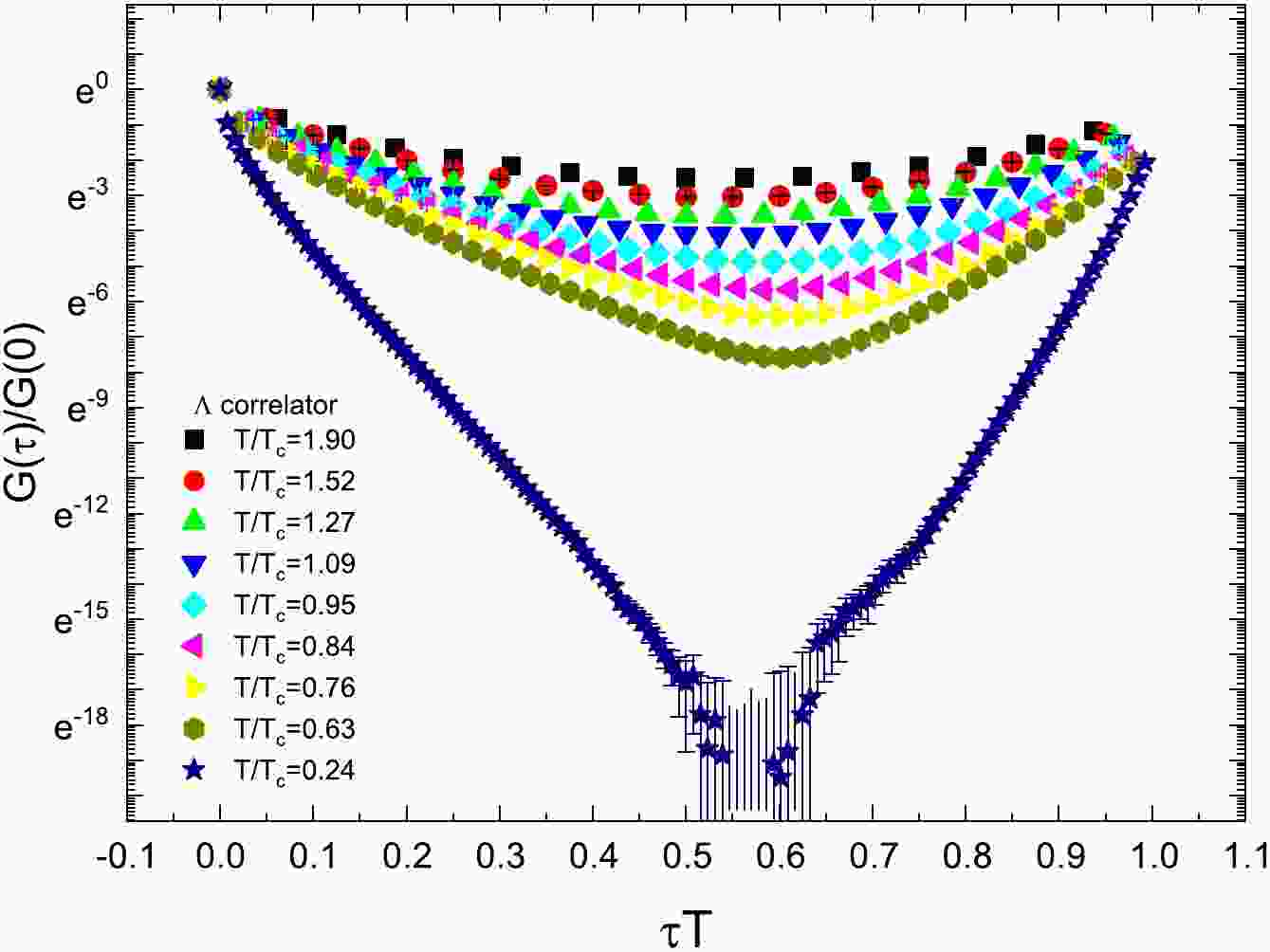
The correlators of the Λ and H-dibaryon are presented in Figs. 1 and 2, respectively. For the correlators of the Λ and H-dibaryon, we found a similar behavior to that displayed in Fig. 1 in Ref. [49] for N. For the correlator of Λ on large
$ N_\tau $ and relatively small$ N_s $ lattice, especially the$ 24^3\times 128 $ lattice, some correlator data points take negative values. These points are not depicted in the plot because the vertical axis is rescaled logarithmically. At some points, the error bar looks strange. It is because, at these points, the errors reach the magnitude of the correlator value, and the vertical axis is rescaled. For the plot of the H-dibaryon correlator, the same observation can be made.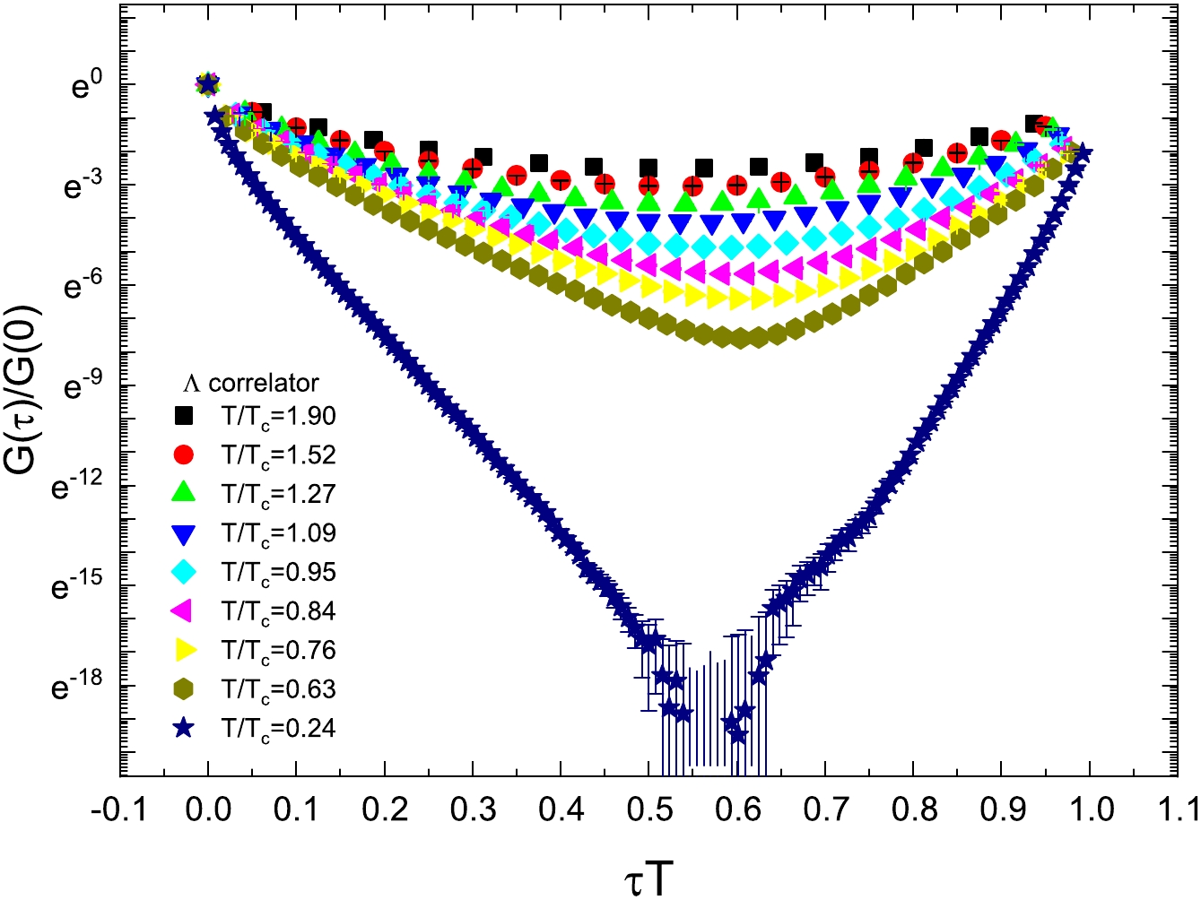
Figure 1. (color online) Euclidean correlator
$ G(\tau)/G(0) $ of Λ as a function of$ \tau T $ at different temperatures. At the lowest temperature$ T/T_c =0.24 $ , the correlators at some points are not displayed because they take negative values.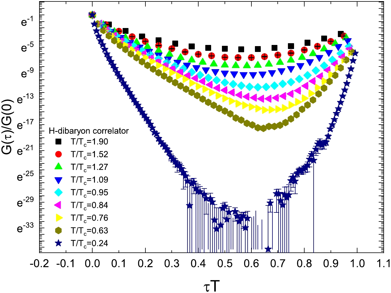
Figure 2. (color online) Euclidean correlator
$ G(\tau)/G(0) $ of H-dibaryon as a function of$ \tau T $ at different temperatures. At the lowest temperature$ T/T_c =0.24 $ , the correlators at some points are not displayed because they take negative values.We used the extrapolation method to extract the ground state masses for N, Ξ, Σ, Λ, and H-dibaryon. We first fit Eq. (5) to the correlator by suppressing different early time slices to obtain a series of mass values. We present the results of nucleon and H-dibaryon on lattice
$ N_\tau=128 $ in Fig. 3. After obtaining a series of mass values with different early time slices suppressed, we extrapolated the mass values linearly according to the scenario described in the last paragraph in Sec. II. We present the results of linear extrapolation for the nucleon and H-dibaryon on lattice$ N_\tau=128 $ in Fig. 4. In the extrapolation procedure, we used one portion of the data presented in Fig. 3.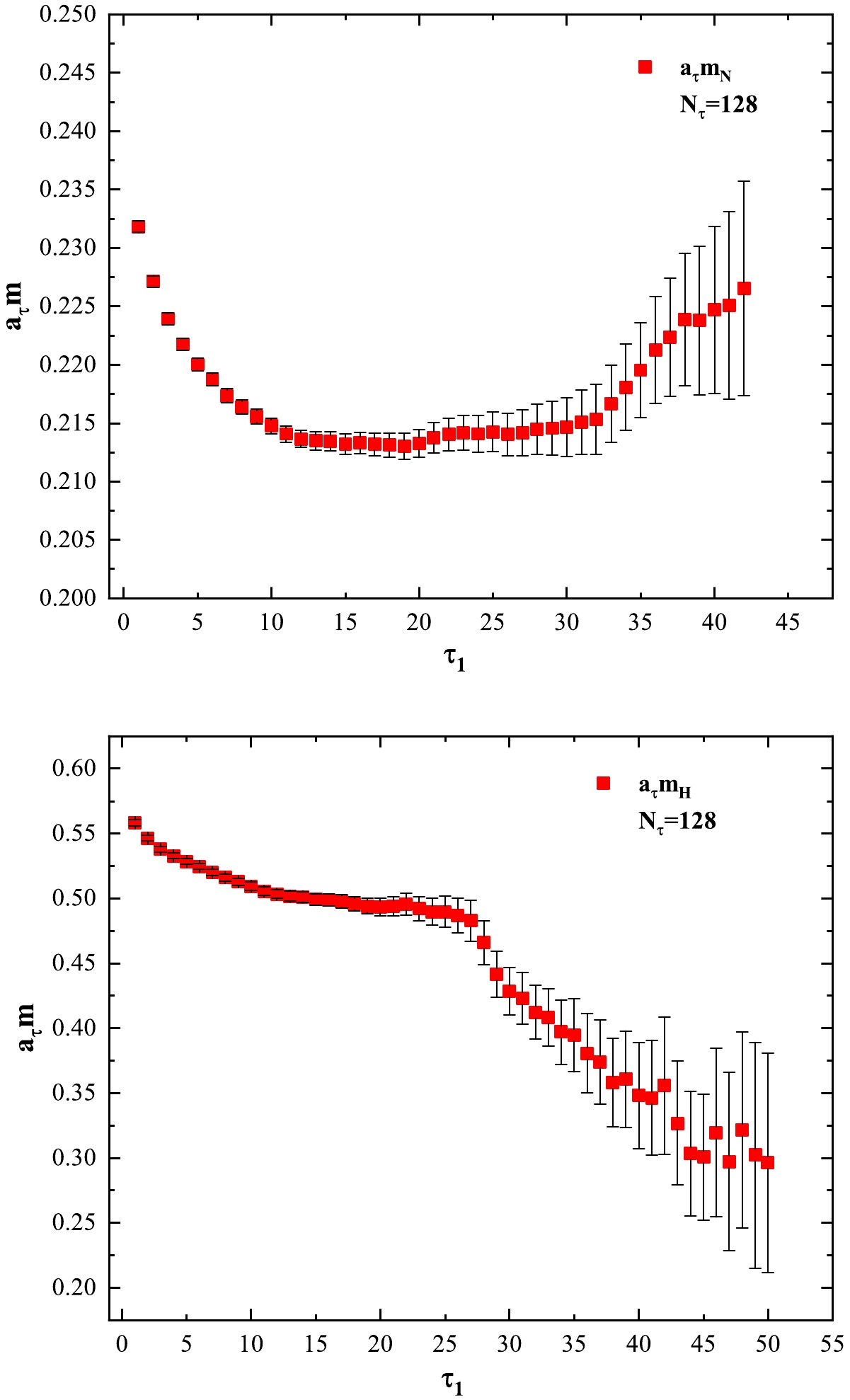
Figure 3. (color online) Mass values of nucleon and H-dibaryon obtained by fitting Eq. (5) to correlators on
$ N_\tau=128 $ ensembles. The mass values are the fitting parameter$ m_+ $ in Eq. (5) extracted by the fitting procedure in different intervals$ [\tau_1, \tau_2] $ . The horizontal axis label$ \tau_1 $ represents different number of time slices suppressed corresponding to the lower bound of the interval$ [\tau_1, \tau_2] $ .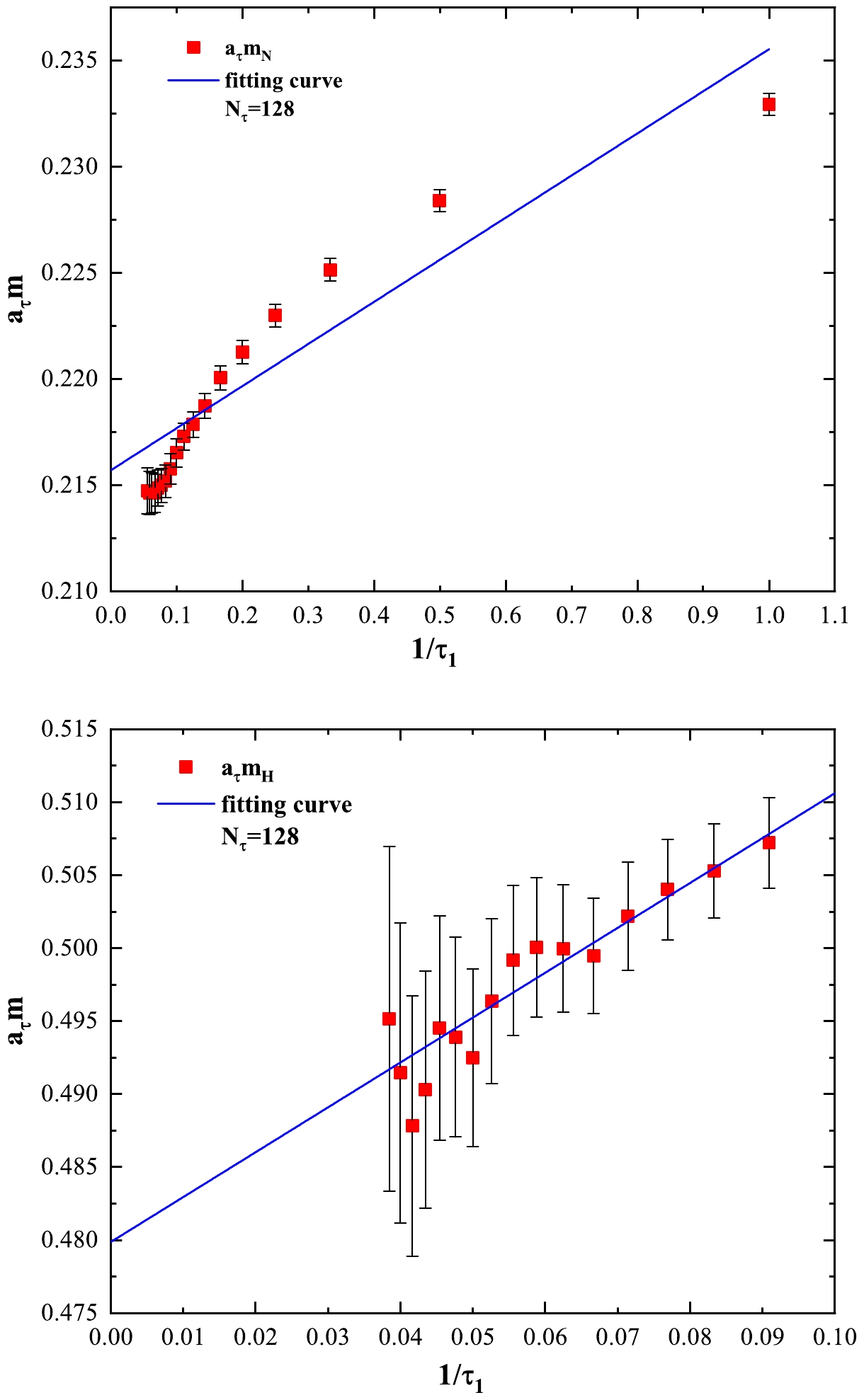
Figure 4. (color online) Linear extrapolation of mass values for nucleon and H-dibaryon on
$ N_\tau=128 $ ensembles. The horizontal axis represents inverse values of time slices suppressed.The results are listed in Table 3. Note that the masses decrease when the temperature increases. We compare our results of N and Λ below
$ T_c $ with those in Refs. [45, 49]. The results are consistent within errors.We also calculated the spectral density
$ \bar\rho_L(E_\star) $ of the correlation function of N, Σ, Ξ, Λ, and H-dibaryon using a public computer program [72].We present the spectral density for
$ \sigma = $ 0.02, 0.04, 0.06, and 0.08 and N, Ξ, and H-dibaryon at three temperatures in Fig. 5. The upper panel in Fig. 5 for N at$ T/T_c = 0.24 $ indicates that too large σ values may skip the peak structure of spectral density. Note from the upper panel in Fig. 5 that the spectral density distribution obtained for$ \sigma = 0.08 $ has only one position where$ \bar\rho_L(E_\star) $ takes a local maximum value. This position is approximately at$ E_\star =0.37 $ . At$ T/T_c =0.24 $ , the time extent$ N_\tau=128 $ is large enough to extract the ground state energy.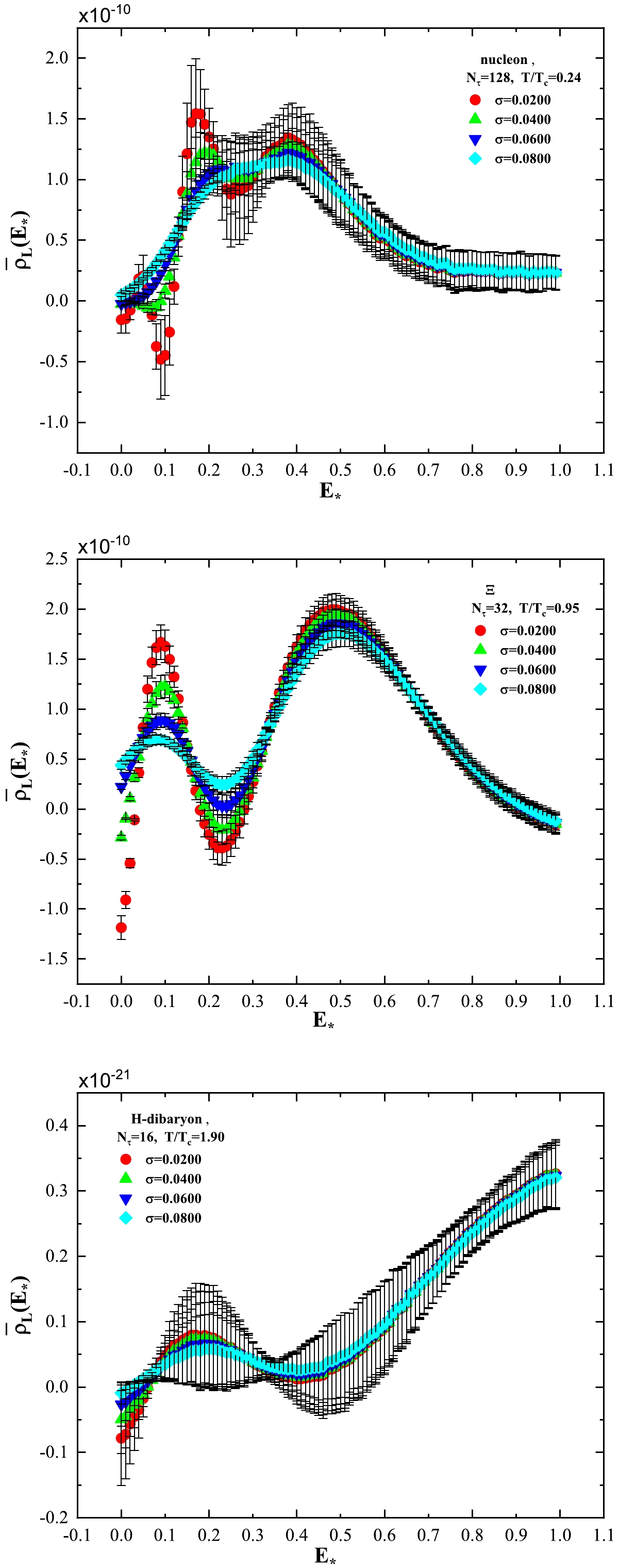
Figure 5. (color online) Spectral density computed with different values of the parameter σ for the target smearing function
$ \Delta_\sigma (E,E_\star) $ for H-dibaryon, Ξ, and N at different temperatures.However, even if we do not suppress any early Euclidean time slices in the fitting procedure based on Eq. (5), we cannot obtain a mass value
$ a_\tau m_N $ larger than$ 0.30 $ . The largest value of$ a_\tau m_N $ that we obtained by suppressing different numbers of early time slices was approximately 0.25, which is smaller than 0.30, as can be clearly seen from Fig. 3. The mass value of 0.30 is somewhat an arbitrary value between the two peak positions of 0.17 and 0.38 for the spectral density presented in Table 4. Thus, we conclude that setting a large σ value may lead to missing some peak structures. By contrast, the spectral density$ \bar\rho_L(E_\star) $ obtained for$ \sigma = 0.02 $ in the upper panel of Fig. 5 has a peak position at$ E_\star \approx 0.05 $ with a small peak value. This peak structure may be due to lattice artifacts.$ N_\tau $ 

$ E_\star $ 

$ E_\star $ 

$ E_\star $ 

N 128 0.05 0.17 0.38 48 0.06 0.35 – 40 0.09 0.42 – 36 0.10 0.52 – 32 0.11 0.56 – 28 0.18 0.57 – 24 0.26 – – 20 0.24 – – 16 0.43 – – Table 4. For different
$ N_\tau $ lattices, peak position$ E_\star $ of the spectral density for N.$ N_\tau $ 

$ E_\star $ 

$ E_\star $ 

$ E_\star $ 

Σ 128 0.05 0.17 0.37 48 0.06 0.35 – 40 0.08 0.41 – 36 0.09 0.49 – 32 0.11 0.56 – 28 0.17 0.57 – 24 0.20 – – 20 0.22 – – 16 0.39 – – Table 5. For different
$ N_\tau $ lattices, peak position$ E_\star $ of the spectral density for Σ.$ N_\tau $ 

$ E_\star $ 

$ E_\star $ 

Ξ 128 0.05 0.33 48 0.06 0.34 40 0.08 0.41 36 0.09 0.48 32 0.10 0.55 28 0.13 0.63 24 0.17 0.71 20 0.20 – 16 0.32 – Table 6. For different
$ N_\tau $ lattices, peak position$ E_\star $ of the spectral density for Ξ.$ N_\tau $ 

$ E_\star $ 

$ E_\star $ 

$ E_\star $ 

Λ 128 0.05 0.18 0.38 48 0.06 0.35 – 40 0.08 0.42 – 36 0.09 0.49 – 32 0.11 0.56 – 28 0.14 0.61 – 24 0.18 0.64 – 20 0.22 – – 16 0.35 – – Table 7. For different
$ N_\tau $ lattices, peak position$ E_\star $ of the spectral density for Λ.$ N_\tau $ 

$ E_\star $ 

$ E_\star $ 

$ E_\star $ 

$ E_\star $ 

H-dibaryon 128 0.10 0.19 0.35 0.69 48 0.05 0.24 0.64 – 40 0.06 0.32 0.78 – 36 0.07 0.35 – – 32 0.08 0.45 – – 28 0.10 0.52 – – 24 0.11 – – – 20 0.14 – – – 16 0.17 – – – Table 8. For different
$ N_\tau $ lattices, peak position$ E_\star $ of the spectral density for H-dibaryon.The middle panel in Fig. 5 for Ξ at
$ T/T_c = 0.95 $ shows that smaller σ values can lead to a more pronounced peak structure of the spectral density in small$ E_\star $ regions. The lower panel for the H-dibaryon at$ T/T_c = 1.90 $ suggests that setting different σ values has little effect on the computation of spectral density at high temperature. Therefore, we only present the spectral density results computed for$ \sigma =0.020 $ in the following.The spectral density
$ \bar\rho_L(E_\star) $ of Ξ, Λ, and H-dibaryon is presented in Figs. 6, 7, and 8, respectively. The spectral density$ \bar\rho_L(E_\star) $ of N and Σ has a similar behaviour to that of Λ. Note from Figs. 6, 7, and 8 that the spectral density$ \bar\rho_L(E_\star) $ of Ξ and Λ has a similar behaviour, while$ \bar\rho_L(E_\star) $ of the H-dibaryon is slightly different. All the peak positions of$ \bar\rho_L(E_\star) $ are provided in Tables 4−8.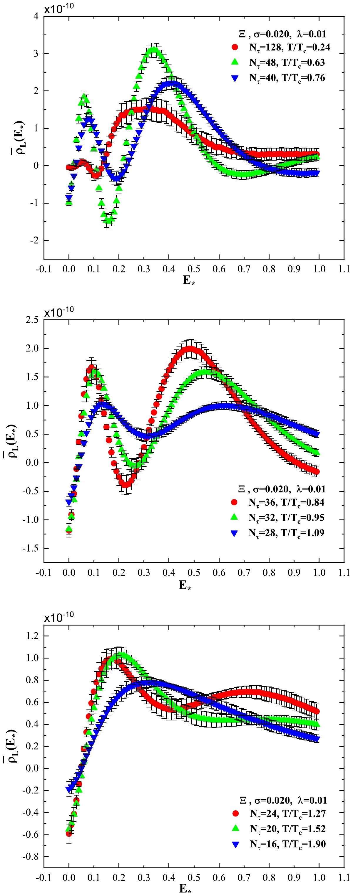
Figure 6. (color online) Spectral density of Ξ at different temperatures.
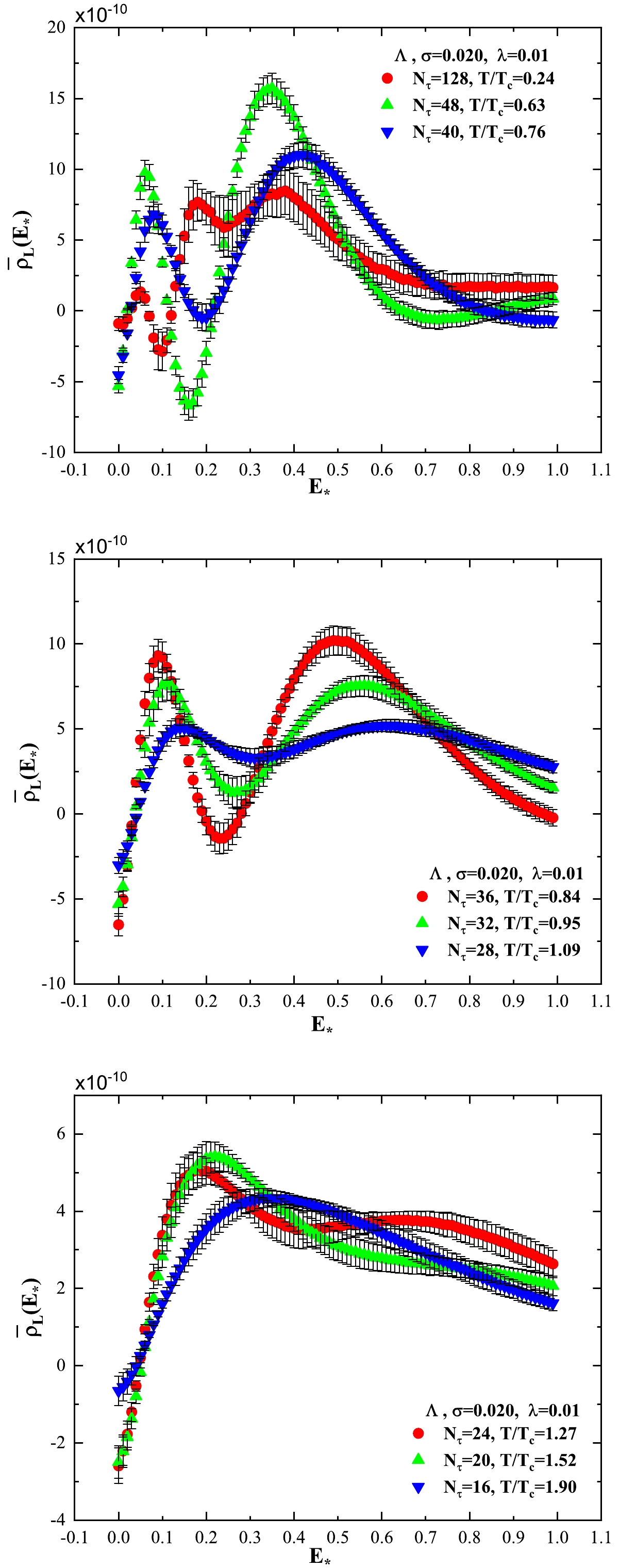
Figure 7. (color online) Spectral density of Λ at different temperatures.
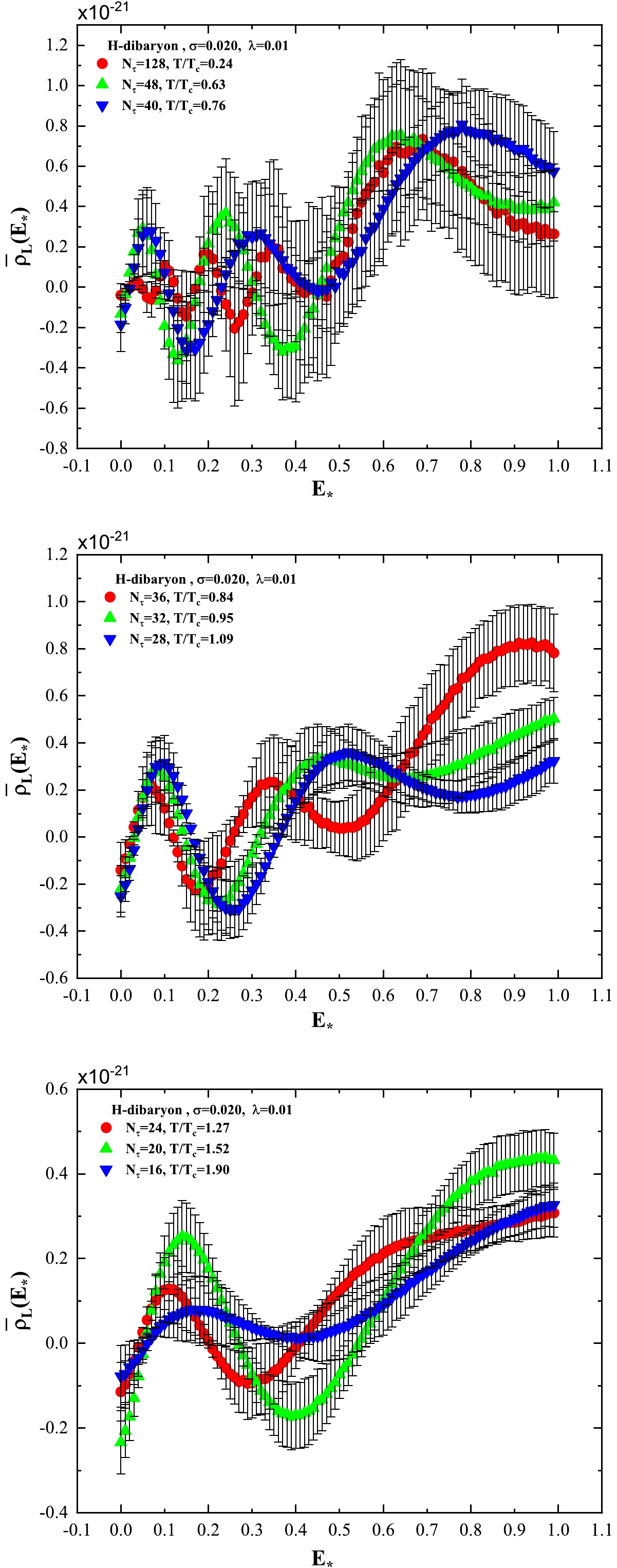
Figure 8. (color online) Spectral density of H-dibaryon at different temperatures.
Note from Figs. 6, 7, and 8 that, at the lowest temperature
$ T/T_c = 0.24 $ , the spectral density for Ξ, Λ, and H-dibaryon has a rich peak structure. Despite the two peaks approximately located between$ E_\star=0.20 $ and$ E_\star=0.40 $ , the spectral density$ \bar\rho_L(E_\star) $ of Ξ and Λ in the range of$ E_\star $ from$ 0.20 $ to$ 0.40 $ are approximately the same. The mass values$ a_\tau m_\Xi = 0.2459 $ and$ a_\tau m_\Lambda = 0.2299 $ obtained by the extrapolation method lie in that range of$ E_\star $ .However,
$ a_\tau m_H = 0.44 $ at$ T/T_c = 0.24 $ for the H-dibaryon is in the neighborhood of the peak position$ E_\star = 0.35 $ , where the$ \bar\rho_L(E_\star) $ value is not very large. Note that$ a_\tau m_H = 0.44 $ at$ T/T_c = 0.24 $ is obtained by suppressing more early Euclidean time slices. The upper panel of Fig. 8 shows that more high frequency components of the spectral density should be suppressed in the extrapolation procedure.When temperature increases, the multi-peak structure of the spectral density distribution turns into a two-peak structure for Ξ and Λ, and at high temperatures, i.e.,
$ T/T_c = $ 1.27, 1.52, and 1.90, the spectral density distribution presents one peak.At intermediate temperatures, the spectral density
$ \bar\rho_L(E_\star) $ exhibits a two-peak structure. If we take the smaller values of$ E_\star $ at peak positions as the ground state energies of the corresponding particle, then these mass values obtained by the peak position of$ \bar\rho_L(E_\star) $ are smaller than those mass values obtained in Refs. [49] and [45]. The mass values of$ a_\tau m_\Xi $ ,$ a_\tau m_\Lambda $ , and$ a_\tau m_H $ presented in Table 3 are not consistent with the peak positions of the corresponding spectral density. Note that the mass values obtained by the extrapolation method are affected by the two-peak structure of the spectral density.At high temperatures, i.e.,
$ T/T_c = $ 1.27, 1.52, and 1.90, the spectral density distribution for N exhibits one peak structure, and the peak position shifts towards large values with increasing temperature. Note that the peak broadens and becomes smooth. It means that in the mass spectrum structure of the nucleon, there is no δ function structure contributing to the correlation function, as shown in Fig. 9 for N. A similar behaviour can be found for Σ, Ξ, and Λ. The smooth distribution of the spectral density implies that a one-particle state does not exist at high temperature.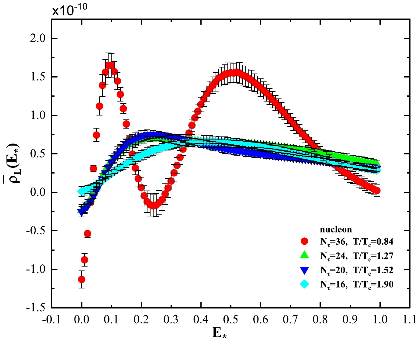
Figure 9. (color online) Spectral density distribution of N at different temperatures:
$ T/T_c = $ 0.84, 1.27, 1.52, and 1.90. At$T/T_c = 0.84,~ N_\tau = 36$ , the spectral density of N exhibits two peaks. At$ T/T_c = $ 1.27, 1.52, and 1.90, the spectral density distribution becomes approximately smooth.This is not the case for the H-dibaryon. Its spectral density distribution at
$ T/T_c = 0 $ , 1.27, 1.52, and 1.9 is presented in Fig. 10. Note that, at$ T/T_c = $ 1.27 and 1.52, the spectral density distribution still exhibits a one peak structure; at$ T/T_c = 1.90 $ , the spectral density distribution broadens and becomes smooth. This observation may imply that, at temperatures$ T/T_c = $ 1.27 and 1.52, the H-dibaryon still exhibits a one-particle state.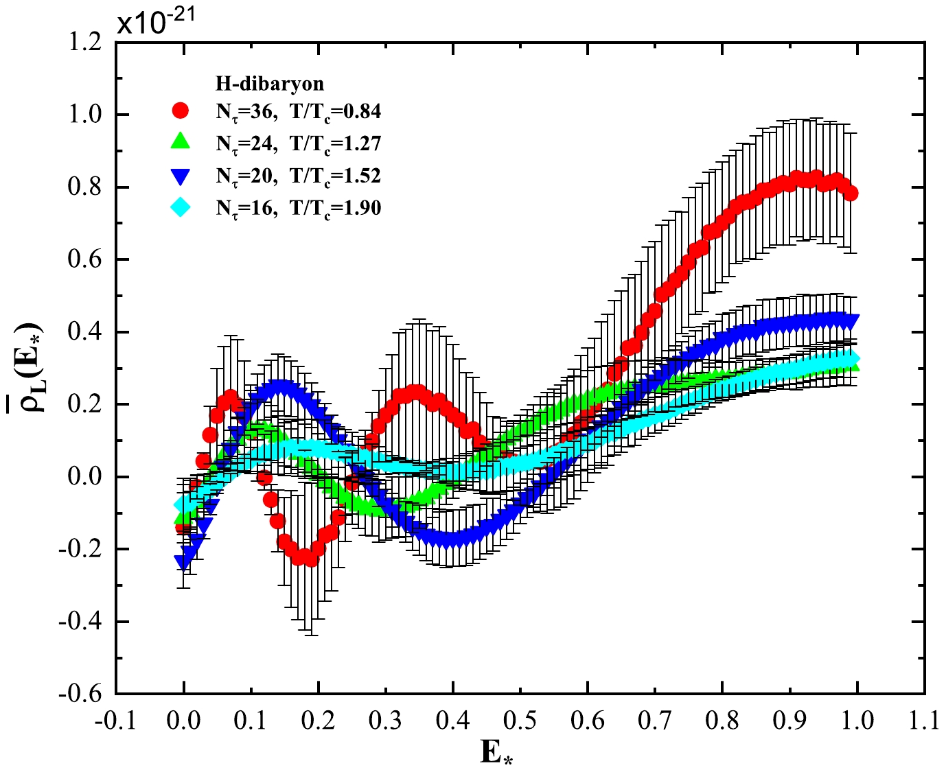
Figure 10. (color online) Spectral density distribution of the H-dibaryon at different temperatures:
$T/T_c = 0.84, 1.27, 1.52, $ $ {\rm and}\;1.90$ . At$ T/T_c = 0.84, N_\tau = 36 $ , the spectral density of the H-dibaryon exhibits two peaks. At$ T/T_c = 1.27, 1.52 $ , the spectral density distribution has one peak. At$ T/T_c = 1.90 $ , the spectral density distribution becomes approximately smooth. -
We conducted simulations aiming to determine the masses of the conjectured H-dibaryon using the
$ 2+1 $ flavor QCD with clover fermion at nine different temperatures. We also calculated the masses of N, Σ, Ξ, and Λ. The results are presented in Table 3. The spectral density distribution of the correlation function of these particles was computed to understand the mass spectrum obtained by the extrapolation method.In our simulations, the change in temperature was represented by the change in
$ T/T_c $ , where$ T_c $ is the pseudocritical temperature determined via the renormalized Polyakov loop and estimated to be$T_c = 185(4)~ {\rm MeV}$ [43, 73].We compared two scenarios to obtain the ground state mass as accurately as possible. One is based on suppressing more early Euclidean time slices in the fitting procedure with Eq. (5). The second is based on the extrapolation method. We extrapolated some fitting results obtained for different suppressions of Euclidean time slices and time approaching infinity. The results from both methods are consistent within errors. We only present the results from the extrapolation method in Table 3. Among the series of mass values obtained by different early time suppressions, it is difficult to choose which mass value is the proper one. However, the extrapolation method can alleviate this difficulty to some extent.
The analysis of spectral density can provide insights on mass spectrum. However, in our simulations, we found that the mass values obtained by the extrapolation method are not consistent with the peak position of the spectral density in some cases, especially at high temperature. In this case, we consider that the results provided by the extrapolation method are more reliable. The peak positions for the nucleon in Table 4 can be selected as an example to give an explanation. The smaller values of the peak positions increase with temperature. However, the mass values of the corresponding particle are supposed to decrease with increasing temperature.
At the lowest temperature
$ T/T_c = 0.24 $ , the spectral density distribution has a rich peak structure. The mass spectrum of particles approximately reflects the peak position of the spectral density distribution.At intermediate temperatures, the spectral density distribution exhibits a two-peak structure. The peak structure at the smaller
$ E_\star $ gradually becomes smooth when σ increases. Considering the quark mass corresponding to$ m_\pi=384(4){{\rm{MeV}}} $ , if we take the smaller$ E_\star $ at the peak position as the ground state energy, the resulting mass value is too small. Thus, we conclude that the mass values obtained by using the extrapolation method are affected by the two states.At high temperature, we obtained the mass values for N, Σ, Ξ, and Λ, listed in Table 3, using the extrapolation method. Note that the spectral density distribution appears to become smooth, which implies that a one-particle state does not exist.
The H-dibaryon is a multi-baryon state. Note from the spectral density distribution that, at the lowest temperature
$ T/T_c = 0.24 $ , the multi-state structure manifests. When temperature increases, the number of peaks decreases until reaching$ T/T_c = 1.90 $ , at which the spectral density distribution becomes approximately smooth. This means that it is likely that the H-dibaryon survives beyond$ T_c $ until it melts down at$ T/T_c = 1.90 $ . Considering that the H-dibaryon is a multi-baryon state, this conclusion calls for further investigation.It is appropriate to consider the lowest temperature ensembles
$ N_\tau=128 $ to be those of the zero temperature given that$ N_\tau>\xi N_s $ [43]. Using the mass values of the H-dibaryon and Λ in Table 3 at$ N_\tau=128, ~T/T_c = 0.24 $ , an estimation of$ \Delta m = m_H - 2m_\Lambda $ can be made,$ \Delta m = m_H - 2m_\Lambda = -0.0026(11) $ , which is converted into physical units to be$ \Delta m = m_H - 2m_\Lambda = -14.6(6.2) $ MeV. Refs. [23, 25, 26, 30, 31, 35] reported the presence of a binding state of the H-dibaryon, despite disagreement on the binding energy values. Refs. [23, 35] reported a binding energy of$ 16.6 \pm 2.1 $ MeV at$ m_\pi= 389 $ MeV, and$ 74.6 \pm 4.7 $ MeV at$ m_\pi= 800 $ MeV. Ref. [25] reported a binding energy for the H-dibaryon of$ 30-40 $ MeV for a pion mass of$ 673-1015 $ MeV. Ref. [26] reported similar results. Ref. [30] published a binding energy of$ 19 \pm 10 $ MeV for the H-dibaryon at$ m_\pi = 960 $ MeV. Ref. [31] presented an estimation of the binding energy,$ 4.56 \pm 1.13 $ MeV, in the continuum limit at the SU(3)-symmetric point with$ m_\pi = m_K \approx 420 $ MeV (for the binding energy versus pion mass, see Fig. 5 in Ref. [31]).In our simulations, the correlators of proton, Λ, and H-dibaryon at
$ N_\tau = 128 $ took negative values; in the fitting process for the H-dibaryon, we dismissed these negative values. We hypothesize that the emergence of negative values in the correlators is due to deterioration of the signal-to-noise ratio.Our simulations were conducted at
$ m_\pi = 384(4) \ {{\rm{MeV}}} $ , which is far from the physical pion mass. Therefore, simulations with a lower pion mass are expected to provide more information about the properties of the H-dibaryon. -
We thank Gert Aarts, Simon Hands, Chris Allton, and Jonas Glesaaen for their valuable help, and Chris Allton for fruitful discussions about the extrapolation method. We modified the adapted version of OpenQCD code [74] to carry out the simulations and used a computer program [72] to calculate the spectral density of the correlation function. The adaptation of OpenQCD code is publicly available [75]. The simulations were carried out on
$ N_f=2+1 $ Generation2 (Gen2) FASTSUM ensembles [43]; the ensembles at the lowest temperature were provided by the HadSpec collaboration [66, 67].
Masses of the conjectured H-dibaryon at different temperatures
- Received Date: 2024-03-06
- Available Online: 2024-08-15
Abstract: We present a lattice QCD determination of masses of the conjectured H-dibaryon, denoted as


 DownLoad: