


 Abstract
 HTML
HTML Reference
 Related
 PDF
PDF


-
In 1959, even before the theoretical establishment of the Standard Model (SM), Glashow proposed the resonant scattering of high-energy antineutrinos on the electron target via the weak interaction [1],
$ \overline{\nu}^{}_{e} e \to W \to {\rm anything} $ . Almost sixty years later, the IceCube Observatory has finally identified such a candidate event with an energy deposition of$ E^{}_{\rm dep} = 6.05 \pm 0.72\; {\rm PeV} $ [2], which is consistent with the resonance energy at$ E^{}_{\nu} \approx 6.3\; {\rm PeV} $ . The fact that the cross section of resonance is higher than that of deep inelastic scattering (DIS) by two orders of magnitude indicates that this event very likely arose from the Glashow resonance process, i.e., with a statistical significance at the$ 2\sigma $ confidence level (CL).The observation of the Glashow resonance not only further strengthens the SM but also offers a promising way to distinguish between different astrophysical neutrino sources [3−23]. Even though the IceCube Observatory has accumulated hundreds of neutrino events with energies higher than
$ 100\; {\rm TeV} $ , which should be of astrophysical origin, the sources of those events are still largely unknown [24−29]. These ultrahigh-energy (UHE) neutrinos are thought to be produced by the scattering of accelerated cosmic rays with ambient photons or baryons surrounding the source, which can lead to characteristic$ \overline{\nu}^{}_{e} $ fractions in the neutrino flux. With the help of the Glashow resonance, one can experimentally extract the$ \overline{\nu}^{}_{e} $ fraction at Earth by comparing the resonance events to those induced by other neutrinos. Recently, an analysis based on the candidate IceCube event has been conducted to infer the$ \overline{\nu}^{}_{e} $ fraction at Earth [22], and the sensitivities of next-generation in-ice and in-water Cherenkov telescopes have also been investigated [23].Another powerful category of UHE neutrino telescopes, which detects extensive air showers induced by tau decays [30−42], is advancing (see Refs. [43−46] for recent reviews). The tau flux detected is most efficiently produced through the charged-current (CC) conversion from tau neutrinos scattering off matter. Owing to the suitable decay length of tau particles above PeV energies, a large effective area can be achieved for neutrinos from PeV to ZeV depending on the specific layout of the telescope. A number of modern proposals concerning this direction offer an almost guaranteed discovery potential of cosmogenic tau neutrinos [47−62]. In this regard, many theoretical studies have been performed to explore the particle physics potential of those facilities [18, 43, 63−75]. Most of those telescopes optimize their sensitivities to the cosmogenic neutrino flux at EeV energies associated with the Greisen-Zatsepin-Kuzmin (GZK) cutoff structure of the cosmic ray spectrum [76−78]. Their sensitivities usually decrease when probing lower energies because of the detection threshold and the smaller acceptance with a shorter tau decay length.
An energy threshold down to
$ \mathcal{O}(\rm PeV) $ can be achieved by deploying the particle detector array along one side of a deep valley to monitor the extensive air showers induced by tau decays from the other side, as in the Tau Air Shower Mountain-Based Observatory (TAMBO) [57]. TAMBO features the best sensitivity to tau neutrinos in the energy window from PeV to$ 100\; {\rm PeV} $ [43]. A natural question arises: can this modern setup or other similar proposals (e.g., Ashra-NTA [61]) with a low energy threshold identify the Glashow resonance at$ E^{}_{\nu} \approx 6.3\; {\rm PeV} $ induced by$ \overline{\nu}^{}_{e} $ ?The channel
$ \overline{\nu}^{}_{e} e \to W \to \overline{\nu}^{}_{\tau} \tau $ followed by the tau decay in the air opens up the possibility. Even though the branching ratio of$ W \to \overline{\nu}^{}_{\tau} \tau $ is only$11$ %, the large cross section could in principle compensate for the suppression. Such facilities provide excellent angular resolution and could create unique opportunities to extract the$ \overline{\nu}^{}_{e} $ component even from the point source. The idea of observing the Glashow resonance in the tau neutrino telescope was first proposed by Fargion et al. [34, 35] and further addressed in Refs. [18, 23, 41, 48, 66] from various perspectives1 . In light of the increasing interest from the community and fruitful measurements on the neutrino flux, in this study, we follow a statistical framework to quantitatively analyze the discovery potential of the Glashow resonance in the air shower neutrino telescope.The rest of this paper is organized as follows. In Sec. II, we describe the framework that we use to calculate the event rates of the Glashow resonance induced by
$ \overline{\nu}^{}_{e} $ as well as the normal$ {\nu}^{}_{\tau}/\overline{\nu}^{}_{\tau} $ events in the air shower telescope. In Sec. III, we present the event rates and distributions for a telescope similar to the TAMBO setup and quantitatively compare the Glashow resonance signal to the$ {\nu}^{}_{\tau}/\overline{\nu}^{}_{\tau} $ background. We draw our conclusions in Sec. IV. -
The detection mechanism with air shower techniques relies on the suitable decay length of tau,
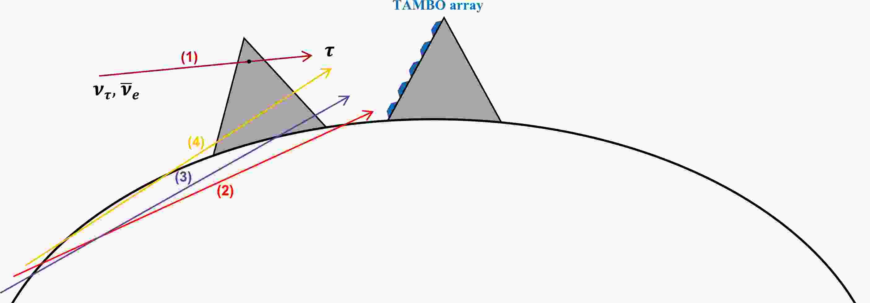
$ c \tau^{}_{\tau} \approx 50\; {\rm km}\cdot ({E^{}_{\tau}/{\rm EeV}}) $ , enabling the tau flux to emerge from the matter surface and decay to form extensive air showers. The air shower can then be measured by detecting radio waves, Cherenkov light, fluorescence, or direct shower particles, and key technologies have been significantly developed and adopted in cosmic ray and gamma ray experiments. One typical example is TAMBO [57], for which the particle detection array will be deployed on one side of a deep valley (like a highly inclined AUGER [79]), containing 22000 water tanks separated by$ 150\; {\rm m} $ each. By taking the valley length as$ 100\; {\rm km} $ and the array width as$ 5\; {\rm km} $ , the total geometric area of the telescope is as large as$ 500\; {\rm km}^2 $ . The Colca Valley in Peru, which has sufficient depth and length, is an ideal site to host the proposed array. The array will overwatch the other side of the valley by directly measuring shower particles induced by taus emerging from the matter surface.The detection volume of the telescope depends not only on the geometric area of the telescope but also on the tau energy. Only those taus that propagate out of the Earth before they decay can be measured. Generally speaking, the higher the tau energy, the larger the effective volume for generating observable taus from the Earth. The attenuation effect will also come into play when the cross section, which increases with the tau energy, is too large. The actual detection volume would then be a joint result of the telescope geography, the tau energy, and the matter attenuation effect. For a deep-valley telescope, there are primarily four kinds of events that define the path the primary neutrino has traveled through (depending on the incoming direction of the tau particles): (1) only mountain; (2) only Earth; (3) Earth and mountain; (4) Earth, air, and then mountain. A sketch is given in Fig. 1 to show these four possibilities for the particle trajectory. The particles that have traveled through the vast volume of Earth are referred to as "Earth-skimming neutrinos." The attenuation effect for Earth-skimming neutrinos is much stronger than that for neutrinos only traveling through the mountain.
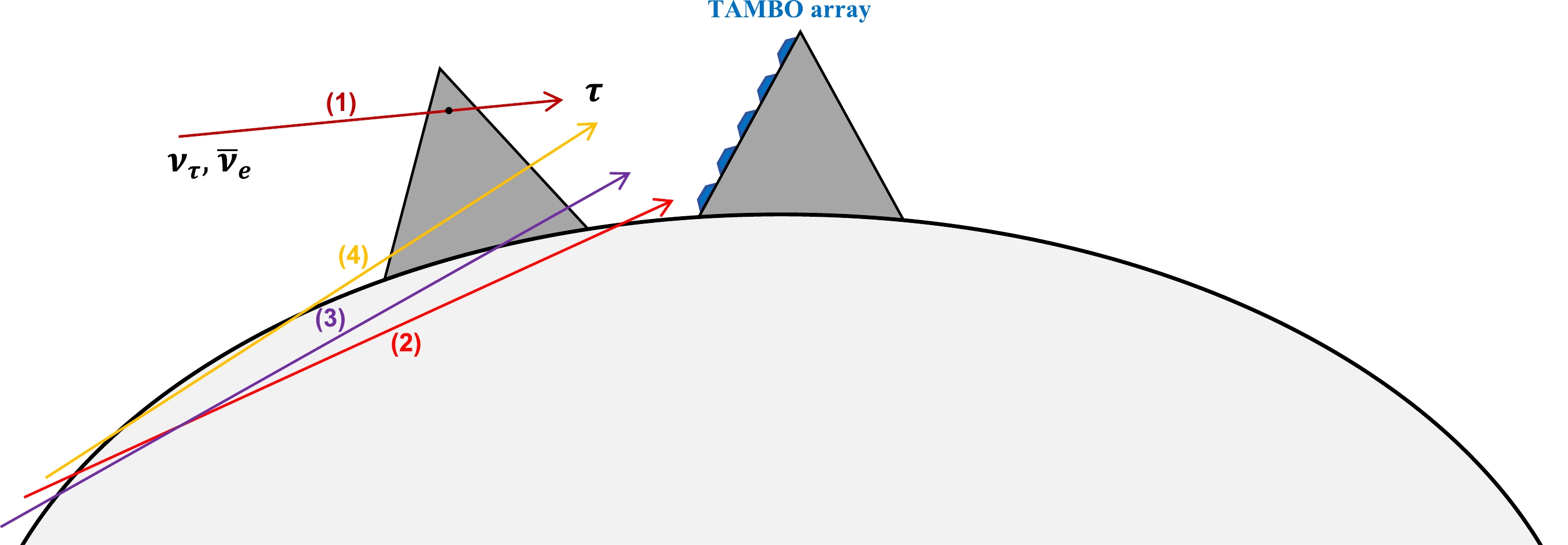
Figure 1. (color online) Schematic of the detection of neutrinos obtained by TAMBO. Four kinds of events in which incoming particles have traveled through different geographies are shown.
For this study, we developed our own numerical program to generate the events. Other excellent codes that solve the propagation of leptons in matter are available for public use, such as
$\mathrm{nuSQuIDS}$ [80],$\mathrm{NuTauSim}$ [81],$\mathrm{NuPropEarth}$ [82],$\mathrm{nuPyProp}$ [83],$\mathrm{PROPOSAL}$ [84] and,$\mathrm{TauRunner}$ [85, 86] . In our numerical calculation, we attempt to follow closely the configuration of TAMBO and simulate neutrino propagation and tau generation in matter. For the geography of the telescope, we adopt the cross sectional view in Fig. 5 of Ref. [57] and assume a valley length of$ 100\; {\rm km} $ , which is required to achieve the proposed sensitivity of TAMBO. There are valleys such as the Colca Canyon in Peru and the Yarlung Tsangpo Grand Canyon in China that can provide the required valley length of about 100 km [87]. We further assume that the mountain is composed of the standard rock and the Earth follows the PREM profile [88]. We follow Ref. [84] for the properties of the standard rock. The neutrino fluxes including$ \nu^{}_{\tau}/ \overline{\nu}^{}_{\tau} $ and$ \overline{\nu}^{}_{e} $ are then injected isotropically. The propagation equations in matter incorporating the Glashow resonance process are expressed as$ \begin{aligned}[b] \frac{\mathrm{d}}{\mathrm{d} t} \left(\frac{\mathrm{d}\Phi^{}_{{\nu}^{}_{\tau} + \overline{\nu}^{}_{\tau}} }{ \mathrm{d} E^{}_{\nu}} \right) = & - N^{}_{\rm A} \rho \left(\sigma^{}_{\rm CC} + \sigma^{}_{\rm NC} \right) \frac{\mathrm{d}\Phi^{}_{{\nu}^{}_{\tau} + \overline{\nu}^{}_{\tau}} }{ \mathrm{d} E^{}_{\nu}}\\ & + N^{}_{\rm A} \rho \int \mathrm{d} E^{\prime}_{\nu} \frac{\mathrm{d}\Phi^{}_{{\nu}^{}_{\tau} + \overline{\nu}^{}_{\tau}} }{ \mathrm{d} E^{\prime}_{\nu}} \frac{1}{E^{\prime}_{\nu} } \left.\frac{\mathrm{d}\sigma^{}_{\rm NC}}{\mathrm{d} z}\right|_{z = \frac{E^{}_{\nu}}{E^{\prime}_{\nu}} }\\ & + N^{}_{\rm A} \rho \frac{Z}{A} {\rm Br}^{}_{W\to \tau \overline{\nu}^{}_{\tau}} \int \mathrm{d} E^{\prime}_{\nu} \frac{\mathrm{d}\Phi^{}_{\overline{\nu}^{}_{e}} }{ \mathrm{d} E^{\prime}_{\nu}} \frac{1}{E^{\prime}_{\nu} } \left.\frac{ \mathrm{d}\sigma^{}_{\rm GR}}{\mathrm{d} z}\right|_{z = \frac{E^{}_{{\nu}}}{E^{\prime}_{\nu}} } \\ & + \int \mathrm{d} E^{\prime}_{ \tau} \frac{\mathrm{d} \Phi^{}_{\tau}}{\mathrm{d} E^{\prime}_{ \tau}} \frac{1}{E^{\prime}_{\tau}} \frac{\mathrm{d} \Gamma^{}_{\tau} }{ \Gamma^{}_{\tau} \mathrm{d} z} \;, \end{aligned} $

(1) $ \begin{aligned}[b] \frac{\mathrm{d}}{\mathrm{d} t} \left(\frac{\mathrm{d}\Phi^{}_{\overline{\nu}^{}_{e}} }{ \mathrm{d} E^{}_{\nu}} \right) = & - N^{}_{\rm A} \rho \left(\sigma^{}_{\rm CC} + \sigma^{}_{\rm NC} + \frac{Z}{A} \sigma^{}_{\rm GR} \right) \frac{\mathrm{d}\Phi^{}_{\overline{\nu}^{}_{e}} }{ \mathrm{d} E^{}_{\nu}} \\ & + N^{}_{\rm A} \rho \int \mathrm{d} E^{\prime}_{\nu} \frac{\mathrm{d}\Phi^{}_{\overline{\nu}^{}_{e}} }{ \mathrm{d} E^{\prime}_{\nu}} \frac{1}{E^{\prime}_{\nu} } \left.\frac{\mathrm{d}\sigma^{}_{\rm NC}}{\mathrm{d} z}\right|_{z = \frac{E^{}_{\nu}}{E^{\prime}_{\nu}} } \\ & + N^{}_{\rm A} \rho \frac{Z}{A} {\rm Br}^{}_{W\to e \overline{\nu}^{}_{e}} \int \mathrm{d} E^{\prime}_{\nu} \frac{\mathrm{d}\Phi^{}_{\overline{\nu}^{}_{e}} }{ \mathrm{d} E^{\prime}_{\nu}} \frac{1}{E^{\prime}_{\nu} } \left.\frac{ \mathrm{d}\sigma^{}_{\rm GR}}{\mathrm{d} z}\right|_{z = \frac{E^{}_{\nu}}{E^{\prime}_{\nu}} } \;, \end{aligned} $

(2) $ \begin{aligned}[b] \frac{\mathrm{d}}{\mathrm{d} t} \left(\frac{\mathrm{d}\Phi^{}_{\tau} }{ \mathrm{d} E^{}_{\tau}} \right) = & - \Gamma^{}_{\tau} \frac{\mathrm{d}\Phi^{}_{\tau} }{ \mathrm{d} E^{}_{\tau}} - \frac{N^{}_{\rm A}\rho}{A} \sigma^{}_{\rm \tau} \frac{\mathrm{d}\Phi^{}_{\tau} }{ \mathrm{d} E^{}_{\tau}} \\ & + \frac{N^{}_{\rm A}\rho}{A}\int \mathrm{d} E^{\prime}_{\tau} \frac{\mathrm{d}\Phi^{}_{\tau}}{\mathrm{d} E^{\prime}_{\tau}} \frac{1}{E^{\prime}_{\tau}} \frac{\mathrm{d} \sigma^{}_{\rm \tau} }{\mathrm{d} z} \\ & + \rho \frac{\partial}{\partial E^{}_{\tau}} \left( \beta^{}_{\tau} E^{}_{\tau} \frac{\mathrm{d}{\Phi^{}_{\tau}}}{\mathrm{d} E^{}_{\tau}} \right) \\ & + N^{}_{\rm A} \rho \int \mathrm{d} E^{\prime}_{\nu} \frac{\mathrm{d} \Phi^{}_{{\nu}^{}_{\tau} + \overline{\nu}^{}_{\tau}}}{\mathrm{d} E^{\prime}_{\nu}} \frac{1}{ E^{\prime}_{ \nu }} \frac{\mathrm{d}\sigma^{}_{\rm CC}}{\mathrm{d} z} \\ & + N^{}_{\rm A} \rho \frac{Z}{A} {\rm Br}^{}_{ W\to \tau \overline{\nu}^{}_{\tau} } \int \mathrm{d} E^{\prime}_{\nu} \frac{\mathrm{d}\Phi^{}_{\overline{\nu}^{}_{e}} }{ \mathrm{d} E^{\prime}_{\nu}} \frac{1}{E^{\prime}_{\nu} } \left.\frac{ \mathrm{d}\sigma^{}_{\rm GR}}{\mathrm{d} y}\right|_{y = \frac{E^{}_{\tau}}{E^{\prime}_{\nu}} }\;, \end{aligned} $

(3) where
$ N^{}_{\rm A} $ is the Avogadro constant; ρ is the matter density; Z is the atomic number; A is the mass number;$ \sigma^{}_{\rm CC} $ and$ \sigma^{}_{\rm NC} $ represent the DIS cross sections of the charged-current and neutral-current (NC) interactions, respectively;$ \Gamma^{}_{\tau} $ ,$ \sigma^{}_{\tau} $ , and$ \beta^{}_{\tau} $ describe the decay and the attenuation of tau in matter;$ \sigma^{}_{\rm GR} $ represents the cross section of the Glashow resonance (which takes a Breit-Wigner form); and${\rm Br}^{}_{W\to\tau \overline{\nu}^{}_{\tau}} \approx {\rm Br}^{}_{W\to e \overline{\nu}^{}_{e}} \approx 11$ % are the branching ratios of the decay channels of interest. The differential cross section of the resonant scattering reads$ \mathrm{d}\sigma^{}_{\rm GR}/{\mathrm{d} y} = \sigma^{}_{\rm GR} \cdot 3 (1-y)^2 $ , where$ y \equiv E^{}_{\tau} / E^{\prime}_{\nu} $ is the energy fraction of the daughter tau taken from the primary neutrino [41]. The secondary$ \nu^{}_{e} $ and$ \nu^{}_{\mu} $ from tau decays are not included in the above equations, which only have a subleading effect [85, 86, 89, 90].Owing to the angular momentum conservation, the average fraction of energy carried by the daughter tau from W is suppressed; specifically,
$\langle y \rangle \sim 25$ % in comparison with$\langle y \rangle \sim 80$ % for the DIS CC interaction. This reduces the detection volume of the Glashow resonance by a factor of three, as compared to the normal tau neutrino events for the same primary neutrino energy. The detection volume is further reduced because of the large cross section (i.e.,$ \sigma^{\rm max}_{\rm GR} \approx 5 \times 10^{-31}\; {\rm cm^2} $ ), which corresponds to an attenuation length of$ L^{}_{\rm GR} \approx 30 \; {\rm km} $ in the standard rock. Hence, the attenuation effect signficantly decreases the event number for the upward going Earth-skimming neutrinos, which traverse a distance much longer than$ L^{}_{\rm GR} $ .By solving the propagation equations, one can obtain the tau flux emerging from the matter surface and then simulate their decays in the air. For simplicity, we assume that the detector will be triggered as long as the air shower axis intersects with the area covered by the array. This is a rather optimistic assumption, especially for less energetic neutrinos. In practice, one has to perform Monte-Carlo simulations for the development of extensive air showers and event registration in water tanks. The detector may not be triggered if the shower energy is too low. Nonetheless, our result presented here should be regarded as the most optimistic limit that may be reached by further improving the detection threshold. We will show later that it is still statistically difficult to identify the Glashow resonance in such an ideal case. Incorporating the practical shower simulation should further reduce the discovery potential.
Using the framework above, we can first check the sensitivity of our nominal telescope to the diffuse neutrino flux. In Fig. 2, we show the acceptance (upper panel) and the sensitivity (lower panel) at the
$90$ % CL for$ \nu^{}_{\tau}/\overline{\nu}^{}_{\tau} $ (dark blue curves) via DIS and$ \overline{\nu}^{}_{e} $ (red curves) via the Glashow resonance based on our simulation. The sensitivity to the all-flavor neutrino flux is obtained by requiring the differential event number per energy decade to be greater than 2.44 for the$90$ % CL and assuming a democratic flavor composition along with$ \nu^{}_{e}:\overline{\nu}^{}_{e} = 0:1 $ . For comparison, the dashed purple curve represents the acceptance and the corresponding sensitivity of the original TAMBO proposal to$ \nu^{}_{\tau}/\overline{\nu}^{}_{\tau} $ [57]. The result of our ideal simulation is very similar to the TAMBO curve and starts to deviate significantly when the neutrino energy is below the PeV level. This deviation indicates that the energy threshold of TAMBO is important for$ E^{}_{\nu} \lesssim \mathcal{O}(\rm PeV) $ , above which the detector can accept tau events at almost full efficiency. The sensitivity to$ \overline{\nu}^{}_{e} $ with the Glashow resonance can exceed that to$ \nu^{}_{\tau}/\overline{\nu}^{}_{\tau} $ in a narrow energy window around$ E^{}_{\nu} \approx 6.3\; {\rm PeV} $ . However, the actual event number from the Glashow resonance is subject to an integration over the input neutrino flux.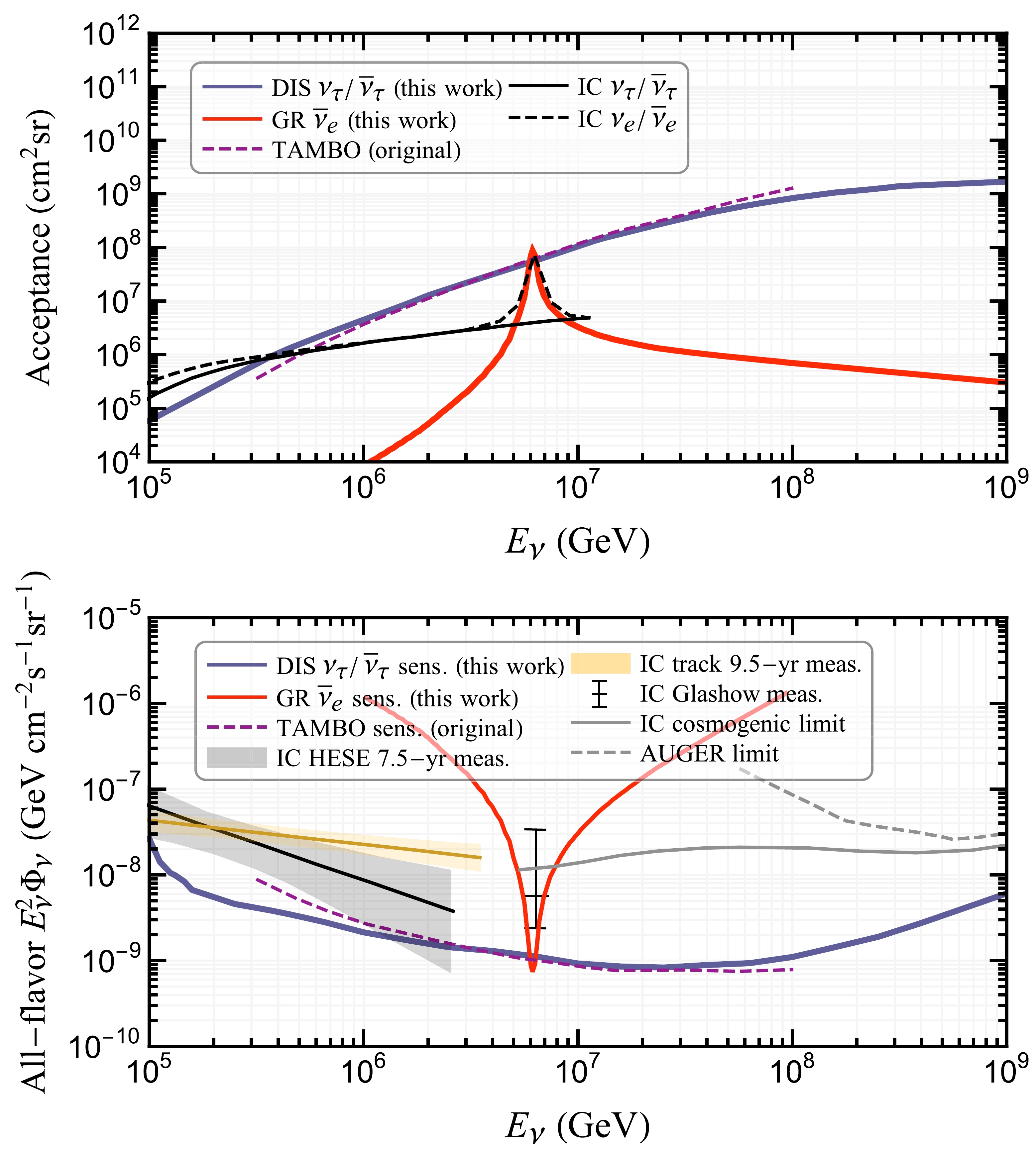
Figure 2. (color online) Acceptance (upper panel) and 10-year sensitivity (lower panel) of our nominal neutrino telescope to
$ \nu^{}_{\tau}/\overline{\nu}^{}_{\tau} $ (dark blue curves) via DIS and to$ \overline{\nu}^{}_{e} $ (red curves) via the Glashow resonance. This nominal setup closely follows the TAMBO proposal [57], of which the original acceptance and sensitivity to$ \nu^{}_{\tau}/\overline{\nu}^{}_{\tau} $ are given in purple curves. In the upper panel, acceptances of IceCube to$ \nu^{}_{\tau}/\overline{\nu}^{}_{\tau} $ and$ \overline{\nu}^{}_{e} $ are shown for comparison [24]. In the lower panel, several experimental results on the diffuse neutrino flux are given, including the measurements from the IceCube 7.5-year HESE data [27], 9.5-year northern sky track data [91], and one Glashow resonance candidate [2], as well as the limits from the IceCube [92] and AUGER [93] searches for cosmogenic neutrinos.For comparison, several existing results are shown: the IceCube sensitivity to
$ \nu^{}_{\tau}/\overline{\nu}^{}_{\tau} $ (solid black curve) and$ \overline{\nu}^{}_{e} $ (dashed black curve) via both DIS and the Glashow resonance [24], the IceCube measurements on the diffuse neutrino flux with 7.5-year HESE data (gray band) [27] and 9.5-year through-going track data (orange band) [91], the flux estimate from the IceCube Glashow resonance candidate (black error bar) [2], and the cosmogenic neutrino searches by IceCube (solid gray curve) [92] and AUGER (dashed gray curve) [93]. TAMBO's sensitivity to$ \nu^{}_{\tau}/\overline{\nu}^{}_{\tau} $ is better than that of IceCube by more than one order of magnitude above$ \mathcal{O}(10\; {\rm PeV}) $ . However, its sensitivity to$ \overline{\nu}^{}_{e} $ via the Glashow resonance is almost comparable to that of IceCube owing to the aforementioned suppression of the detection volume. -
We continue with investigating the potential of air shower neutrino telescopes for detecting the Glashow resonance by comparing event numbers and distributions of both the signal and background. As has been mentioned, the major background signal comes from the irreducible tau neutrino events, which have the same event topology as the Glashow resonance signal in the air shower neutrino telescope. The only feasible way to identify the Glashow resonance seems to be statistically analyzing event distributions. Owing to neutrino oscillations, there will always be a comparable tau neutrino component no matter what the initial neutrino flavor ratio is at the source [94−110]. For instance, the initial flavor ratios for the proton-proton (pp) and proton-photon (pγ) sources are both around
$ \nu^{}_{e} + \overline{\nu}^{}_{e} : \nu^{}_{\mu} + \overline{\nu}^{}_{\mu} : \nu^{}_{\tau} + \overline{\nu}^{}_{\tau} = 1:2:0 $ , which leads to a nearly democratic flavor composition$ \approx 1:1:1 $ at Earth. In the following demonstrations, unless otherwise specified, the flavor ratio is set to$ 1:1:1 $ with an optimistic input$ \nu^{}_{e}:\overline{\nu}^{}_{e} = 0:1 $ .In an in-ice or in-water Cherenkov telescope such as IceCube, the Glashow resonance stands out as a hadronic cascade with an energy deposition close to
$ E^{}_{\rm dep} \sim 6.3\; {\rm PeV} $ . In the narrow energy window of interest, the background contribution from DIS is very low. However, this is not the case for the air shower neutrino telescope, which is designed to detect the tau lepton only. The resonance bump is largely smoothed out because of the wide spread of the tau energy from$ 0\; {\rm PeV} $ to$ 6.3\; {\rm PeV} $ . To see this explicitly, in Fig. 3 we show the energy (left panel) and angular (right panel) distributions of tau events in the telescope with ten years of exposure. The upper panels show the differential event distributions on a logarithmic scale and the lower ones give the event numbers collected in each bin. The red curves and regions depict the Glashow resonance events while the blue ones represent the tau neutrino events. For illustration, we have used as the input a power-law neutrino spectrum, which is expressed as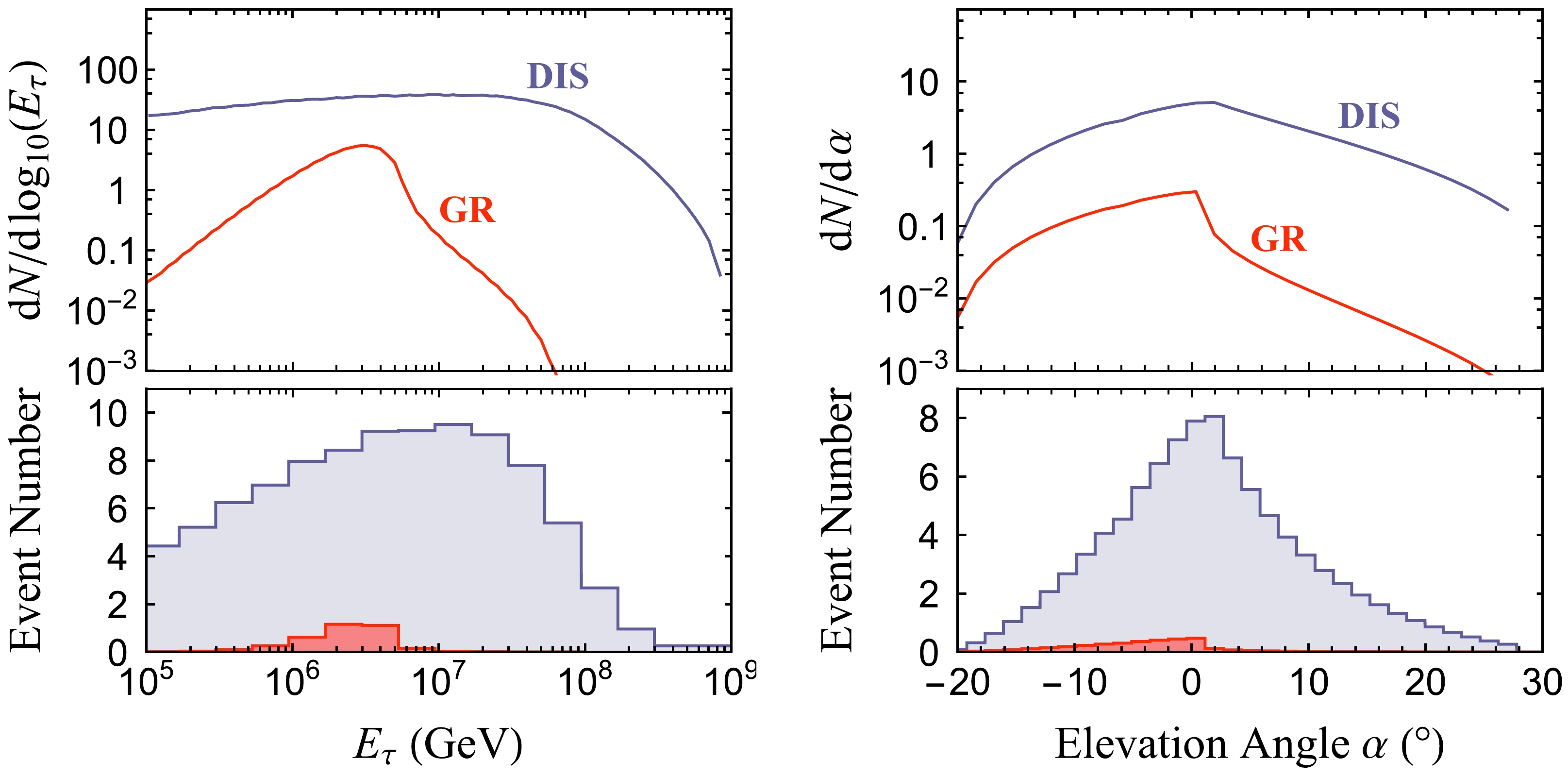
Figure 3. Event distributions (upper panels) and numbers (lower panels) in terms of the tau energy
$ E^{}_{\tau} $ (left panel) and the incoming elevation angle α (right panel), assuming 10 years of data collection. The Glashow resonance and tau neutrino events are shown in red and blue, respectively. The power-law neutrino spectrum in Eq. (4) with$ {\rm \Phi}= 4.32 $ and$ \gamma = 2.28 $ was used as the input.$ \frac{\mathrm{d} {\rm \Phi}^{}_{6\nu}}{\mathrm{d} E^{}_{\nu}} = {\rm \Phi} \left(\frac{E^{}_{\nu}}{100\; {\rm TeV}}\right)^{-\gamma}10^{-18}\; {\rm GeV^{-1} cm^{-2} s^{-1} sr^{-1}} \;, $

(4) with
$ {\rm \Phi}= 4.32 $ and$ \gamma = 2.28 $ (i.e., the best-fit values of IceCube's 9.5-year track data [91]). The elevation angle in the right panel is defined as$ \alpha \equiv \theta-90^{\circ} $ , where θ is the zenith angle of a neutrino's incoming direction, with the z-axis pointing upwards. Further remarks on Fig. 3 are made below.● For the chosen flux parameters, the expectation number for the Glashow resonance events with 10 years of data collection was found to be
$ N_{\rm GR} \approx 2.9 $ , which is promising for observations if we could reject the background (i.e., tau neutrinos). The background event number shall be counted within a given region of interest (ROI). As shown in the left panel of Fig. 3, even though the resonance cross section features a very narrow width, the energy distribution of tau events spreads over a wide range. We found that the event number of the Glashow resonance peaked around$ E_{\tau} \approx 2.2\; {\rm PeV} $ with a large standard deviation in the energy of$\Delta \ln(E_{\tau}) \equiv \Delta E_{\tau}/E_{\tau} \approx 70$ %, corresponding to an energy interval of$E_{\tau} \in \left[1.1,\; 4.5\right]\; {\rm PeV}$ . This energy interval is suitable for consideration as the ROI in order to optimize the signal-to-background ratio: for a wider interval one may involve too many background events compared to the signal, while for a narrower interval the signal events may not be sufficiently taken into account.● However, the angular distribution in the right panel motivates us to impose a
$ \alpha< 2^{\circ} $ cut to reduce the background. As we have mentioned, the Glashow resonance events for Earth-skimming neutrinos ($ \alpha \gtrsim 2^{\circ} $ ) are strongly suppressed because of attenuation. The angular cut will reduce the background event number by approximately a factor of two, and the signal will be almost unchanged. After the angular cut, the background event number within the ROI turns out to be$ N_{\rm DIS} \approx 10 $ with a$ 1\sigma $ fluctuation of$ \sqrt{N_{\rm DIS}} \approx 3.2 $ , which is just comparable to$ N_{\rm GR} $ . This implies that the signal significance is only around the$ 1\sigma $ CL for the assumed flux input.● In practice, the ROI choice is further limited by the energy resolution of taus in the telescope. For the TAMBO proposal, the target energy resolution is around
$\Delta E_{\tau}/E_{\tau} \approx 100$ % [57], which will contribute an additional smearing effect on top of the intrinsic energy spread.For the above example, we have fixed the flux normalization Φ and spectral index γ to be the best-fit values for IceCube track data. To be more general, we now set them as free parameters and perform the scanning. The event numbers of the signal and background in terms of Φ and γ are given in Fig. 4. In each panel, the parameter regions preferred by IceCube's HESE [27] and through-going track data [91] are shown as the solid contours (at the
$ 2\sigma $ CL) and stars (best fits). To maximize the signal-to-background ratio, the angular cut$ \alpha <2^{\circ} $ has been imposed. For illustration, we have chosen three different ROIs for calculating the event numbers, including$ E^{}_{\tau} \in \left[0.5,\; 9.2 \right]\; {\rm PeV} $ ,$ \left[1.1,\; 4.5 \right]\; {\rm PeV} $ , and$ \left[1.6,\; 3.2 \right]\; {\rm PeV} $ (top, middle, and bottom panels, respectively), which correspond to multiplying the standard deviation of the tau energy distribution by a factor of two, one, and half, respectively. For a large fraction of the parameter space favored by HESE data, the event number of the Glashow resonance is small,$ N^{}_{\rm GR} \lesssim 1 $ . For the parameter space favored by track data, a larger event number can be obtained, but the ratio$ N^{}_{\rm GR}/\sqrt{N^{}_{\rm DIS}} \lesssim 1 $ is not sufficient to claim that the signal is significant against the background.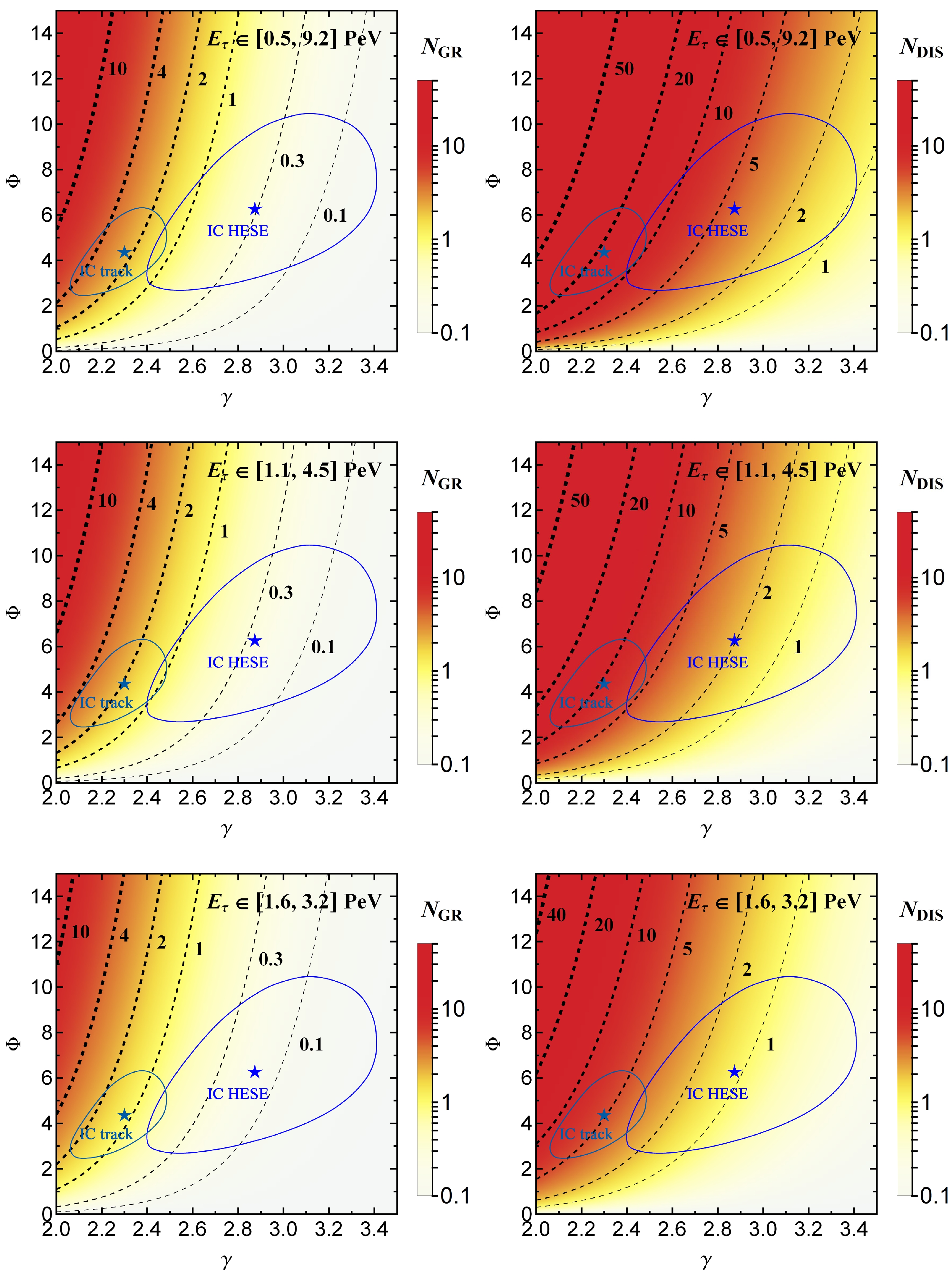
Figure 4. (color online) Event numbers within different energy intervals through the Glashow resonance (left panels) and DIS (right panels), assuming 10 years of data collection. For comparison, the parameter regions preferred by IceCube's HESE and track data are shown as the solid contours (at the
$ 2\sigma $ CL) and stars (best fits).When the flux normalization is too small or the spectrum is too soft,
$ N^{}_{\rm DIS} $ within the ROI can be of$ \mathcal{O}(1) $ , in which case$ N^{}_{\rm GR}/\sqrt{N^{}_{\rm DIS}} $ is no longer a good estimate for the signal significance. To accommodate all cases, we treat the event fluctuation according to the Poisson distribution, for which the probability distribution function (PDF) follows$ {\rm PDF}^{}_{\rm Poisson} (n, \mu) = e^{-\mu} \mu^n / {n!} $ , where μ is the expectation value and n is the number of counts. The corresponding cumulative distribution function (CDF) is defined as$ {\rm CDF}^{}_{\rm Poisson} (n, \mu) \equiv \sum^n_{k = 0} {\rm PDF}^{}_{\rm Poisson} (k, \mu) $ , and$ \overline{\rm CDF}^{}_{\rm Poisson} = 1 - {\rm CDF}^{}_{\rm Poisson} $ is its complementary function. To define the discovery probability of the signal, we can perform a set of pseudo-experiments, and calculate the p-value that a fraction of pseudo-experiments can exclude the null (background-only) hypothesis. The p-value can be derived by solving [111]$ p = {\rm CDF}^{}_{\rm Poisson} (n^{}_{p }, N^{}_{\rm DIS}) \; ,\; \overline{\rm CDF}^{}_{\rm Poisson} (n^{}_{p }, N^{}_{\rm DIS} + N^{}_{\rm GR}) = q \; , $

(5) where
$ n^{}_{p } $ is the mock event number that can be observed by a fraction q of pseudo-experiments including both signal and background events. The median sensitivity corresponding to$q = 50$ % is assumed, so that p quantifies the significance that half of the pseudo-experiments can exclude the null hypothesis. For illustration, we have smoothed over the CDF by taking$ {\rm CDF}^{}_{\rm Poisson} (x, \mu) = \Gamma(x+1,\mu)/\Gamma(x+1) $ with$ x \in \mathbb{R} $ , following Ref. [112].In the upper panels of Fig. 5, we show the p-value in terms of
$ {\rm \Phi} $ and γ for the flavor composition$ \nu^{}_{e} + \overline{\nu}^{}_{e} : \nu^{}_{\mu} + \overline{\nu}^{}_{\mu} : \nu^{}_{\tau} + \overline{\nu}^{}_{\tau} = 1:1:1 $ consistent with meson-decay neutrino sources, with$ \nu^{}_{e}:\overline{\nu}^{}_{e} = 0:1 $ . In each panel, the confidence levels of$p = 68$ % and$90$ % are indicated by the dashed contours. If the event number is completely consistent with the background-only hypothesis, then$p \approx 50$ %. The significance that results after choosing$ E^{}_{\tau} \in \left[1.1,\; 4.5\right]\; {\rm PeV} $ was the best among the three ROI choices. However, a$90$ % CL cannot be achieved for the flux parameters constrained by the IceCube data. The largest p-value we found within the allowed region of neutrino flux was around$82$ %.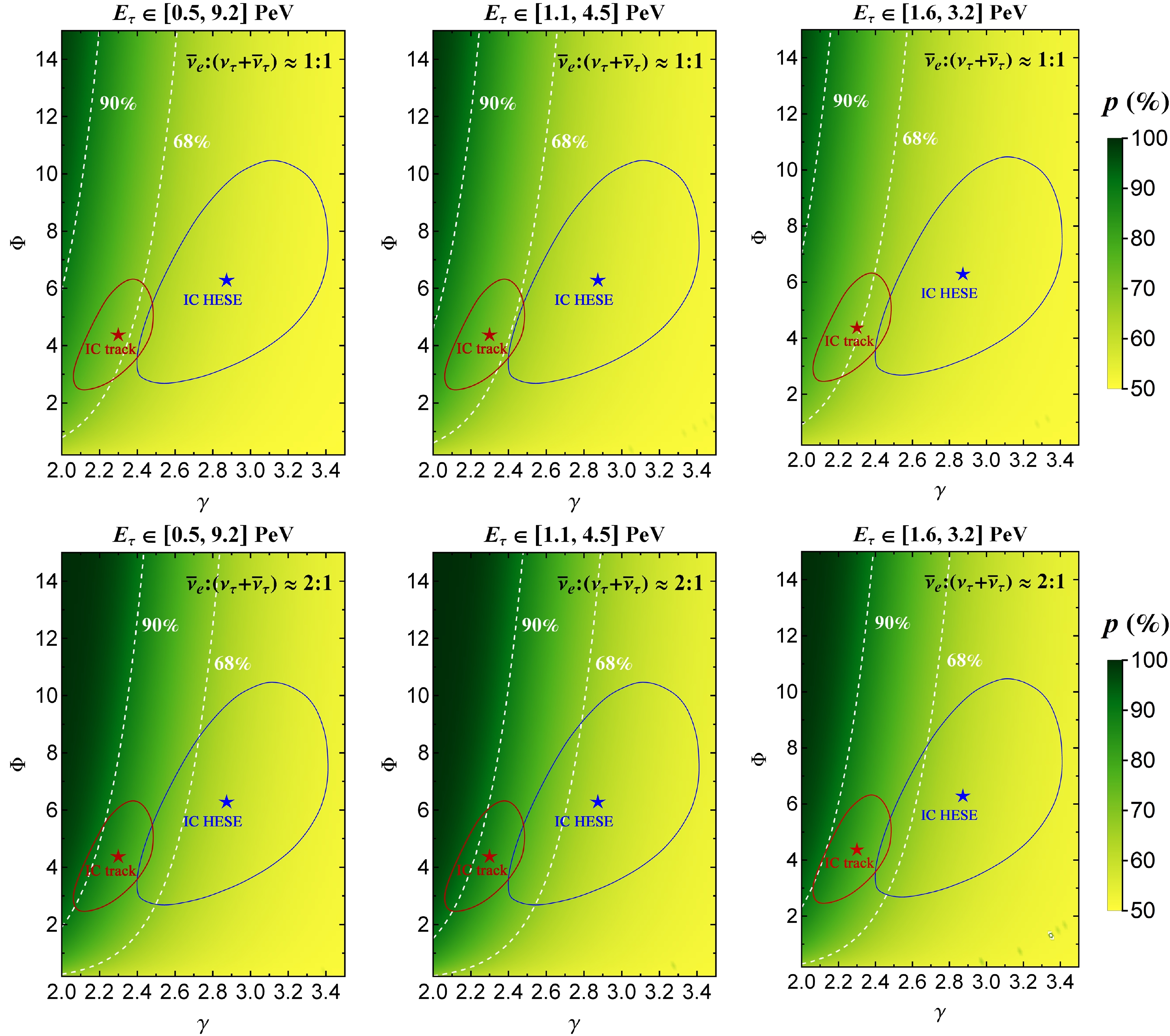
Figure 5. (color online) The p-value to exclude the null-signal hypothesis (DIS background only) with different energy intervals in the plane of Φ and γ, assuming an exposure of 10 years. In the upper and lower panels, the flavor ratio
$ \nu^{}_{e} + \overline{\nu}^{}_{e} : \nu^{}_{\mu} + \overline{\nu}^{}_{\mu} : \nu^{}_{\tau} + \overline{\nu}^{}_{\tau} $ at Earth has been taken as$ 1:1:1 $ (for meson decays) and$ 0.55:0.17:0.28 $ (for neutron decays), respectively.A more optimistic scenario is that the incoming tau neutrino component is suppressed. An example is the neutron-decay origin of UHE neutrinos, where only
$ \overline{\nu}^{}_{e} $ is produced at the source, and after oscillations, one roughly obtains$ \nu^{}_{e} + \overline{\nu}^{}_{e} : \nu^{}_{\mu} + \overline{\nu}^{}_{\mu} : \nu^{}_{\tau} + \overline{\nu}^{}_{\tau} = 0.55:0.17:0.28 $ with$ \nu^{}_{e}:\overline{\nu}^{}_{e} = 0:1 $ at Earth [110]. In this scenario, the$ \overline{\nu}^{}_{e} $ flux is nearly twice that of the$ \nu^{}_{\tau} + \overline{\nu}^{}_{\tau} $ flux. In the lower panels of Fig. 5, we show the p-value of the Glashow resonance discovery for the neutron-decay origin. A$ 90\ $ % CL can be reached within the allowed region of the neutrino flux. However, the neutron-decay scenario is not favored as the dominant source of UHE neutrinos because of less energetic neutrinos in the final state. -
In the air shower neutrino telescope, the major difficulty in extracting the Glashow resonance signal stems from the original tau neutrino events, which contribute an intrinsic background to the resonance events. Even though the Glashow resonance process can induce an observable event excess within an energy window, discriminating the Glashow resonance from the tau neutrino background is statistically challenging if UHE neutrinos primarily come from meson decays at the source. We have identified several factors that limit the discovery potential: (i) the small branching ratio of the decay
$ W \to \tau\nu^{}_{\tau} $ ; (ii) the spreading energy distribution of the final-state tau as well as the sizable energy resolution; and (iii) the attenuation effect for upward going Earth-skimming neutrinos. Cosmic tau neutrinos remain the most cost-effective scientific target of the air shower neutrino telescope. Nevertheless, identifying the Glashow resonance is promising if UHE neutrinos are of the less likely neutron-decay origin or some new physics can come into play to suppress the tau neutrino component at Earth [99, 100, 113].Our result described above is more or less optimistic. In a more complete analysis, the neutrino flux input itself is uncertain and should be fitted by the data. The flux uncertainty will to some extent dilute the sensitivity to the bump induced by the Glashow resonance. In the TAMBO-like setup, to disentangle the flux uncertainty one may first fix the tau neutrino spectrum by using the Earth-skimming events (
$ \alpha \gtrsim 0^{\circ} $ ), and then use it to generate the background expectation for the horizontal ($ \alpha \lesssim 0^{\circ} $ ) events. The measurements gathered by other UHE neutrino telescopes can also be used as the input to further reduce the flux uncertainty. The TAMBO-like setup may be scaled up by deploying the arrays at multiple sites. The valleys that have been considered as the host for TAMBO include the Hells Canyon, Yarlung Tsangpo Grand Canyon, Cotahuasi Canyon, and Colca Canyon. Neglecting the cost budget, simply rescaling the length of the toy valley to$ 1000\; {\rm km} $ will enable a geometric area of$ 5000\; {\rm km^2} $ to be achieved. With a sufficiently large ensemble of statistics, this will make the discrimination of the Glashow resonance possible ($ \sim 2\sigma $ CL) even for meson-decay neutrino sources. -
The author would like to thank Ting Cheng, Sudip Jana and Nele Volmer for helpful comments and discussions.
Discovery potential of the Glashow resonance in an air shower neutrino telescope
- Received Date: 2024-04-02
- Available Online: 2024-08-15
Abstract: The in-ice or in-water Cherenkov neutrino telescope, such as IceCube, has already proved its power in measuring the Glashow resonance by searching for the bump around


 DownLoad: