


 Abstract
 HTML
HTML Reference
 Related
 PDF
PDF


-
The interplay between the chiral anomaly and external electromagnetic or vortical fields can lead to intriguing anomalous transport phenomena in many-body systems with chiral fermions. A notable example is the chiral magnetic effect (CME) [1, 2], which induces an electric current aligned with an external magnetic field. In heavy-ion collisions, the CME may cause charge separation relative to the reaction plane, which can potentially be observed by analyzing the azimuthal-angle distribution of charged hadrons using specific observables [3, 4]. Other notable anomalous transports include the chiral separation effect (CSE) [5, 6], the chiral vortical effect [7–10], and the chiral electric separation effect (CESE) [11, 12]. For reviews, see Refs. [13–17].
In the presence of an external magnetic field, the coupled evolution of CME and CSE gives rise to a gapless collective mode known as the chiral magnetic wave (CMW) [18]. The CMW can transfer both chirality and electric charge, potentially resulting in distinct charge and chirality distributions. In heavy-ion collisions, the fireball contains a small amount of positive charges inherited from the colliding nuclei. Thus, theoretical studies have suggested that the CMW can induce a charge quadrupole in the fireball, with an accumulation of positive charges at the tips and negative charges around the equator. As the fireball expands, this quadrupole leads to an imbalance in the elliptic flow of charged pions, specifically
$ v_2(\pi^-) > v_2(\pi^+) $ [19]. Owing to event-by-event fluctuation of charges, some events could have net negative charges in the fireball, thereby leading to$ v_2(\pi^-) < v_2(\pi^+) $ . This characteristic feature of CMW provides a method to detect it in heavy-ion collisions, and a series of experiments have found signals of charged pion elliptic flow consistent with CMW expectations [20–24]. However, similar to CME, CMW in heavy-ion collisions faces strong background noise [25–31], which significantly obscures the observables designed for CMW detection.In Ref. [38], we developed a CME-meter based on convolutional neural networks (CNNs) (for reviews of deep learning techniques applied to nuclear physics, see Refs. [32–35]). After training this CME-meter with AMPT-generated data simulating CME (introducing an initial charge separation into the AMPT model [36]) for Au + Au collisions at 200 GeV, the CME-meter demonstrated exceptional robustness in distinguishing events with CME from those without. Additionally, the CME-meter maintained strong performance across different charge separation fractions, collision energies, and collision systems. This success suggests potential for creating a similar CMW-meter. As an extension of our earlier work, we aimed to increase the upper limit of salience at the cost of some generalization capability. This approach could pave the way for future studies on CMW physics and its detection.
In this paper, we report on the construction and performance of such a CMW-meter. Section II details the training process, including the generation of training samples using AMPT, the structure of the neural network, and the training procedure. Section III examines the analysis of the trained model, including its basic properties, comparisons to flows and observables, and a hypothesis test. Section IV provides a summary of our findings.
-
In this section, we introduce the deep learning model, data set preparation, and training strategies employed in constructing the CMW-meter. The pion spectra of heavy-ion collision final states serve as the input of this deep learning model. Pions carry most of the electric charges in the final state, establishing an appropriate representation of charge distribution. A convolutional neural network (CNN) was trained within a supervised learning scheme to identify the CMW signals. The training data were generated from the string-melting AMPT model [36], a transport model which is widely used to simulate the evolution of both partonic and hadronic matter in heavy-ion collisions.
To incorporate the CMW effect into the AMPT model, we adopted a global charge quadrupole scheme introduced in Ref. [37]. For an AMPT event with
$ A_{\rm{ch}}>-0.01 $ , we propose to interchange the positions of certain u (or$ \bar{d} $ ) quarks in the initial state with those of$ \bar{u} $ (or d) quarks if the former are relatively farther from the reaction plane (RP); for events with$ A_{\rm{ch}}<-0.01 $ , we propose to do the opposite. Here,$ A_{\rm{ch}} $ denotes the asymmetry of the charged particle number, given by$A_{\rm{ch}} = (N^+-N^-)/ (N^++N^-)$ , where$ N^+ $ denotes the number of positively charged particles measured in a given event, and$ N^- $ denotes negatively charged particles. The RP of all events is set in the$ zOx- $ plane. The fraction of particles that are interchanged is represented by a relative percentage with respect to the total number of quarks,$ f = \frac{\#\ {\rm{Exchanged\ particles}}}{\#\ {\rm{All\ particles}}}. $

(1) According to a previous study [37], switching
$f= 2{\text{%}}-3{\text{%}}$ of quarks generates a CMW signal comparable to experimental observables. For training and validation purposes, we chose events with a$ f=2$ % switching fraction. The transition point$ A_{\rm{ch}}=-0.01 $ in this scheme is based on STAR experimental results [20], where more details are provided. Events at$ \sqrt{s_{NN}}=200$ GeV and different centrality were generated for training and validation.There are two primary reasons for training a model that results in bias and overfitting at 200 GeV. First, the pivotal issue pertains to the occurrence of CMW in heavy-ion collisions rather than to the magnitude of the signal. Consequently, any technique that can distinctly distinguish CMW signals from background noise is considered valuable, irrespective of the
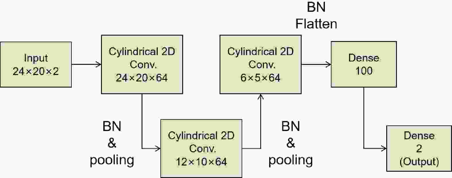
$ \sqrt{s_{NN}} $ or event centrality. Second, our research on the application of neural networks for CME detection [38] confirmed the robustness of the trained network against variations in collision energy and event centrality. The training was successful on the most comprehensive dataset, demonstrating high accuracy levels. Only small variance in the detection performance of the network was observed from such variations. Therefore, a model trained on a single energy is capable of enhancing the signal detection in certain events while still maintaining a considerable degree of generalization. However, further examinations involving various energies and centralities have also been conducted to provide a more nuanced analysis. The structure of the CNN used in this study is shown in Fig. 1. It includes three 2D-convolutional layers and two dense layers that contain parameters to be fit. Some pooling layers are also included for proper data reduction while keeping the network simple. To encode ''knowledge" about CMW in the model, samples with and without CMW, labeled as '1' and '0' separately, were fed to it during training, and the model was set to classify these samples. The last activation function of the network is SoftMax, which returns a pair of numbers$ (P_0,\,P_1) $ for this binary classification problem. Samples with$ P_1>0.5 $ are categorized as class '1'; otherwise, they are categorized as class '0'. Therefore,$ P_1 $ can be interpreted as the probability that a specific sample be recognized by the neural network as containing the CMW signal.
Figure 1. (color online) A VGG-like network [39] with four hidden layers was chosen for this study. Batch normalization (BN) is applied after each hidden layer. The convolutional layers were modified to satisfy the periodic boundary condition of the input data; each layer is followed by an average pooling. A 10% dropout was set for the second-to-last dense layer.
Data pre-processing involved several steps to convert events into analyzable samples. Initially, the spectra for mid-rapidity (
$ |\eta|<1 $ ) pions, denoted as$ \rho^\pm(p_T, \phi) $ , were calculated, with the symbol$ \pm $ representing either$ \pi^+ $ or$ \pi^- $ , while$ p_T $ denotes the transverse momentum in the range of$ 0-2 $ GeV and ϕ indicates the azimuthal angle. These spectra were then segmented into histograms consisting of 20 by 24 bins. Second, each spectrum was normalized so that the sum of all bins became 1. Subsequently, a random selection of events was made, and for each type of pion, their spectra were averaged bin by bin. These resulting normalized and averaged pion spectra served as the datasets for the training, validation, and testing phases of the neural network. Unless otherwise stated, the number of events in the last step is assumed to be 100 in the rest of this article. The training of the model encompassed 250 epochs, with each epoch containing 64 batches, and each batch comprising 100 samples. A total of 1.6 million samples were generated for training. -
Accuracy, robustness, and extrapolations.— As mentioned above, the model was trained (and also validated) on samples generated at
$ \sqrt{s_{NN}}=200$ GeV that mimic final-state CMW behavior. The model achieves high accuracy on most events with signal at different$ \sqrt{s_{NN}} $ and centrality, as shown in Fig. 2. This indicates preferable generalization of the trained model. Reduction of accuracy was observed at low collision energy and large centrality. The reasons for this are varied. Different patterns of CMW, weaker signals, stronger backgrounds or just overfitting, all of them can account for the reduction of accuracy. One of the approches to detect CMW in experiments is based on the dependency of charge distribution and flow analysis. Specifically, the linear order dependency of$ A_{\rm{ch}} $ on the difference in charged-particle elliptic flow,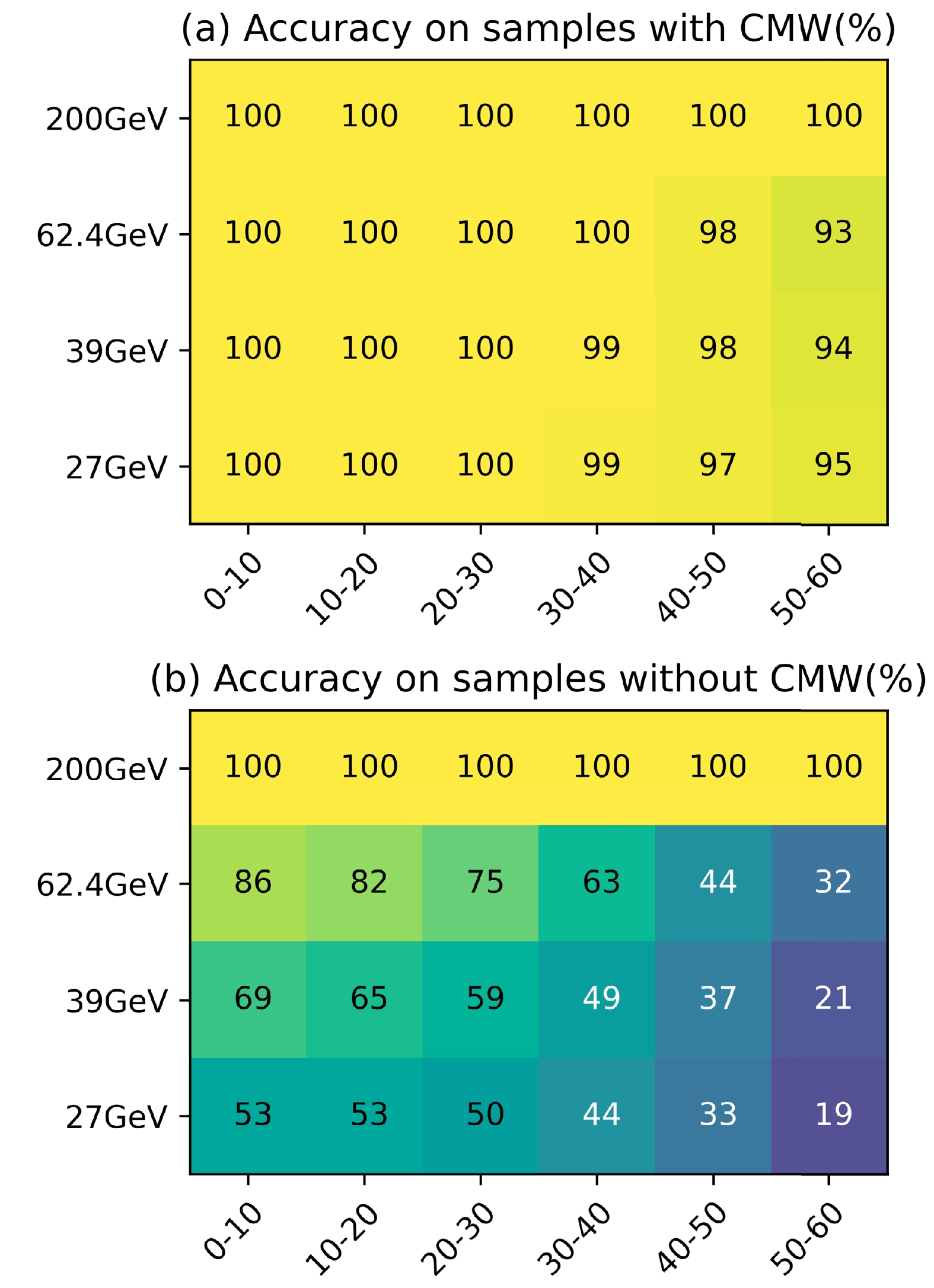
Figure 2. (color online) Accuracy of the trained model on samples (a) with CMW, and (b) without CMW. Samples from various
$ \sqrt{s_{NN}} $ and centralities are considered. The accuracy is remarkably high if the signal is encoded in the samples, while those without signal can be mistaken as containing it, especially at lower energy and for more peripheral cases.$ \Delta v_2 \equiv v_2^- - v_2^+ \simeq r A_{\rm{ch}}, $

(2) gives a measure for the CMW signal. Here,
$ v_2^- $ and$ v_2^+ $ are separate elliptic flows of negative- and positive-charge particles, and the slope r is related to the strength of the signal. Experimental results from the STAR experiment for Au + Au collisions [23] indicate that the uncertainty of the π slope r increases at lower energies and higher centralities. Although the neural network was trained on pions from a larger kinematic window than that used in experimental analyses, which suggests improved completeness and distinguishing capability, its performance aligns with traditional statistical analysis trends ($ \Delta v_2 (\pi) $ ). The decrease in accuracy is likely due to strong backgrounds in scenarios that compare with the signal strength. However, a new model can be trained using low-energy samples or in combination with high-energy samples to create a more comprehensive training set, enhancing robustness. This approach is left for a future, more detailed study. Overall, the accuracy of the trained model in decoding the CMW signal is sufficient across all tested$ \sqrt{s_{NN}} $ levels, especially on high-energy samples.As a potential detector for CMW, a measure of performance is the prediction on non-labeled samples, where accuracy cannot be defined, and the sample-by-sample output becomes important. The two components of the model output are identified as probabilities, i.e.,
$ P_1 $ denotes the probability that the neural network regards the input spectrum to include CMW, and$ P_0 $ is the probability associated to the other class; thus, the two components jointly satisfy$ P_0+P_1=1 $ . A positive correlation of$ P_1 $ with the CMW signal is clearly expected. Events with different initial charge quadrupole fractions f were simulated and prepared into samples as mentioned above. Tests on these samples resulted in high true-positive accuracy, yet the returned$ P_1 $ values for all f were close to 1, which means small differences among them. For the sake of a clear comparison, we enlarged the differences of their output by introducing an additional logit function,$ {\rm{logit}}(x)={\rm{log}}\frac{x}{1-x}\,. $

(3) This logit function, which is the inverse function of SoftMax, acting on
$ P_1 $ reveals feature space information that is encoded in the neural network one layer before output. Besides, the logit function is monotonically increasing, so logit($ P_1 $ ) keeps the correlation of$ P_1 $ and f qualitatively.Figure 3 shows the outcomes with varying initial charge quadrupoles. As f increases, the peak of the logit(
$ P_1 $ ) distribution shifts to the right. In cases where f equals 4%,$ P_1 $ approaches 1 so closely that the logit function becomes numerically unstable with single precision calculations. However, the pattern of the$ f=4 $ % distribution is still in line with the general trend. Additionally, the width of the peak remains essentially unaffected by f, indicating that the model introduces minimal error and reliably extracts the expected CMW signal. The width of the peak is due to the event-to-event initial-state fluctuations and the method of implementing the initial charge quadrupole. The reasonable extrapolation of$ P_1 $ for various f values suggests that the CMW strength for f has been correctly aligned to$ P_1 $ by the neural network. Consequently, it is also indicative of the CMW signal intensity.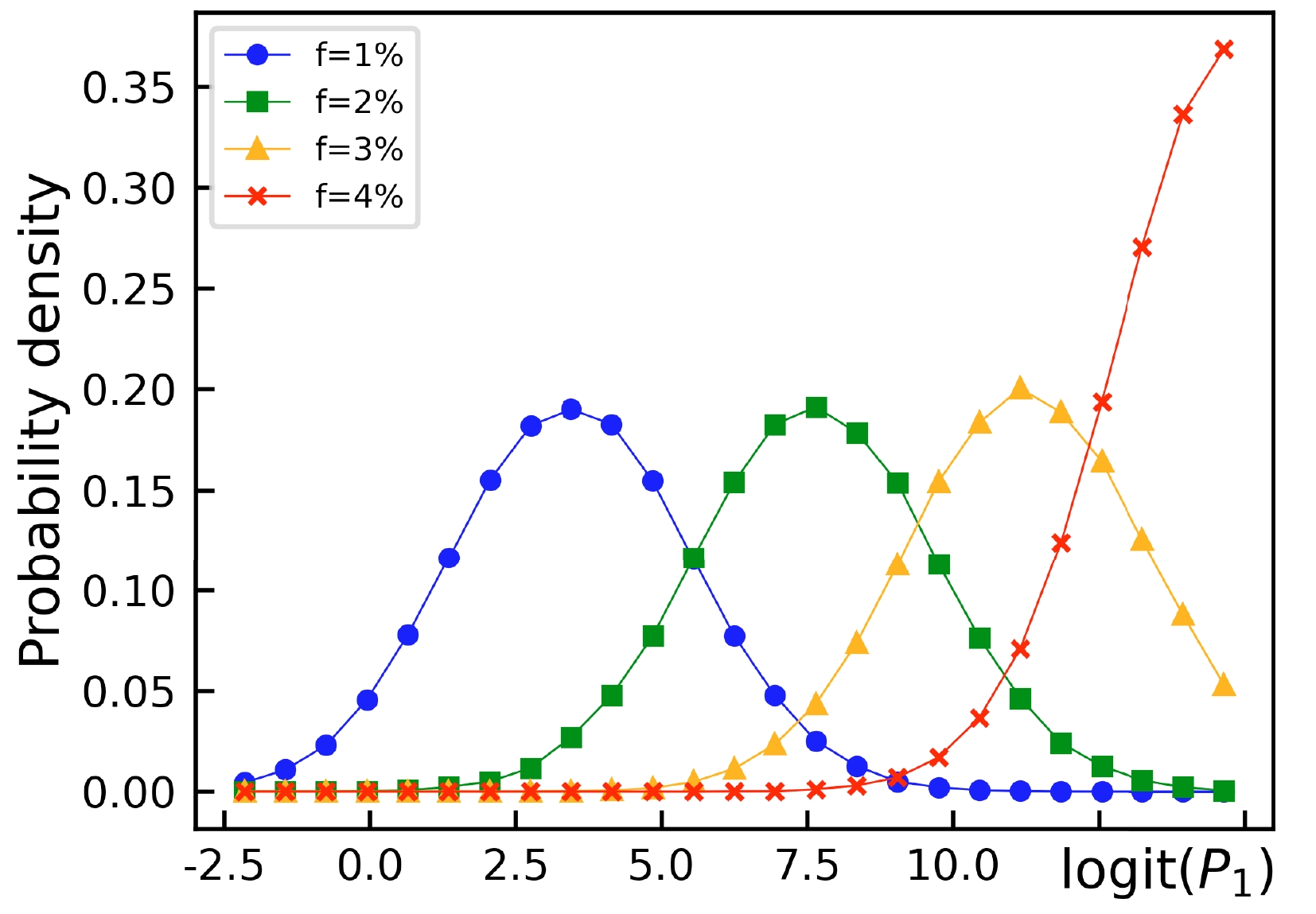
Figure 3. (color online) Distribution of logit(
$ P_1 $ ) on events @$ \sqrt{s_{NN}}=200 $ GeV and centrality 30%−40%. Tests were conducted on events with different initial charge quadrupoles ($ f=1\%-4\%$ ). The distributions are normalized to 1.The model was also validated through some other tests. In tests on no-CMW events generated by UrQMD, it classifies most events correctly as '0' class. To analyze whether the CME signal affects this CMW detector, a test set including AMPT events with CME was prepared. The trained model mostly output negative predictions.
Comparison with observables.— Above, we have demonstrated that the trained model efficiently decodes CMW information from
$ \rho^{\pm}(p_T, \phi) $ , providing a potential measure of CMW in heavy-ion collisions. However, further comparisons with experimental observables are necessary before constructing a measurement based on the model. Figure 3 shows that logit($ P_1 $ ) is correlated with f, which in turn has a positive correlation with the slope r. In addition to this slope, the following covariance between$ v_n $ and$ q_3 $ , which is essentially a three-particle correlator, constitutes another noteworthy observable [21],$ \lambda_n\equiv\langle v_n q_3\rangle - \langle q_3\rangle\langle v_n\rangle, $

(4) where
$ v_n $ is the n-th harmonic flow of the event,$ q_3 $ is the charge of the third particle, and$ \langle\cdots\rangle $ denotes event average. The differential three-particle correlator, which measures the correlation between the flow at a particular kinematic region and the charge of the third particle at another particular coordinate, is more convenient when comparing across experiments as no correction for efficiency is needed. In the following, we set$ n=2 $ for correlation with the elliptic flow. Using$ v_2^\mp\propto \bar{v}_2\pm r A_{\rm{ch}}/2 $ and$ A_{\rm{ch}}\sim\langle q_3\rangle $ , one notice that$ \lambda_2\approx\pm r(\langle A_{\rm{ch}}^2\rangle-\langle A_{\rm{ch}}\rangle^2)/2 $ for positive-charge/negative-charge cases. In the following,$ \lambda_2 $ is obtained by calculating half the difference between the positive-charge and negative-charge cases.Figure 4 shows the results of the comparison between logit(
$ P_1 $ ) and$ \lambda_2 $ . The average$ \lambda_2 $ of events increases gently as the response of the model becomes stronger. Knowing that logit($ P_1 $ ) is positively correlated to the CMW signal, this indicates a reasonable trend in$ \lambda_2 $ when the signal becomes stronger. This agrees with early studies on$ \lambda_2 $ [21] and also proves that the model prediction is qualified for measurement.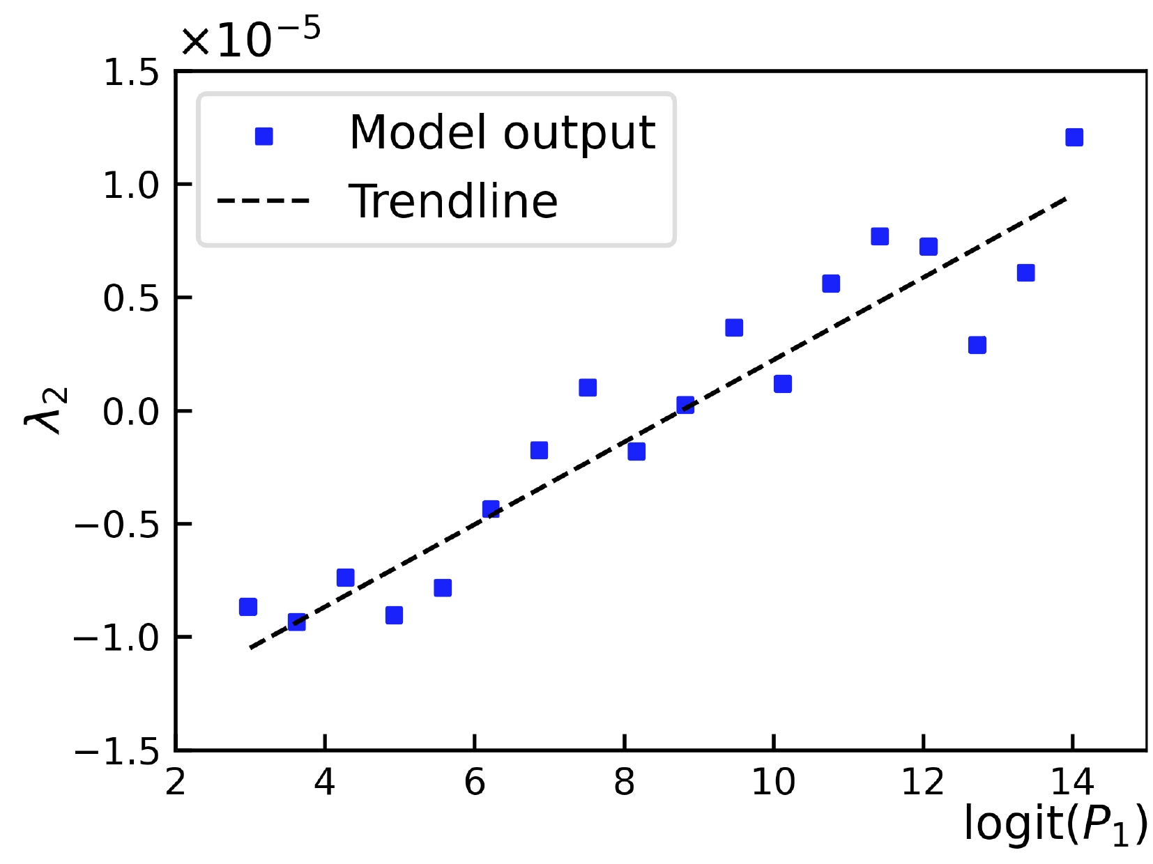
Figure 4. (color online) Distribution of logit(
$ P_1 $ ) on events for Au + Au at$ \sqrt{s_{NN}}=200 $ GeV and centrality 30%−40%. Events are divided into logit($ P_1 $ ) bins, and their$ \lambda_2 $ are averaged separately. The events are all embedded with the initial charge quadrupole. A range of logit($ P_1 $ ) was chosen in which most events are included, thereby avoiding statistical minority. The three-particle correlator clearly demonstrates a positive correlation with logit($ P_1 $ ).The performance under backgrounds must be evaluated before advancing. There are several mechanisms that may cause final-state
$ \Delta v_2 $ and$ A_{\rm{ch}} $ dependency, as discussed in Refs. [25–31]. To examine how the trained neural network performs under such backgrounds, its predictions for different$ \Delta v_2 $ ranges (either with or without initial charge quadrupoles) were analyzed. The results are shown in Fig. 5. For an input sample without CMW, the prediction increases when events with larger absolute$ \Delta v_2 $ are chosen. This shows that the neural network tends to regard events with larger$ \Delta v_2 $ as events containing CMW signals, although they do not actually include CMW signals. However, it should be emphasized that even in this situation,$ P_1 $ is still less than$ 0.5 $ , meaning that the neural network still correctly classifies them as events without CMW. For samples with CMW, the model exhibits strong robustness against the background, and the model classifies all the samples correctly.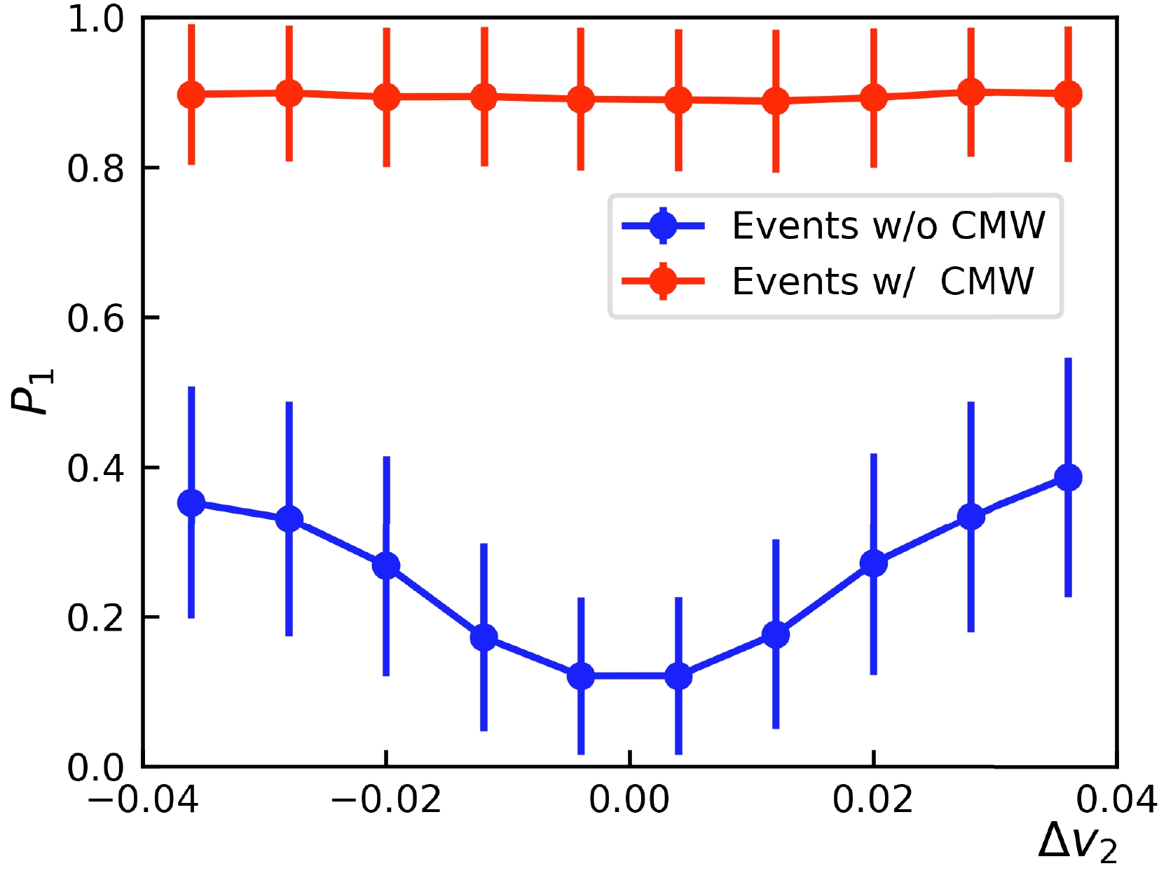
Figure 5. (color online) Distribution of
$ P_1 $ on events at$ \sqrt{s_{NN}}=200 $ GeV against$ \Delta v_2 $ . Events are divided into 10$ \Delta v_2 $ bins, and their$ P_1 $ values are averaged separately. As the magnitude of$ \Delta v_2 $ increases, the tendency of the model to output a false positive classification also increases. Nevertheless, in events involving an initial quadrupole, the model consistently maintains a high level of accuracy.Hypothesis test.— As previously discussed, the neural network demonstrates good accuracy in predicting the CMW signal and exhibits robustness across different collision energies, centralities, and background effects after training. This makes it feasible to create a CMW-meter based on this neural network. However, the need for averaging events poses a challenge when it comes to deploying this measurement experimentally, given that it is not possible to know the charge quadrupole pattern in advance or align events according to their charge distribution patterns.
However, from a hypothesis test perspective, the CMW-meter also holds experimental feasibility. For a fixed finite number M of events, one can assume the presence of a sufficiently large residual quadrupole that can be detected through our meter if CMW is assumed to exist in these events. Conversely, if no CMW is observed in experiments, the predictions output by the neural network will consistently fall within the '0' class. As demonstrated in Fig. 3, the intensity of the CMW signal significantly alters the distribution of logit
$ (P_1) $ or$ P_1 $ , thus influencing the distribution of$ P_1 $ itself (denoted by$ {\rm{P}}(P_1) $ ). This distribution responds differently depending on the presence or absence of CMW in the data set. If CMW exists in the heavy-ion collisions, the prediction of the neural network model regarding the residual quadrupole of a sample will align with$ {\rm{P}}(P_1) $ in the$ f \neq 0 $ case. In contrast, with no CMW signal, the distribution will match the$ f = 0 $ scenario. To establish a reasonable estimation of$ {\rm{P}}(P_1) $ for testing M events, we treat f as a latent variable representing CMW in a single event, as defined by the initial charge quadrupole fraction used in this study. For event-by-event fluctuations, we model f as a random variable following a Gaussian distribution,$ f \sim N(\mu, \sigma^2) $ , where μ is the mean of the latent variable f, which is expected to be around 0. The variance σ is estimated according to [37], where the average of$ |f| $ is approximately 2%,$ 2{\text{%}} =\langle\vert f\vert\rangle = \int\vert f\vert N^>(\vert f\vert;\sigma^2)\; {\rm d} \vert f\vert, $

(5) where
$ N^>(\vert f\vert;\sigma^2) $ is the half normal distribution and$ \vert f\vert $ is a positive-definite variable because the model prediction is independent of the sign of f. Solving Eq. (5) yields$ \sigma\simeq0.025 $ . Given that we employed averaged events to prepare the CMW-meter, the procedure to compose$ \rho(f_{\rm{eff}}) $ from single events$ \{\rho(f_i)\} $ becomes crucial, where$ f_{\rm{eff}} $ is the effective charge quadrupole rate of averaged events. One can choose the arithmetic mean as$ \frac{1}{M}\sum\limits_i^M \rho(f_i) = \rho\left(\frac{1}{M}\sum\limits_i^M f_i\right) = \rho(f_{\rm{eff}}). $

(6) Therefore, the distribution of
$ \vert f_{\rm{eff}}\vert $ can be achieved as$ F_{\rm{eff}}\sim N({\mu}/{M}, M\,{\sigma^2}/{M^2})=N(0, {\sigma^2}/{M}), $

(7) with
$ F_{\rm{eff}}\equiv\vert f_{\rm{eff}}\vert\sim N^>(\sigma^2/M) $ . The conditional probability$ {\rm{P}}(P_1\vert\;F_{\rm{eff}}) $ can be approximated as a Beta distribution,$ {\rm{Be}}(x;\alpha,\beta)=\frac{\Gamma(\alpha+\beta)}{\Gamma(\alpha)\Gamma(\beta)}x^{\alpha-1}(1-x)^{\beta-1}, $

(8) with α and β being the parameters of the Beta distribution, and Γ denoting the Gamma function. To describe
$ {\rm{P}}(P_1\vert\;F_{\rm{eff}}) $ at any$ F_{\rm{eff}} $ , we assume that α and β are functions of$ F_{\rm{eff}} $ and fit several sets of$ (\alpha, \beta) $ from the fitted beta distribution with a polynomial (for α) and Softplus (for β, to reach proper asymptotic behavior around$ {\rm{P}}_1=1 $ ).After parameterizing
$ {\rm{P}}(P_1\vert\;F_{\rm{eff}}) $ ,$ {\rm{P}}(P_1) $ is derived as$ \begin{aligned}[b] {\rm{P}}(P_1) &= \int{\rm{P}}(P_1\vert\,F_{\rm{eff}}){\rm{P}}(F_{\rm{eff}})\,{\rm d} F_{\rm{eff}}\\ &= \int_0^\infty{\rm{Be}}(P_1;\alpha(F_{\rm{eff}}), \beta(F_{\rm{eff}})) N^> \left(\frac{\sigma^2}{M}\right){\rm d} F_{\rm{eff}}. \end{aligned} $

(9) The numerical results are shown in Fig. 6.
$ {\rm{P}}(P_1) $ for the "existing CMW" has an evident rise around$ P_1=1 $ compared to the "no CMW" case, which suggests a non-zero probability of composing a large residual quadrupole. With a smaller M, the width of$ f_{\rm{eff}} $ becomes larger, which allows obtaining a visible$ P_1 $ . Figure 6 also presents results of random mixing events of both charge quadrupole patterns generated by AMPT, where$ M= $ 25. For both large- and small-$ {\rm{P}}_1 $ areas, these results are qualitatively consistent with our hypothesis test analysis, which indicates that the trained neural network is capable of recognizing charge quadrupoles with less averaged events.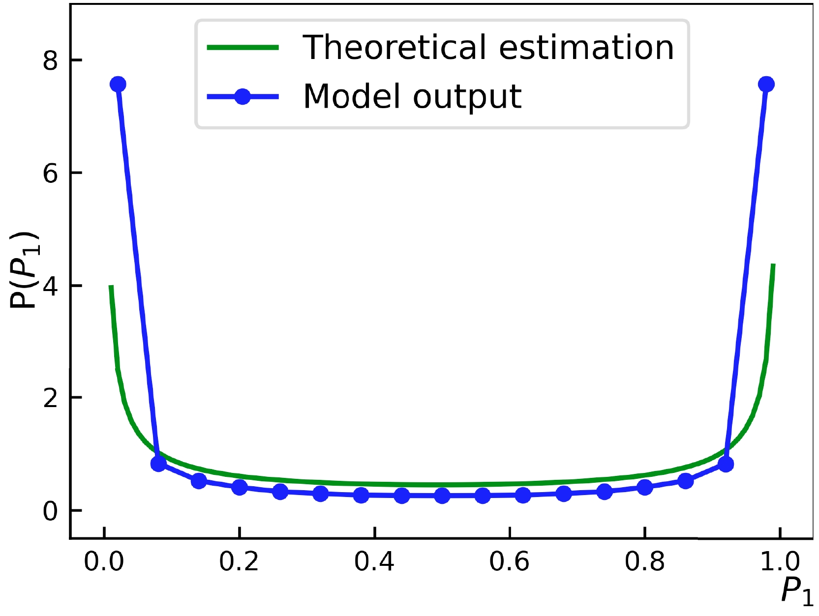
Figure 6. (color online)
$ {\rm{P}}(P_1) $ for AMPT events with$ M=25 $ . The peak of this distribution near$ P_1=0 $ suggests that the charge quadrupole in most events negate each other, and the peak near$ P_1=1 $ is due to the strong response to some large enough residual quadrupole. -
In this paper, we propose a deep convolutional neural network model for CMW detection. Building upon a previous study of ours [38] focused on deep-learning-based CME detection, this model expands its application to CMW detection. We trained the neural network using data generated from the AMPT model for Au + Au collisions at 200 GeV, with the CMW-like initial charge quadrupole encoded. The trained model exhibits a robust capability to discern events with CMW from those without, and it can quantitatively measure the fraction or strength of the initial charge quadrupole, effectively functioning as a CMW-meter. Furthermore, we validated the model's performance across a broad range of collision energies and centralities, thereby demonstrating its resilience. We also checked that the trained model is well qualified even for other collision systems such as Zr + Zr and Ru + Ru collisions. Comparative analysis against three-particle correlators and
$ \Delta v_2 $ proves the model's effectiveness even in the presence of strong backgrounds. By employing a hypothesis test, an experimentally viable analysis based on the model can be established, wherein the distribution of model predictions serves as an indicator of CMW occurrence in the data.One drawback of the proposed model is that its brightness is achieved at the cost of generalization ability, as the training data is confined to a narrow range of collision energies. In the future, it would be interesting to enhance the generalization capabilities of the model and transform it into an end-to-end CMW meter.
-
We acknowledge the useful discussions with L.-X. Wang and K. Zhou.
Applying deep learning technique to chiral magnetic wave search
- Received Date: 2024-03-03
- Available Online: 2024-08-15
Abstract: The chiral magnetic wave (CMW) is a collective mode in quark-gluon plasma originated from the chiral magnetic effect (CME) and chiral separation effect. Its detection in heavy-ion collisions is challenging owing to significant background contamination. In [Y. S. Zhao et al., Phys. Rev. C 106, L051901 (2022)], we constructed a neural network that accurately identifies the CME-related signal from the final-state pion spectra. In this study, we have generalized this neural network to the case of CMW search. We show that, after an updated training, the neural network effectively recognizes the CMW-related signal. Additionally, we have assessed the performance of the neural network in comparison with other known methods for CMW search.


 DownLoad: