


 Abstract
 HTML
HTML Reference
 Related
 PDF
PDF


-
A black hole is an extreme celestial body predicted by the general relativity [1]. Inspired by the presentation of the Bekenstein's entropy [2] for the black hole, Hawking concluded that when the quantum effect is taken into account, a black hole emits thermal radiation just like a normal black body. This means that the black hole has a temperature. The concept that black holes possess entropy and temperature is undoubtedly one of the most important discoveries of the 20th century and has been a topic of discussion for decades.
A central element of black hole thermodynamics is the phase transition, i.e., the transition from one state to another, accompanied by abrupt changes in physical quantities such as energy, entropy, and volume under different parameter conditions. Hawking and Page first investigated the thermodynamic properties of the Anti-de Sitter (AdS) black hole and found that there is a phase transition between the Schwarzschild AdS black hole and pure AdS thermal radiation, i.e., the famous Hawking-Page phase transition [3]. Subsequently, the black hole thermodynamics ushered in groundbreaking achievements under the pioneering work [4]. The extended phase space of the AdS black hole thermodynamics was introduced, where the negative cosmological constant is considered as the effective thermodynamic pressure of the black hole and its conjugate quantity is the thermodynamic volume, which initiated the recent surge of interest in the extended black hole thermodynamics. The small-large black hole phase transition presented by the charged AdS black hole thermodynamic system has a more direct and precise overlap with the van der Waals system [5−11]. Currently, the study of the phase transition of black holes in the extended phase space has been widely applied to various complex scenarios [12−17].
In addition, the holographic thermodynamics [18−21] and restricted phase space thermodynamics [22−25] have been proposed to give a holographic interpretation of the black hole thermodynamics and to make it more like ordinary thermodynamics. Moreover, the topology has emerged as a new way to describe the type of the phase transition in black holes. In a study [26, 27], it is described in detail how to use the
$ \phi $ -map topological flow theory to construct a topological number that is independent of the endogenous parameters of black holes. The topological number can be used to distinguish between locally stable and locally unstable black hole phases as well as to topologically classify the same class of black holes [28−32]. These studies can deepen our understanding of black hole physics and contribute to the search of clues to reveal the nature of black holes and quantum theory of gravity.The analysis of the type and criticality of the thermodynamic phase transition in black holes currently dominates the investigations. The swallowtail diagrams of the Gibbs free energy can provide certain answers about the macroscopic thermodynamic processes of the black hole phase transitions, but they overlook the details of the phase transitions. Some ideas have been proposed to use the free energy landscape [33−35] and Landau free energy [36] to explore the evolutionary processes associated with the black hole phase transitions.
In a recent study [37], the author constructed a thermal potential to study the black hole phase transition. The thermal potential or generalized free energy is
$ U=\int(T_h-T){\rm d}S, $

(1) where
$ T_h $ is the Hawking temperature of the black hole, T is the canonical ensemble temperature, and S is the entropy of the black hole. Parameters U,$ T_h $ , and S are the functions of radius of the event horizon$ r_h $ , and T is just a positive constant, which can be assigned in any way. When a standard system is determined to be a black hole, the ensemble temperature of the system should be the Hawking temperature of the black hole, i.e.,$ T=T_h $ . Similar to the fluctuation, the thermal potential shows that all other possible thermodynamic states of the system deviate from the black hole states. The above thermal potential or generalized free energy is a undefinite integration. Here, we assume the integration constant to be zero. If it is non-zero, we absorb it into U without changing the qualitative results in the present paper. We are currently conducting a comprehensive analysis of phase transitions, only extracting the qualitative behavior of phase transitions and not strictly requiring quantitative results.From Eq. (1), it follows that the extremum of the potential represents all possible black hole states,
$ \dfrac{{\rm d}U}{{\rm d}S}=0\; \; \Rightarrow\; \; T=T_h. $

(2) More importantly, the concave (convex) nature of the thermal potential represents the stable (unstable) state of the black hole,
$ \delta \Biggl( \dfrac{{\rm d}U}{{\rm d}S}\bigg|_{T=T_h} \Biggr)=\left\{ \begin{array}{*{20}{ll}} \dfrac{\partial T_h(r_h)}{\partial S(r_h)}\bigg|_{T=T_h}>0,&{\rm{stable \; case}};\\ \dfrac{\partial T_h(r_h)}{\partial S(r_h)}\bigg|_{T=T_h}<0,&{\rm{unstable \; case}}. \end{array} \right. $

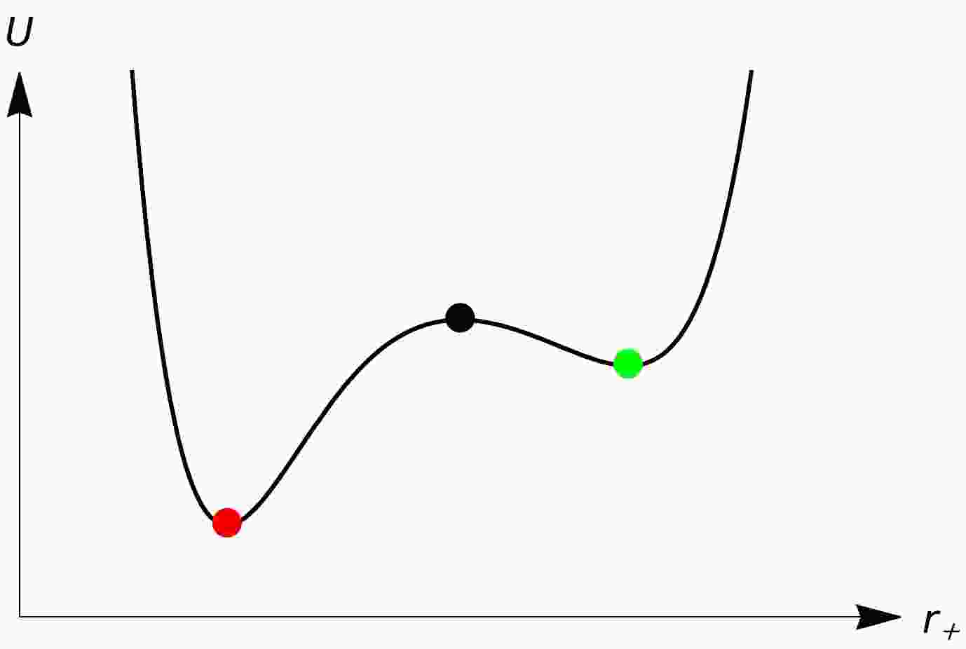
(3) A diagram of thermal potential described by Eq. (1) is shown in Fig. 1. It is certain that the lowest point (the red point) is the most stable state in the entire canonical ensemble. As the different parameters of the black hole change, the extreme point of the thermal potential constantly changes, which corresponds to the changes between the black hole state and other unknown states in the ensemble. In the framework, we studied the microscopic phase transition mechanism of the charged AdS black holes [38] and found that the phase transition of large and small black holes exhibits severely asymmetric features, which fills the gap in the analysis of stochastic processes in the first-order phase transition rate problem of AdS black holes.
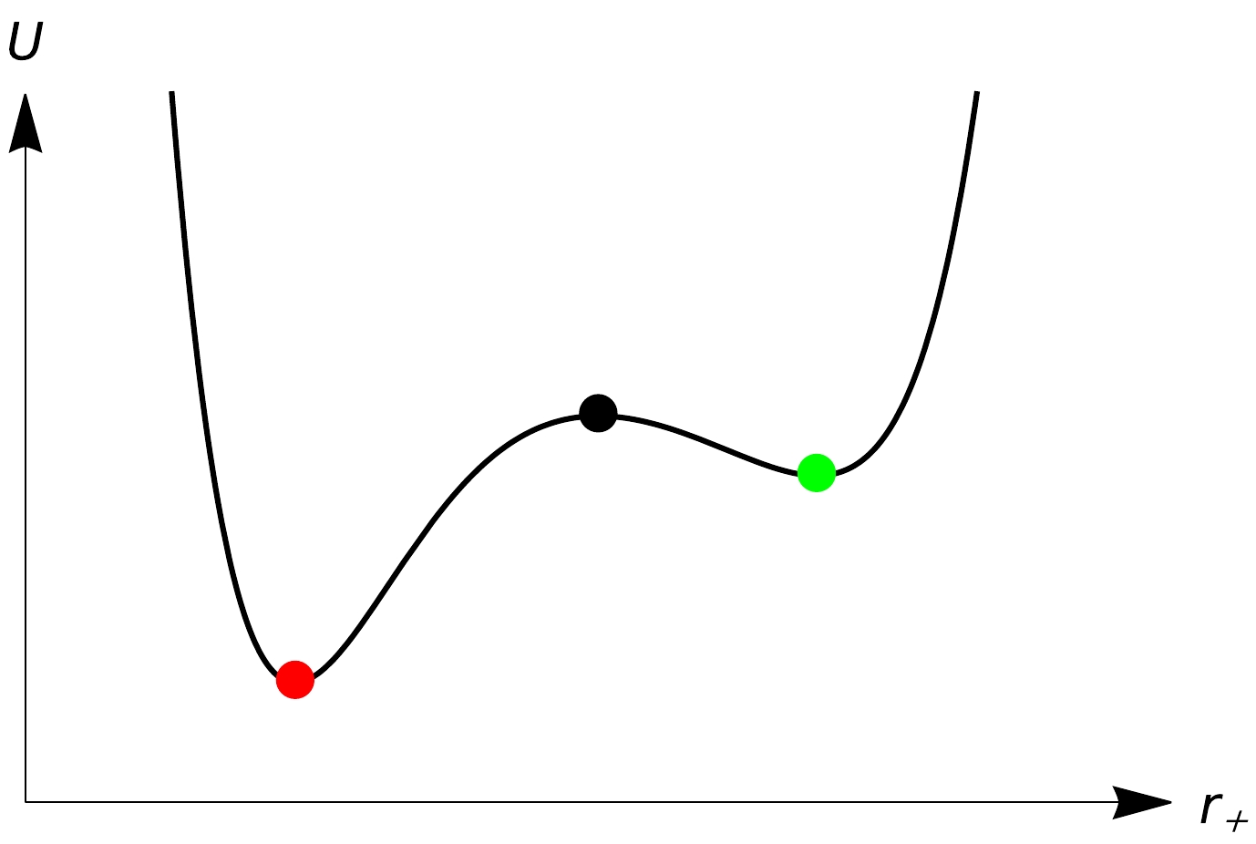
Figure 1. (color online) Diagram of thermal potential, where
$\color{red}{\bullet} $ represents the global minimum,$\bullet $ represents the local maximum, and$\color{green}{\bullet} $ represents the local minimum.In the four-dimensional spacetime, Einstein gravity can give the most appropriate explanation. While in higher dimensions, when the energy approaches the Planck energy scale, the high-order curvature terms of spacetime cannot be neglected, and Einstein's general relativity theory requires some modifications. One of the widely accepted and valid candidates is the Lovelock gravity. Naturally, Lovelock gravity is an extension of Einstein gravity in a higher dimensional spacetime, and it proposes that the quantities acting in higher dimensional gravity should contain high-order gauge terms. The black hole solution in this gravity and the associated thermodynamic properties have been extensively studied [39−43]. When we consider the third-order Lovelock gravity, its action contains four terms: the cosmological constant term, Einstein action term, Gauss-Bonnet term, and third-order Lovelock term. The black hole thermodynamics under third-order Lovelock gravity has also been widely studied [44−48]. Thus, the specific details behind its phase transition become the main object to study. This inspires us to explore and analyze the microscopic processes of the phase transition of small and large black holes in third-order Lovelock black holes. Through the thermal potential and complex analysis, we study how a black hole transforms from one black hole state to another under the influence of temperature T and pressure P in order to obtain its specific transition processes. We wish to further enrich the black hole phase transition dynamics process.
The structure of this paper is as follows: In Sec. II, we present a brief introduction to third-order Lovelock black holes. Then, the winding number is related to black hole thermodynamics using the complex analysis approach. In Sec. III, the phase transition in the hyperbolic case is studied, focusing on
$ d = 7 $ . In Sec. IV, the phase transition in the spherical case is further studied, focusing on the analysis of$ d = 7 $ and$ d = 9 $ cases. Finally, Sec. V is devoted to a summary and discussion. -
First, the d-dimensional Lovelock Lagrangian density is [39, 49, 50]
$ {\cal{L}}=\sum\limits_{n=0}^N \alpha_n \lambda^{2(n-1)} {\cal{L}}_n, $

(4) $ {\cal{L}}_n=\frac{1}{2^n} \sqrt{-g} \delta_{j_1 \ldots j_{2 n}}^{i_1 \ldots i_{2 n}} R_{i_1 i_2}^{j_1 j_2} \ldots R_{i_{2 n-1} i_{2 n}}^{j_{2 n-1} j_{2 n}}, $

(5) where
$ N=\left\{ \begin{array}{*{20}{ll}} \dfrac{d}{2}-1,&\; \; \; \; {\rm{for \; even }}\; d,\\ \dfrac{d-1}{2},&\; \; \; \; {\rm{for\; odd}}\; d, \end{array} \right.\\ $

(6) and n is the order,
$ \alpha_n $ and$ \lambda $ are the coupling constants for each of the Lagrangian density functions, g is the determinant of metric$ g_{\mu\nu} $ ,$ R^{\lambda}{}_{\mu \nu \rho} $ is the Riemann tensor,$R^{\lambda\mu}{}_{ \nu \rho}= g^{\mu \beta}R^{\lambda}{}_{\beta \nu \rho}$ , and$ \delta_{j_1 \ldots j_{2 n}}^{i_1 \ldots i_{2 n}} $ is the generalized Kronecker delta of order$ 2n $ . For the calculation, here, we list the first four items of the Lagrangian:$ {\cal{L}}_0= \sqrt{-g}, $

(7) $ {\cal{L}}_1= \frac{1}{2} \sqrt{-g} \delta_{j_1 j_2}^{i_1 i_2} R_{i_1 i_2}^{j_1 j_2}=\sqrt{-g} R, $

(8) $ \begin{aligned}[b] {\cal{L}}_2=\;& \frac{1}{4} \sqrt{-g} \delta_{j_1 j_2 j_3 j_4}^{i_1 i_2 i_3 i_4} R_{i_1 i_2}^{j_1 j_2} R_{i_3 i_4}^{j_3 j_4} \\ =\;&\sqrt{-g}\left(R_{\mu \nu \rho \sigma} R^{\mu \nu \rho \sigma}-4 R_{\mu \nu} R^{\mu \nu}+R^2\right), \end{aligned} $

(9) $ \begin{aligned}[b] {{\cal{L}}_3} =\; & \frac{1}{8} \sqrt{-g} \delta_{j_1 j_2 j_3 j_4 j_5 j_6}^{i_1 i_2 i_3 i_4 i_5 i_6} R_{i_1 i_2}^{j_1 j_2} R_{i_3 i_4}^{j_3 j_4} R_{i_5 i_6}^{j_5 j_6} \\ =\; & \sqrt{-g} (R^3 +2 R^{\mu \nu \sigma \kappa} R_{\sigma \kappa \rho \tau} R_{\mu \nu}^{\rho \tau}+8 R_{\sigma \rho}^{\mu \nu} R_{\nu \tau}^{\sigma \kappa} R^{\rho \tau} \end{aligned} $

$ \begin{aligned}[b]&+24 R^{\mu \nu \sigma \kappa} R_{\sigma \kappa \nu \rho} R_{\mu}^\rho +3 R R^{\mu \nu \sigma \kappa} R_{\mu \nu \sigma \kappa} \\&+24 R^{\mu \nu \sigma \kappa} R_{\sigma \mu} R_{0\kappa \nu}+16 R^{\mu \nu} R_{\nu \sigma} R_\mu^\sigma-12 R R^{\mu \nu} R_{\mu \nu}). \end{aligned} $

(10) From Eqs. (4) and (6), it is known that n-order Lagrangian
$ {\cal{L}} $ depends on different dimensions d.● When
$ d=4 $ , order n is 1. The 1-order Lagrangian contains$ {\cal{L}}_0 $ and$ {\cal{L}}_1 $ , and it is also called the Einstein-Hilbert Lagrangian in 4 dimensions ($ {\cal{L}}_0 $ and$ {\cal{L}}_1 $ are the cosmological constant term and Einstein term, respectively).● When
$d=5 $ and$d=6 $ , order n is 2. The 2-order Lagrangian includes$ {\cal{L}}_0 $ ,$ {\cal{L}}_1 $ , and$ {\cal{L}}_2 $ , and it is also called the Einstein-Gauss-Bonnet Lagrangian ($ {\cal{L}}_2 $ is the Gauss-Bonnet term) [51, 52].● By analogy, for n = 3, the 3-order Lovelock Lagrangian contains
$ {\cal{L}}_0 $ ,$ {\cal{L}}_1 $ ,$ {\cal{L}}_2 $ , and$ {\cal{L}}_3 $ , and it exists in 7 and 8 dimensions ($ {\cal{L}}_3 $ is the third-order Lovelock term).● The contribution of higher-order Lovelock terms becomes smaller gradually to the point where it can be ignored. Hence, the
$ n (n \ge 4) $ -order Lagrangian can be approximated as the one with the order of 3, and then the 3-order Lovelock theory is used to study black holes in$ d\geq 7 $ dimensions naturally.Hence, the geometric action of the third-order Lovelock black hole is written as [47, 48]
$ \begin{aligned}[b] {\cal{I}} =\;&\dfrac{1}{16\pi G}\int d^dx \left(\dfrac{\alpha_0}{\lambda^2}{\cal{L}}_0 +\alpha_1{\cal{L}}_1+\alpha_2\lambda^2{\cal{L}}_2+\alpha_3\lambda^4{\cal{L}}_3\right) \\=\;&\dfrac{1}{16\pi G}\int d^dx(R-2\Lambda+\hat\alpha_2{\cal{L}}_2+\hat\alpha_3{\cal{L}}_3), \end{aligned} $

(11) and we have taken the liberty of making
$ \alpha_0=-2\Lambda \lambda^2, \alpha_1=1, ~ \hat\alpha_2=\alpha_2\lambda^2 $ , and$ \hat\alpha_3=\alpha_3\lambda^3 $ . In the following formulation, we choose$ \alpha $ instead of$ \hat\alpha_2 $ and$ \hat\alpha_3 $ ,$ \hat\alpha_{2}=\frac{\alpha}{(d-3)(d-4)}, \quad \hat\alpha_{3}=\frac{\alpha^2}{72{d-3\choose 4}}. $

(12) The static spherical symmetry metric for
$ d \ge 7 $ is expressed as [39−41]$ {\rm d}s^2=-V(r){\rm d}t^2+\dfrac{1}{V(r)}{\rm d}r^2+r^2{\rm d}\Omega_k^2, $

(13) $ V(r)=k+\dfrac{r^2}{\alpha}\Bigg[1-\Bigl(1+\dfrac{6\Lambda \alpha}{(d-1)(d-2)}+\dfrac{3\alpha m}{r^{d-1}}\Bigr)^{\frac{1}{3}}\Bigg], $

(14) where m is a parameter related to the mass of a black hole, and k is the topology of the spacetime curvature and can take –1, 0, and 1.
The Hawking temperature of the third-order black hole in terms of the radius of the event horizon
$ r_h $ is$ \begin{aligned}[b]T_h=\;&\dfrac{1}{12\pi r_h(r_h^2+k\alpha)^2}\Bigg[\dfrac{48\pi P r_h^6}{(d-2)}+3(d-3)kr_h^4\\&+3(d-5)\alpha k^2r_h^2+(d-7)\alpha ^2k\Bigg], \end{aligned} $

(15) where P is the pressure via
$ P=-\Lambda/(8\pi G) $ . Usually, the black hole entropy satisfies the area formula, i.e., the black hole entropy is equal to one quarter of the event horizon area. However, in higher derivative gravity, the area law of entropy is not satisfied in general. The thermodynamic method is the simplest way to obtain the entropy of the higher derivative gravity. Indeed, we can also obtain the entropy from the Wald's Noether charge technique [53, 54]. Here, we derive the expression for the entropy of a black hole from a thermodynamic perspective [55].Black hole mass M, temperature T, and entropy S satisfy the first law of thermodynamics dM=TdS, where mass M per unit volume
$ \Sigma_k $ can be expressed as$ (d-2)m/(16\pi G) $ , and$ \Sigma_k $ represents the volume of the$ (d-2) $ -dimensional submanifold,$ M=\dfrac{(d-2) m}{16\pi G}=\dfrac{(d-2) r_h^{d-3}}{16\pi}\bigg(k+\dfrac{16\pi Pr_h^2}{(d-1)(d-2)}+\dfrac{\alpha k}{r_h^2}+\dfrac{\alpha^2k}{3r_h^4}\bigg). $

(16) Integrating the first law and starting the horizon radius from zero, we can obtain entropy per unit volume
$ \Sigma_k $ conjugated to the temperature [55] as$ S=\int_{0}^{r_h}T_h^{-1}\dfrac{\partial M}{\partial r_h} {\rm d} r_h=\dfrac{r_h^{d-2}}{4}\left[1+\dfrac{2(d-2)k\alpha}{(d-4)r_h^2}+\dfrac{(d-2)k^2\alpha^2}{(d-6)r_h^4}\right]. $

(17) The entropy is not only one quarter of the surface area of the horizon but also reproduces the expression for the entropy of Lovelock black holes derived by Hamiltonian methods in [56, 57], which state that the entropy includes a sum of intrinsic curvature invariants integrated over a cross section of the horizon.
In thermodynamics, we know that entropy and mass are extensive variables, whereas temperature is an intensive variable. Here, we introduce mass M per unit volume
$ \Sigma_k $ and entropy per unit volume$ \Sigma_k $ to analyze the thermodynamic properties of black holes. The overall thermodynamic properties of the system can be replaced by the thermodynamic properties per unit volume to obtain the qualitative characteristics of the thermodynamic system of a black hole. This avoids the uncertainty of volume of the sub-manifold$ \Sigma_k $ in the hyperbolic case.Therefore, thermal potential per unit volume
$ \Sigma_k $ of the third-order Lovelock black hole is expressed as$ \begin{aligned}[b] U=\;&\int(T_h-T){\rm d}S=\dfrac{r_h^{d-7}}{48 \pi (d-1)}\Bigg[48 \pi P r_h^6\\&+(d-1)(d-2)\Big(3kr_h^4+3\alpha k^2r_h^2+\alpha^2k\Big)\Bigg]\\ &{-\dfrac{T r^{d-2} }{4} \bigg[1+\dfrac{2(d-2)k\alpha}{(d-4)r_h^2}+\dfrac{(d-2)k^2\alpha^2}{(d-6)r_h^4}\bigg].} \end{aligned} $

(18) According to Eqs. (1) and (2), we define function
$ f(r_h) $ as the first derivative of the generalized free energy with respect to the horizon radius,$ f(r_h)=\dfrac{{\rm d} U(r_h)}{{\rm d} S(r_h)}. $

(19) At this point, the information of the black hole thermodynamic system is reflected by the characteristics of zeroes of function
$ f(r_h) $ because if$ f(r_h)=0 $ , we obtain$ T=T_h $ . The different states of a black hole thermodynamic system are at the extreme points of the generalized free energy. Thus, we can turn the thermodynamic problems into solving the zeroes of real function$ f(r_h) $ . To see the full picture of the problem, we need to change real function$ f(r_h) $ to complex continuation function$ f(z) $ , and use the method of complex analysis [58].In complex analysis, the Argument Principle is an effective method to calculate the number of zeros of analytic functions. If
$ f(z) $ is a meromorphic function in simple closed contour C and is analytically nonzero on C, then$ N(f, C)-P(f, C)=\frac{1}{2 \pi {\rm i}} \oint_C \frac{f^{\prime}(z)}{f(z)} {\rm{d}} z=\frac{\Delta_C \arg f(z)}{2 \pi}, $

(20) where
$ N(f, C) $ and$ P(f, C) $ are respectively the number of zeros and poles of$ f(z) $ in C,$ f'(z) $ is the first order derivative of$ f(z) $ , and$ \text{arg}f(z) $ is the argument of$ f(z) $ . Making transformation$ \omega = f(z) $ , the above equation is then expressed as the number of rotations of$ \omega $ around the origin of curve$C' $ as complex variable z moves around complex envelope C, where$C' $ is the image curve of C after the transformation. The winding number is denoted by$ W:=\frac{1}{2 \pi {\rm i}} \oint_{C'} \frac{{\rm{d}} \omega}{\omega}=\frac{1}{2 \pi {\rm i}} \oint_C \frac{f^{\prime}(z)}{f(z)} {\rm{d}} z. $

(21) If analytic function
$ f(z) $ does not have poles within the complex perimeter, the winding number of the origin is$ W=N(f, C) $ . When complex variable z varies on contour C, the image of argument function$ \theta = \text{arg}f(z) $ can be a Riemann surface. The winding number of the origin corresponds to the foliations of the Riemann surface of the complex variable function.In [58], we have preliminarily summarized an empirical correspondence through several typical thermodynamic systems of black holes (Schwarzschild, Schwarzschild AdS, Reissner-Nordström, charged AdS, and 6-dimensional charged Gauss-Bonnet black holes), that is, the correspondence between winding number W and the phase transition of black holes. Specifically, when
$W=1 $ , there is no phase transition; when$W=2 $ , it corresponds to the second-order phase transition; and when$W=3 $ , it means that the first-order phase transition will occur, accompanied by the second-order phase transition. Through this empirical conclusion, we can predict the phase transition characteristics of other black hole thermodynamic systems.Here, we consider only zeros that are real and positive, and these correspond to physical values for radius
$ r_h $ . Next, we expect to use this method to predict the structure of the phase transitions of the third-order Lovelock black hole. In planar topology$k=0 $ , the temperature of the black hole can be expressed as$ T_h=4Pr_h/(d-2) $ , resulting in the equation of state$ P=T_h/v $ with$v=4r_h/ (d-2)$ . It is the same as that of an ideal gas. There are no phase transitions in the planar topology for any dimensions. Therefore, we will focus on two cases$ k = -1 $ and$ k = +1 $ . -
In this case, we have
$k=-1 $ . For the Lovelock black hole in the hyperbolic case, analytic function$ f(z) $ is calculated by Eqs. (18) and (19) as follows:$ \begin{aligned}[b] f(z)=\;&\dfrac{1}{12\pi z(z^2-\alpha)^2}\Bigg[\dfrac{48\pi P z^6}{(d-2)}-3(d-3)z^4\\&+3(d-5)\alpha z^2-(d-7)\alpha ^2-12\pi z T(z^2-\alpha)^2\Bigg]. \end{aligned} $

(22) Whether
$d=7 $ or$ 7<d\le 12 $ , this analytic function has three zeros at most in the entire complex plane$ {\bf{C}} $ with the singularities removed. The only difference between them is that the singularities are$ \pm\sqrt{\alpha} $ for$d=7 $ , whereas for$ 7<d\le 12 $ , the singularities are 0 and$ \pm\sqrt{\alpha} $ . Hence, we obtain winding number$W=3 $ and its complex structure is the Riemann surface with three foliations, as shown in Fig. 2. Based on the results of the study [58], we predict that the black hole will undergo the phase transitions with the first and second orders.
Figure 2. (color online) Riemann surface of the first-order and second-order phase transitions for the black hole system.
Since
$d=7 $ is of the same type as$ d > 7 $ , let us make a long story short and use$d=7 $ as an example to verify the above viewpoint. We know that there is only one set of critical points in the hyperbolic case, and we obtain the critical points for$d=7 $ from [47, 48]$ P_c=\dfrac{5}{8\pi \alpha},\qquad T_c=\dfrac{1}{2\pi \sqrt{\alpha}},\qquad v_c=\dfrac{4}{5}\sqrt{\alpha}. $

(23) For the sake of discussion, we introduce the following dimensionless thermodynamic quantities:
$ \begin{aligned}[b]& p:=\dfrac{P}{P_c},\qquad t:=\dfrac{T}{T_c},\qquad x:=\dfrac{r_h}{r_c},\\& t_h:=\dfrac{T_h}{T_c},\qquad s:=\dfrac{S}{S_c},\qquad u:=\dfrac{U}{|U_c|}. \end{aligned} $

(24) The validity of the method is now checked with an analysis of the behavior of the thermal potential. After a series of calculations, we obtain the dimensionless thermal potential for d = 7,
$ u=\dfrac{5}{16}(px^6-3x^4+3x^2-1)-\dfrac{3}{8}t \left(x^5-\dfrac{10}{3}x^3+5x \right). $

(25) From Eq. (25), it can be observed that the two key parameters (p and t) affect the behavior of the thermal potential. Here, we fix parameter t to observe the variation of the thermal potential with p. In Fig. 3, we show the
$ u-x $ plot at$d = 7 $ . According to Eqs. (1) and (3), we know that the black hole state can be placed at an extreme value of the thermal potential. An unstable black hole state is at the local maximum point, and a stable black hole state is at the minimal point. The lower the potential, the higher the probability that the black hole is at that point and the more stable is the system.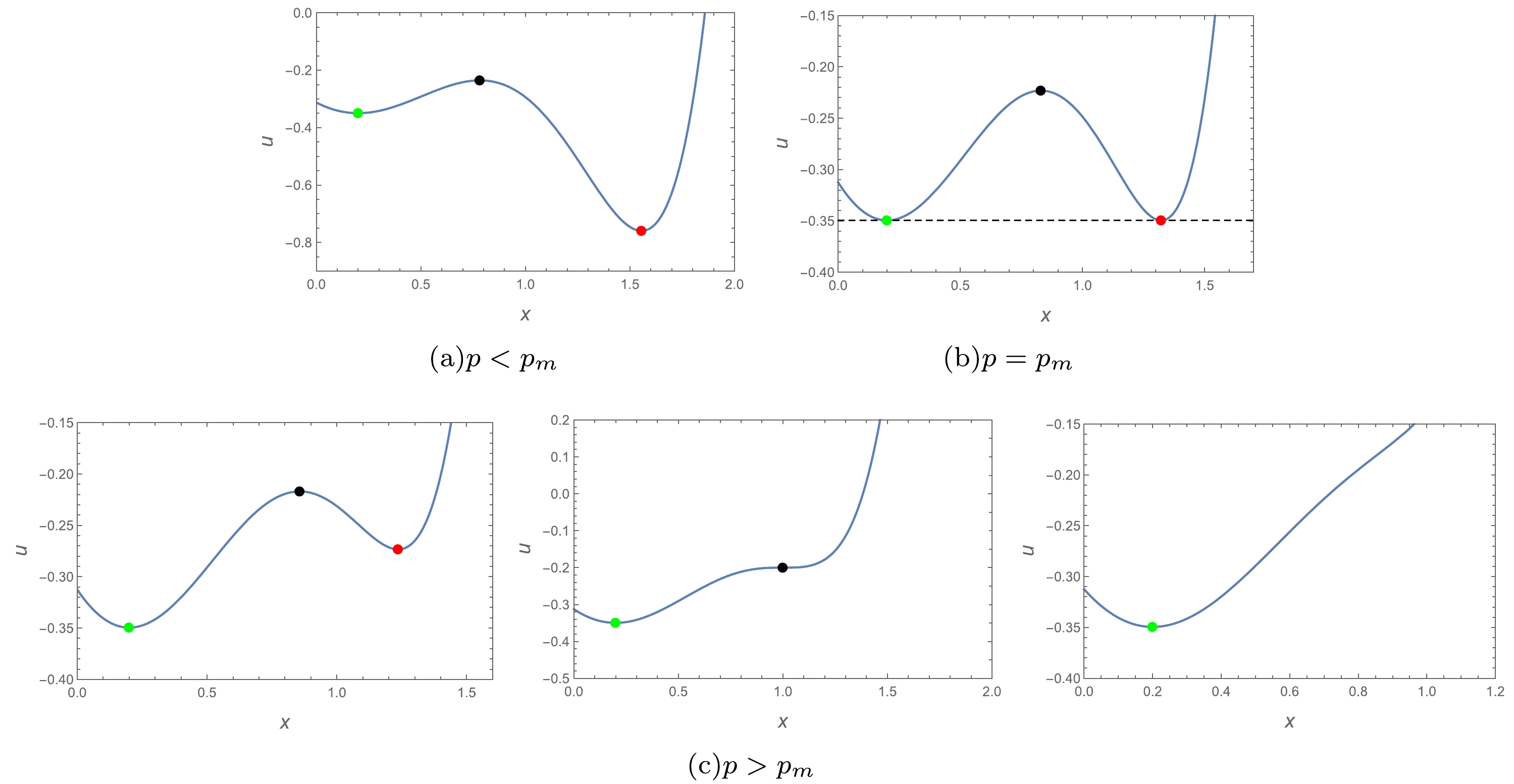
Figure 3. (color online) u-x plots of
$t=0.2 $ for$d = 7 $ . The$\color{green}{\bullet} $ -phase in the diagram represents the small black hole state,$ \color{red}{\bullet} $ -phase represents the large black hole state, and$ {\bullet} $ -phase represents the unstable black hole state. Pressure p increases from left to right in the$ p > p_m $ plots.From diagrams (a) and (b) in Fig. 3, we find that at fixed temperature
$t=0.2 $ (for any value$ 0 < t < 1 $ , we always obtain the same result), a global minimum and local minimum start to change as pressure p increases from$p=0 $ to$ p=p_m $ , at which point the global minima of the thermal potential are equivalent. Specifically, at$ 0 < p < p_m $ , the thermal potential of the large black hole phase is lower than that of the small black hole phase, implying that the system tends toward the large black hole phase. When p increases to$ p_m $ , the large and small black hole phases are in equilibrium. Similarly, it is clear from diagrams (b) and (c) that as p increases, the two equivalent global minima begin to change. The small black hole phase is at the global minimum, whereas the large black hole phase changes to be in the local minimum until it disappears. Specifically, the thermal potential of the small black hole phase is lower than that of the large black hole phase, which means that the system tends toward the small black hole phase at$ p > p_m $ .Thus, it is clear from the above analysis that in the
$ k=-1 $ hyperbolic case, the system has a first-order phase transition from a large to small black hole. From Eq. (23), it follows that there is a critical point, which is the inflection point of the curve; therefore, the system also has a second-order phase transition. This is exactly what we predicted. -
In this case, we have
$ k=+1 $ . For the Lovelock black hole in the spherical case, the analytic function is calculated by Eqs. (18) and (19),$ \begin{aligned}[b] f(z)=\;&\dfrac{1}{12\pi z(z^2+\alpha)^2}\Bigg[\dfrac{48\pi P z^6}{(d-2)}+3(d-3)z^4+3(d-5)\alpha z^2\\&+(d-7)\alpha ^2-12\pi z T(z^2+\alpha)^2\Bigg].\\[-10pt]\end{aligned} $

(26) Here, we note that the zeroes of the cases in
$d = 7 $ and$d > 7 $ are not equal across the complex plane with all singularities removed, which leads to different winding number and Riemann surfaces. Thus, the spherical case is not as straightforward as the hyperbolic one and needs to be discussed differently.In particular, at
$d=12 $ , there is only one zero point; thus, the winding number is 1 and it is a single-foliation Riemann surface. As a result, the system does not undergo a phase transition. This conclusion is already well-known and is not elaborated here. -
For
$d=7 $ , we can obtain its analytic function from Eq. (26) as$ f(z)=\dfrac{1}{10\pi (z^2+\alpha)^2}\bigg[(8P\pi z^5+10z^3+5\alpha z)-10\pi T (z^2+\alpha)^2\bigg]. $

(27) Similarly, there are three zeroes at most on complex plane
${\bf{C}}\backslash \{ \pm \sqrt{\alpha} {\rm i}\}$ , so that winding number$W=3 $ and the complex structure is similar to the hyperbolic case in$d=7 $ with three foliations. Hence, we predict that the second-order and first-order phase transitions will occur. Next, we verify its correctness by the thermal potential.First, from [48], we obtain critical points
$ P_{c1}=0,\qquad T_{c1}=0,\qquad v_{c1}=0, $

(28) and
$ P_{c2}=\dfrac{17}{200\pi \alpha},\qquad T_{c2}=\dfrac{1}{\pi \sqrt{5\alpha}},\qquad v_{c2}=\dfrac{4}{5}\sqrt{5\alpha}. $

(29) Then, using Eqs. (18) and (24), we can obtain the expression for the dimensionless thermal potential in d = 7,
$ u=\dfrac{1}{4}(17px^6+75x^4+15x^2+1)-t(15x^5+10x^3+3x). $

(30) Surprisingly, its behavior is extremely similar to that in the hyperbolic case. From diagrams (a) and (b) in Fig. 4, we find that at fixed temperature t = 0.8 (we always obtain the same results when taking any value
$ 0 < t < 1 $ ), when pressure p starts increasing from 0 to$ p_m $ , a global minimum and local minimum start to become two equivalent global minimum values of the thermal potential. Specifically, the thermal potential of the large black hole phase is initially lower than that of the small black hole phase, which means that the black hole system tends toward the large black hole phase. Gradually, a clear upward trend in the large black hole phase appears and finally, the large black hole phase is at the same level as that of the small black hole phase. From diagrams (b) and (c), as the pressure increases from$ p_m $ , the two equivalent global minima start to change, with the small black hole phase being a global minimum and the large black hole phase becoming a local minimum until it disappears. This means that the black hole system tends toward the small black hole phase at$ p > p_m $ .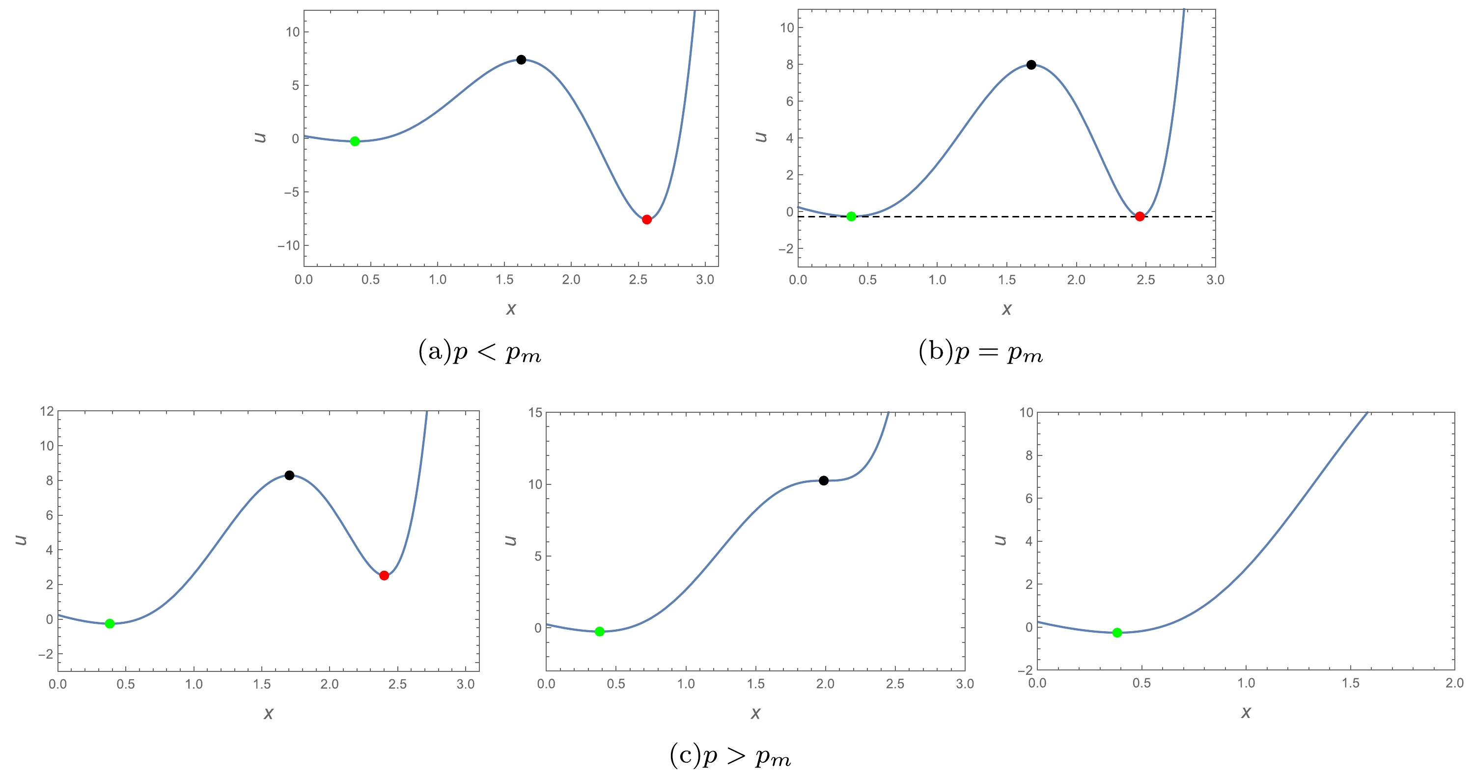
Figure 4. (color online)
$ u-x $ plots of$t=0.8 $ for$d = 7 $ . The$\color{green}{\bullet} $ -phase in the diagram represents the small black hole state,$\color{red}{\bullet} $ -phase represents the large black hole state, and$\bullet $ -phase represents the unstable black hole state. Pressure p increases from left to right in the$ p>p_m $ plots.When
$ p<p_m $ , the whole black hole system is completely in the large black hole phase, and conversely, the system is completely in the small black hole phase at$ p>p_m $ . There is also a critical point, Eq. (29), under this dimension. Therefore, it is concluded that the system will have first-order and second-order phase transitions. This is the same result as that calculated by the winding number. -
Let us now study the cases of 8, 9, 10, and 11 dimensions. From Eq. (26), it follows that the 8-, 9-, 10-, and 11-dimensional cases are similar. Therefore, we take the case of
$d=9 $ as an example. The analytic function is obtained by substituting$d=9 $ into Eq. (26), which reads as$ \begin{aligned}[b] f(z)=\;&\dfrac{1}{42\pi z(z^2+\alpha)^2}\bigg[24P\pi z^6+63z^4\\&+42\alpha z^2+7\alpha^2-42\pi zT( z^2+\alpha)^2\bigg]. \end{aligned} $

(31) There are four zeroes at most on complex plane
$ {\bf{C}}\backslash\{\pm \sqrt{\alpha}{\rm i}, 0\} $ . Hence, the winding number is W=4 and the complex structure is the Riemann surface with four foliations.According to the basic elements of the corresponding relationship between the winding number and phase transition, we can find that
$ W =4 $ can be decomposed in two ways: (i)$ 4=2+2 $ , which means that the system only has two second-order phase transitions; and (ii)$ 4 =1+3 $ , which shows that the system has one first-order and one second-order phase transitions. A clearer breakdown is shown in Fig. 5. Thus, we conjecture that in$d=9 $ , there will be two different types of phase transitions.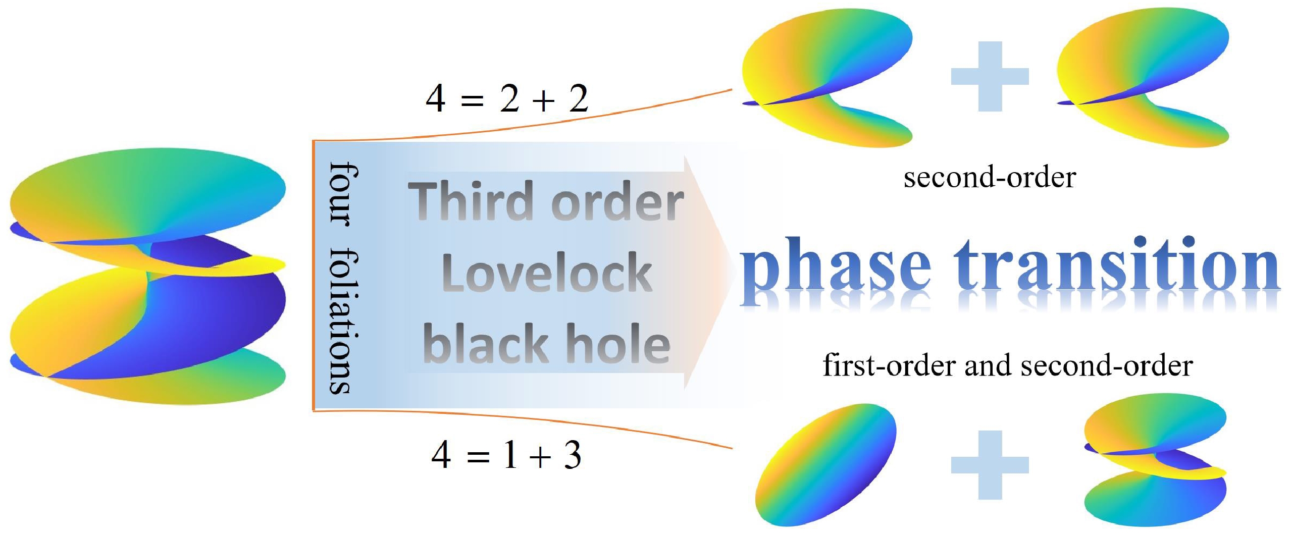
Figure 5. (color online) Two decompositions with winding number W = 4.
For the case of
$ d > 7 $ , there are two pairs of critical points for the system. This makes dimensionless processing more complicated, so we do not do this here, which is slightly different from the previous analysis. The two sets of critical points in$ d= 9 $ were obtained from [48], and they can be written as$ \begin{aligned}[b] P_{c1}=\;&\frac{7[(17 \sqrt{21}-105) \alpha^2+6(17 \sqrt{21}-77) \alpha+147-27 \sqrt{21}]}{8 \pi(367 \sqrt{21}-1687)}, \\ T_{c1}=\;&\frac{3\sqrt{3}( \sqrt{21}-7)}{\sqrt{\alpha}\pi \sqrt{6-\sqrt{21}} (\sqrt{21} -21)}, \\ v_{c1}=\;&\frac{4 \sqrt{\alpha} \sqrt{18-3 \sqrt{21}}}{21}, \end{aligned} $

(32) and
$ \begin{aligned}[b] P_{c2}=&\frac{7[(17 \sqrt{21}+105) \alpha^2+6(17 \sqrt{21}+77) \alpha-147-27 \sqrt{21})]}{8 \pi(367 \sqrt{21}+1687)} ,\\ T_{c2}=\;&\frac{3\sqrt{3}( \sqrt{21}+7)}{\sqrt{\alpha}\pi \sqrt{6+\sqrt{21}} (\sqrt{21} +21)}, \\ v_{c2}=\;&\frac{4 \sqrt{\alpha} \sqrt{18+3 \sqrt{21}}}{21}. \end{aligned} $

(33) The thermal potential is expressed with the help of Eq. (18) as
$ \begin{aligned}[b] U=\;&\frac{1}{4}\Bigg[\frac{7}{12\pi}\left(\frac{6}{7}\pi P r_h^8+3r_h^6+3\alpha r_h^4+\alpha^2r_h^2\right)\\&-T\left(r_h^7+\frac{14}{5}\alpha r_h^5+\frac{7}{3}\alpha^2r_h^3\right)\Bigg].\end{aligned} $

(34) For the sake of simplicity, we set both
$ \alpha=1 $ . By analysis, we find that the phase transition between the two critical temperatures needs to be discussed on a case-by-case basis.a.
$ T_{c1}\le T< T_{cm} $ As can be observed from Fig. 6, there is a gradual merging between the extremal points until they disappear as pressure P increases. During this time, the large black hole phase is always a global minimum and there is no transition between the two minima. This means that the system has no first-order phase transition. Instead, the system has a second-order phase transition due to the presence of the inflection point Eq. (32).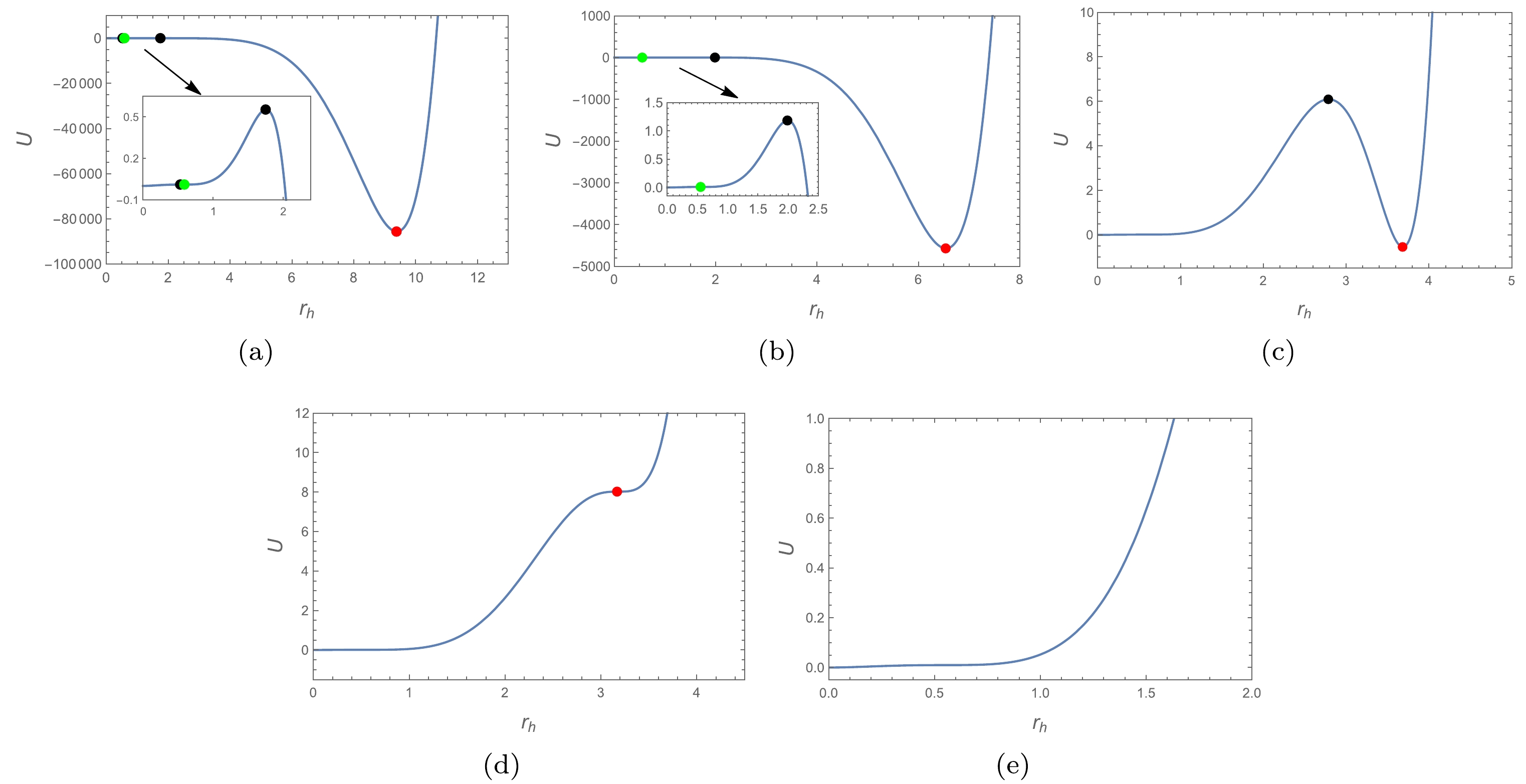
Figure 6. (color online)
$ U-r_h $ plots of$ T =0.2075 $ for$d=9 $ . The$\color{green}{\bullet} $ -phase in the diagram represents the small black hole state,$\color{red}{\bullet} $ -phase represents the large black hole state, and$ {\bullet} $ -phase represents the unstable black hole state. Pressure P increases from diagrams (a) to (e).b.
$ T=T_{cm} $ From Fig. 7, it can be observed that the thermal potential changes similarly to that of$ T<T_{cm} $ at both$ P<P_m $ and$ P>P_m $ . It is worth noting that at$ P=P_m $ , the global minimum and local minimum become two equal global minima, a phenomenon that does not exist for$ T<T_{cm} $ . Therefore,$ T_{cm} $ is the point at which the phase transition will begin to occur, which is still a second-order phase transition.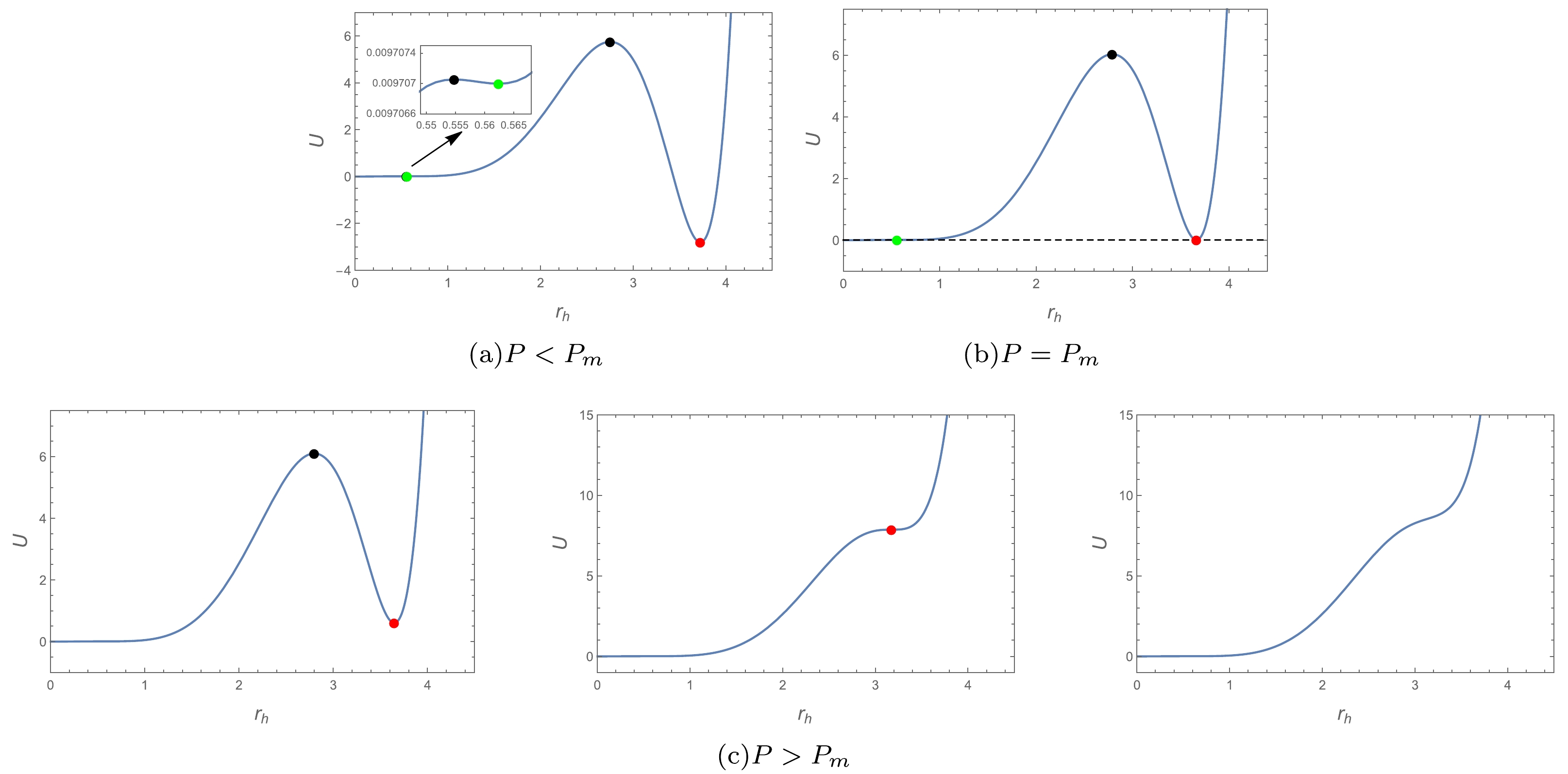
Figure 7. (color online)
$ U-r_h $ plots of$ T=T_{cm} $ for$d=9 $ . The$\color{green}{\bullet} $ -phase in the diagram represents the small black hole state,$\color{red}{\bullet} $ -phase represents the large black hole state, and$ {\bullet} $ -phase represents the unstable black hole state. Pressure P increases from left to right in the$ P>P_m $ plots.c.
$ T_{cm}<T\le T_{c2} $ As can be observed from diagrams (a) to (b) in Fig. 8, as pressure P starts to rise, the global minimum of the large black hole phase and the local minimum of the small black hole phase change to two equivalent global minima. The black hole system changes from a large black hole phase to co-existing large and small black hole phases. From diagrams (b) to (d), the pressure continues to increase from$ P_m $ and the two global minima are transformed into a global minimum and local minimum until the local minima disappear. The thermal potential of the small black hole phase is lower than that of the large black hole phase, which means that the system tends toward the small black hole phase. From the above analysis, it is clear that the system has a first-order phase transition. Meanwhile, due to the inflection point Eq. (33), it also has a second-order phase transition.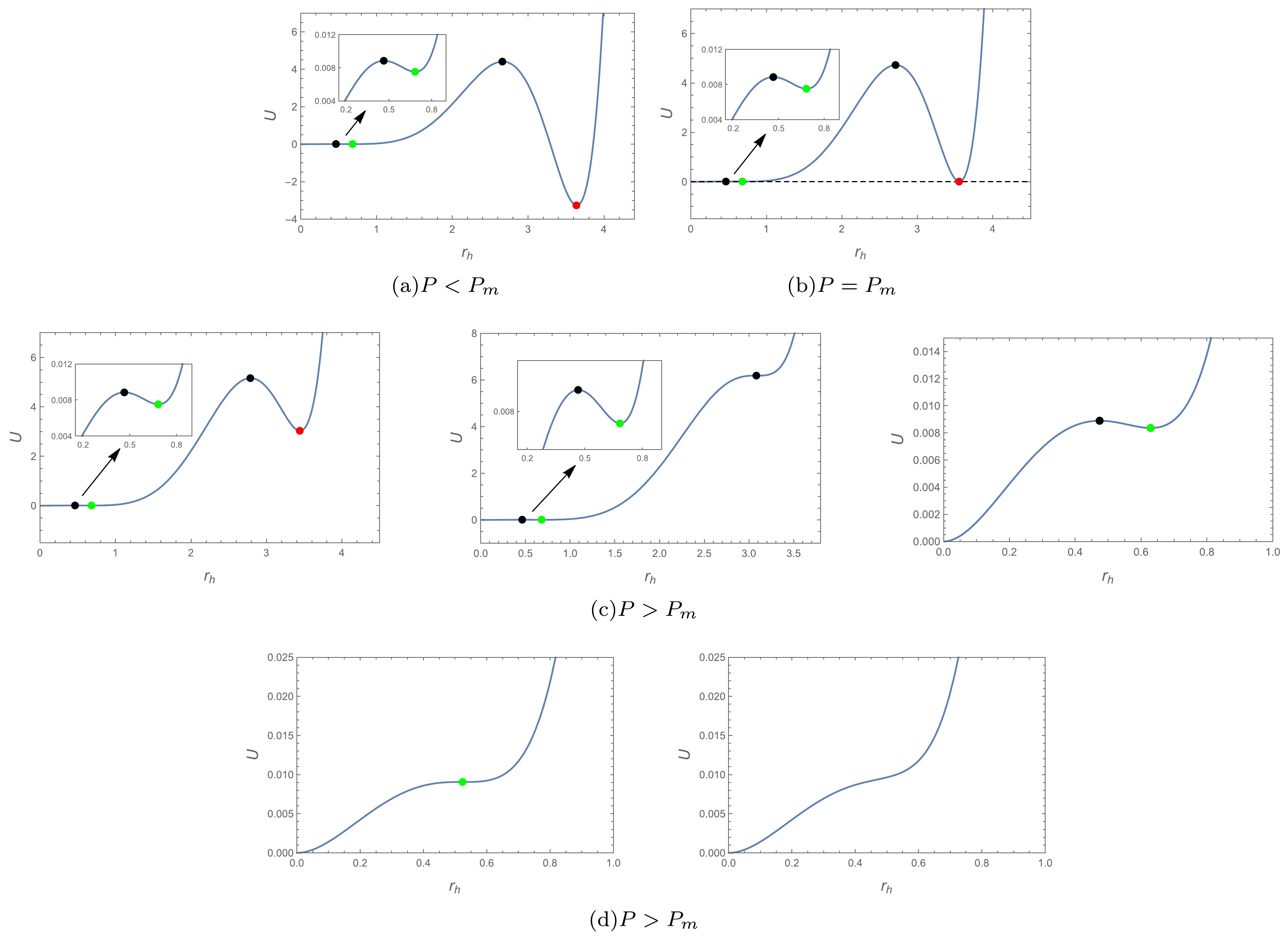
Figure 8. (color online)
$ U-r_h $ plots of$T=0.21 $ for$d=9 $ . The$\color{green}{\bullet} $ -phase in the diagram represents the small black hole state,$\color{red}{\bullet} $ -phase represents the large black hole state, and$ {\bullet} $ -phase represents the unstable black hole state. Pressure p increases from left to right in the$ P>P_m $ plots.We conclude from the thermal potential diagrams that there are indeed two different phase transition processes in d = 9, perfectly verifying the previous conjecture.
-
In this paper, the complex structure of the third-order Lovelock black hole phase transition is predicted by the local winding number, and its accuracy is verified by the behavior of the thermal potential. By transposing the complex analysis from mathematics to study the microstructure of the black hole thermodynamics and relating the winding number to the type of phase transitions, it is easy to know the order of the different phase transitions of the black hole.
In the hyperbolic case of arbitrary dimensions and the spherical case of 7 dimensions, the winding number is
$W=3 $ and the complex structure is the Riemann surface with three foliations, which indicates that there are first-order and second-order phase transitions in this system. The winding number is$W=4 $ in$ 7<d < 12 $ for the spherical case and the corresponding complex structure is the four-foliations Riemann surface.The thermal potential is next used to explore specifically how a black hole changes from one state to another. The thermal potential of the systems with varying pressure reveals different properties. Based on the nature of the thermal potential, the phase transition processes of Lovelock black holes under different topologies are analyzed.
For
$ k=-1 $ , the system has first-order and second-order phase transitions.For
$ k=+1 $ , the situation is slightly more complicated. The phase transition process in 7 dimensions is similar to that of the hyperbolic case, in which the first-order and second-order phase transitions also occur. Meanwhile, in 8, 9, 10, 11 dimensions, there is the key intermediate temperature,$ T_{cm} $ . When the temperature is$ T_{c1}<T< T_{cm} $ , there are only second-order phase transitions, and when$ T_{cm}<T< T_{c2} $ , the system has both second-order and first-order phase transitions. The winding number indicates the following:(i) 4=2+2 states that only second-order phase transition occurs. It is of this type when the temperature is between
$ T_{c1} $ and$ T_{cm} $ for the Lovelock black holes in the spherical topology of$ d>7 $ dimensions.(ii) 4=1+3 indicates that the system has both first-order and second-order phase transitions. It occurs when the temperature is between
$ T_{cm} $ and$ T_{c2} $ for the Lovelock black holes in the spherical topology of$ d>7 $ dimensions.The results of the above thermal potential analysis perfectly match the winding number prediction. By establishing the connection between the winding number and black hole phase transition, we obtain the complex phase transition structure. Complex analysis is an effective method to further study the microstructure of black hole systems. We hope that this work will provide new ideas for the study of black hole thermodynamic phase transitions, and thus further enrich the content of black hole thermodynamics.
In addition, when the winding number is
$W=3 $ , and there exists a first-order and second-order phase transition according to the present work, why do we not consider the case of$W=3 $ as a third-order phase transition directly? As far as our present work is concerned, on the one hand, our correspondence between winding number W and the phase transition of black holes is only a speculative and empirical construct based on some typical black hole thermodynamic systems, and the thermodynamic phase transitions of these black holes are either first-order or second-order. On the other hand, based on the current understanding, we have not encountered an example of the third-order phase transition in black hole thermodynamic systems. If there are, we will explore the situation where the system undergoes a third-order phase transition and its corresponding winding number. This requires further in-depth understanding and research in the future. -
The authors would like to thank the anonymous referee for the helpful comments that improve this work greatly.
Thermodynamic phase transition and winding number for the third-order Lovelock black hole
- Received Date: 2024-03-13
- Available Online: 2024-09-15
Abstract: Phase transition is important for understanding the nature and evolution of the black hole thermodynamic system. In this study, we predicted the phase transition of the third-order Lovelock black hole using the winding numbers in complex analysis, and qualitatively validated this prediction by the generalized free energy. For the 7<d<12-dimensional black holes in hyperbolic topology and the 7-dimensional black hole in spherical topology, the winding number obtained is three, which indicates that the system undergoes first-order and second-order phase transitions. For the 7<d<12-dimensional black holes in spherical topology, the winding number is four, and two scenarios of phase transitions exist, one involving a purely second-order phase transition and the other involving simultaneous first-order and second-order phase transitions. This result further deepens the research on black hole phase transitions using the complex analysis.


 DownLoad: