


 Abstract
 HTML
HTML Reference
 Related
 PDF
PDF


-
Since the Higgs was discovered by the ATLAS and CMS collaborations in 2012 [1, 2], many questions regarding its properties remain unanswered. According to the latest experimental data, the measured mass of the Higgs boson is [3]
$ \begin{array}{*{20}{l}} m_h = 125.25 \pm 0.17 \; {{\rm{GeV}}}. \end{array} $

As a new elementary particle, h is largely consistent with the neutral Higgs boson predicted by the standard model (SM). However many questions have been raised that challenge the SM framework.
Weak scale supersymmetry (SUSY) is a promising extension of the SM. It naturally explains why the electroweak (EW) symmetry breaking scale is much smaller than the Planck scale and solves the gauge hierarchy problem [4, 5]. However, the minimum supersymmetric SM (MSSM) cannot fully solve the hierarchy problem. Moreover, it has another problem named ''the μ problem''. Hence, extensions of the MSSM have been proposed to solve these problems. For example, an extension of the MSSM by adding a (SM) gauge singlet that is coupled to Higgs doublets (the NMSSM) has been proposed to solve the μ problem.
Unfortunately, the NMSSM with all the couplings being perturbative up to the GUT scale also does not really solve the little hierarchy problem [6−9]. If the little hierarchy problem is taken seriously, then one should consider another source of Higgs quadruple coupling, which will not decouple in the large
$ \tan\beta $ limit [10]. The model that extends the MSSM by adding$ S U$ (2) triplets, the triplet extended NMSSM (TMSSM) [11−13], possesses such a Higgs quartic coupling naturally.The combined advantages of NMSSM and TNMSSM can solve each other's problems [10]. In the TNMSSM, the singlet interactions do not play any important role in raising the physical Higgs mass: one relies on triplets instead of achieving this goal, and hence, one does not face the usual little hierarchy problems of the NMSSM.
This work study the 125 GeV SM-like Higgs boson decay
$ h\rightarrow MZ $ in the framework of TNMSSM, with M representing the mesons ρ, ω, ϕ,$ J/\psi $ , and Υ. The$h\rightarrow MZ$ decay has been shown in [14−20] via the effective vertex$ hZ\gamma^* $ and subsequent transition to$ \gamma^*\rightarrow M $ . No$ hZ\gamma $ coupling exists at tree level, but it can be contributed by the loop diagram [14]. The first evidence for the$ h\rightarrow \gamma Z $ process was presented by the ATLAS and CMS collaborations. The obseved signal strength at the$ 68\% $ confidence level is$ \mu=2.2^{+1.0}_{-0.9} $ for the ATLAS analysis,$\mu= 2.4^{+1.0}_{-0.9}$ for the CMS analysis, and$ \mu=2.2\pm0.7 $ for their combination [21]. The$ h\rightarrow \gamma Z $ process has been observed, and the results are shifted from the SM. This presupposes the existence of a new physics, whose contribution to the process may be able to explain the deviations between the observed decays and SM predictions, and thus the associated decay process deserves to be investigated. This coupling is important for probing a new physics. In the TNMSSM, additional coupling exists of the Higgs boson to additional charged scalars and charged fermions. They contribute to the$ hZ\gamma $ coupling through loop diagrams.This paper is organized as follows. We briefly present the main ingredients of the TNMSSM in Sec. II. We present the Higgs boson decay
$ h\rightarrow Z\gamma $ and$ h\rightarrow MZ $ formulas in Sec. III. We show the input parameters and numerical results in Sec. IV. In the last section, we present the discussion and conclusion. Finally, some related formulas are included in the Appendix. -
Compared to the MSSM, the TNMSSM includes two new
$S U $ (2)$ _L $ triplet superfields T,$ \bar T $ with hypercharge ±1 and an SM gauge singlet superfield$ \hat s $ , which are coupled to each other.The superpotential of the TNMSSM can be written as follows:
$ \begin{aligned}[b] W=\;&-Y_d\hat d\hat q\hat H_d-Y_e\hat e\hat l\hat H_d+\chi_d\hat H_d \hat T\hat H_d+\lambda\hat H_u\hat H_d \hat s+\chi_t\hat H_u\hat{\bar{T}}\hat H_u\\&+\frac13\kappa\hat s^3+\Lambda_T\hat s\hat{\bar T}\hat T+Y_u\hat u\hat q\hat H_u \,. \end{aligned} $

Here, the triplet superfields with hypercharge Y = ±1 are defined as
$ \begin{array}{*{20}{l}} T\equiv T^a\sigma ^a= \begin{pmatrix} T^+/\sqrt{2}&-T^{++}\\ T^0&-T^+/\sqrt{2} \end{pmatrix}\\ \bar{T}\equiv \bar{T}^a\sigma^a= \begin{pmatrix} \bar{T}^-/\sqrt{2}&-\bar{T}^{0}\\ \bar{T}^{-}&-\bar{T}^-/\sqrt{2} \end{pmatrix} \end{array} $

The soft SUSY breaking terms are as follows:
$ \begin{aligned}[b] -\mathcal{L}_{\rm soft}=\;& \frac{1}{2}(M_1\lambda_1\lambda_1+M_2\lambda_2\lambda_2+M_3\lambda_3\lambda_3 +h.c.)+m_{Hu}^2|H_u|^2+m_{H_d}^2|H_d|^2+m_{\bar T}^2Tr(\bar T^\dagger\bar T) + m_T^2Tr(T^\dagger T)+m_S^2|S|^2 +m_{\tilde{Q}}^2|\tilde{Q}|^2\\ &+m_{\tilde{u}}^2|\tilde{u}_R|^2+m_{\tilde{d}}^2|\tilde{d}_R|^2+m_{\tilde{l}}^2|\tilde{l}|^2+m_{\tilde{e}}^2|\tilde{e}_R|^2+ (T_{\Lambda T} tr(T\bar T)S+T_{\chi d}H_d\cdot TH_d+T_{\chi_t}H_u\cdot\bar{T}H_u+\frac{T_{\kappa}}{3}S^3+T_{\lambda}H_u\cdot H_dS\\&+ T_dH_d\cdot \tilde{Q}d^*-T_uH_u\cdot \tilde{Q}u^*+T_eH_d\cdot Le^*+ {\rm h.c.}), \end{aligned} $ 
(1) where the respective definitions of the products between the two
$S U(2)_L$ doublets and between the$ S U(2)_L $ doublets and$ S U(2)_L $ triplet are given as follows:$ \begin{aligned}[b]& H_u\cdot H_d=H_u^+H_d^-H_u^0H_d^0,\\ & H_u\cdot \bar{T}H_u=\sqrt{2}H_u^0H_u^+\bar{T}^-(H_u^0)^2\bar{T}^0-(H_u^+)^2\bar{T}^{-},\\& H_d\cdot TH_d=\sqrt{2}H_d^0H_d^-T^+-(H_d^0)^2T^0-(H_d^-)^2T^{++}. \end{aligned} $

Once the electroweak symmetry is spontaneously broken, the neutral scalar fields can be defined as
$ \begin{aligned}[b]& \langle H_u^0\rangle=\frac{v_u+\phi_u+{\rm i}\sigma_u}{\sqrt{2}}, \qquad \langle H_d^0\rangle=\frac{v_d+\phi_d+{\rm i}\sigma_d}{\sqrt{2}},\\ & \langle T^0\rangle=\frac{v_T+\phi_T+{\rm i}\sigma_T}{\sqrt{2}},\qquad \langle\bar{T}^0\rangle=\frac{\bar{v}_T+\phi_{\bar{T}}+{\rm i}\sigma_{\bar{T}}}{\sqrt{2}},\\ & \langle S\rangle=\frac{v_s+\phi_s+{\rm i}\sigma_s}{\sqrt{2}}. \end{aligned} $

We define the ratio
$ v_u $ to$ v_d $ as$ \tan\beta=\dfrac{v_u}{v_d} $ , and the ratio$ v_T $ to$ v_{\bar T} $ as$ \tan\beta'=\dfrac{v_T}{v_{\bar T}} $ .Because we introduce a single state and two triplet states, we have five minimization equations, including the usual upper and lower Higgs. In general, the vacuum expectation value of the triplet states must be small to avoid large ρ-parameter corrections [10].
In the basis
$ (H_d^-,H_u^{+,*},\bar T^-,T^{+,*}) $ and$ (H_d^{-,*},H_u^+,\bar T^{-,*},T^+) $ , the definition of the mass squared matrix for a charged Higgs is given by$ \begin{array}{*{20}{l}} m_{H^-}^2=\begin{pmatrix} m_{H_d^-,H_d^{-,*}}&m_{H_u^{+,*},H_d^{-,*}}^*&m_{\bar T^-,H_d^{-,*}}^*&m_{T^{+,*},H_d^{-,*}}^*\\ m_{H_d^-,H_u^+}&m_{H_u^{+,*},H_u^+}&m_{\bar T^-,H_u^+}^*&m_{T^{+,*},H_u^+}^*\\ m_{H_d^-,\bar T^{-,*}}&m_{H_u^{+,*}\bar T^{-,*}}&m_{\bar T^-\bar T^{-,*}}&m_{T^{+,*}\bar T^{-,*}}^*\\ m_{H_d^-,T^+}&m_{H_u^{+,*}T^+}&m_{\bar T^-T^+}&m_{T^{+,*}T^+} \end{pmatrix} \end{array} $

(2) where
$\begin{aligned}\\[-12pt] m_{H_d^-,H_d^{-,*}}= \frac{1}{2}v_s^2|\lambda|^2+\frac{1}{8}\big[g_1^2(2v_{\bar T}^2-2v_T^2-v_u^2+v_d^2)+g_2^2(-2v_{\bar T}^2+2v_T^2+v_d^2+v_u^2)\big]+v_d^2|\chi_d|^2+m_{H_d}^2,\end{aligned} $ 
$ \begin{aligned}[b] m_{H_d^-,H_u^+}=\;& \frac{1}{2}\big[\lambda(-v_dv_u\lambda^*+v_s^2\kappa^*-v_Tv_{\bar T}\Lambda_T^*)+\sqrt{2}v_sT_{\lambda}\big]+\frac{1}{4}g_2^2v_dv_u,\\ m_{H_u^{+,*},H_u^+}=\;& \frac{1}{2}v_s^2|\lambda|^2+\frac{1}{8}\big[(g_1^2+g_2^2)v_u^2-(-g_2^2+g_1^2)(2v_{\bar T}^2-2v_T^2+v_d^2)\big]+v_u^2|\chi_t|^2+m_{H_u}^2,\\ m_{H_d^-,\bar T^{-,*}}=\;& \frac{1}{2\sqrt{2}}g_2^2v_dv_{\bar T}-\frac{1}{\sqrt{2}}v_s(v_d\chi_d\Lambda_T^*+v_u\lambda\chi_t^*),\\ m_{H_u^{+,*}\bar T^{-,*}}=\;& \frac{1}{2\sqrt{2}}g_2^2v_{\bar T}v_u+\frac{1}{\sqrt{2}}(-2v_{\bar T}v_u\chi_t+v_dv_s\lambda)\chi_t^*-v_uT_{\chi,t^*},\\ m_{\bar T^-\bar T^{-,*}}=\;& \frac{1}{2}v_s^2|\Lambda_T|^2+\frac{1}{4}\big[2g_2^2v_{\bar T}^2+(g_1^22v_{\bar T}^2-2v_T^2-v_u^2+v_d^2)\big]+v_u^2 |\chi_t|^2+m_{\bar T}^2,\\ m_{H_d^-,T^+}=\;& \frac{1}{2\sqrt{2}}g_2^2v_dv_T+\frac{1}{\sqrt{2}}v_sv_u\chi_d\lambda^*-v_d(\sqrt{2}v_T|\chi_d|^2+T_{\chi_d}),\\ m_{H_u^{+,*}T^+}=\;& \frac{1}{2\sqrt{2}}g_2^2v_dv_u-\frac{1}{\sqrt{2}}v_s(\Lambda_T v_u\chi_t^*+v_d\chi_d\lambda^*),\\ m_{\bar T^-T^+}=\;& \frac{1}{2}g_2^2v_Tv_{\bar T}+\frac{1}{2}\big[\Lambda_T(-v_dv_u\lambda^*+v_s^2\kappa^*-v_Tv_{\bar T}\Lambda_T^*)+\sqrt{2}v_sT_{\Lambda_T}\big],\\ m_{T^{+,*}T^+}=\;& \frac{1}{2}v_s|\Lambda_T|^2+\frac{1}{4}\big[2g_2^2v_T^2+g_1(-2v_{\bar T}^2+2v_T^2-v_d^2+v_u^2)\big]+v_d^2|\chi_d|^2+m_T^2. \end{aligned} $

This matrix is diagonalized by
$ Z^+ $ :$ \begin{array}{*{20}{l}} Z^+m_{H^-}^2Z^{+,\dagger}=m_{2,H^-}^{\rm dia} \end{array} $

with
$ \begin{aligned}[b]& H_d^-=\sum\limits_jZ_{j1}^+H_j^-,\; \; \; H_u^+=\sum\limits_jZ_{j2}^+H_j^+,\\& T^-=\sum\limits_jZ_{j3}^+H_j^-,\; \; \; T^+=\sum\limits_jZ_{j4}^+H_j^+. \end{aligned} $

The mass of the SM-like Higgs boson in the TNMSSM can be written as
$ \begin{array}{*{20}{l}} m_h=\sqrt{(m^0_{h_1})^2+\Delta m_h^2} \; , \end{array} $

(3) where
$ m^0_{h_1} $ is the lightest tree-level Higgs boson mass, and$ \Delta m^2_h $ is the radiative correction. The two-loop leading-log radiative corrections can be given as$ \begin{aligned}[b] \Delta m^2_h=\;&\frac{3m_t^4}{4\pi^2v^2}\left[\left(\tilde{t}+\frac{1}{2}\tilde{X}_t\right)+\frac{1}{16\pi^2}\left(\frac{3m_t^2}{2v^2}-32\pi\alpha_3\right)\right.\\&\times\left(\tilde{t}^2+\tilde{X}_t\tilde{t}\right)\Bigg],\end{aligned} $

(4) $ \tilde{t}=\log\frac{M^2_S}{m^2_t},\qquad \tilde{X}_t=\frac{2\tilde{A}_t^2}{M_S^2}\left(1-\frac{\tilde{A}_t^2}{12M_S^2}\right), $

(5) where
$ \alpha_3 $ is the running strong coupling constant.$ M_S= \sqrt{m_{\tilde{t}_1}m_{\tilde{t}_2}} $ , where$ m_{\tilde{t}_{1,2}} $ are the stop masses.$ \tilde{A}_t=A_t - \mu\cot\beta $ , with$ A_t=T_{u,33}/Y_{u,33} $ . -
In this section, we discuss the Higgs boson decay processes
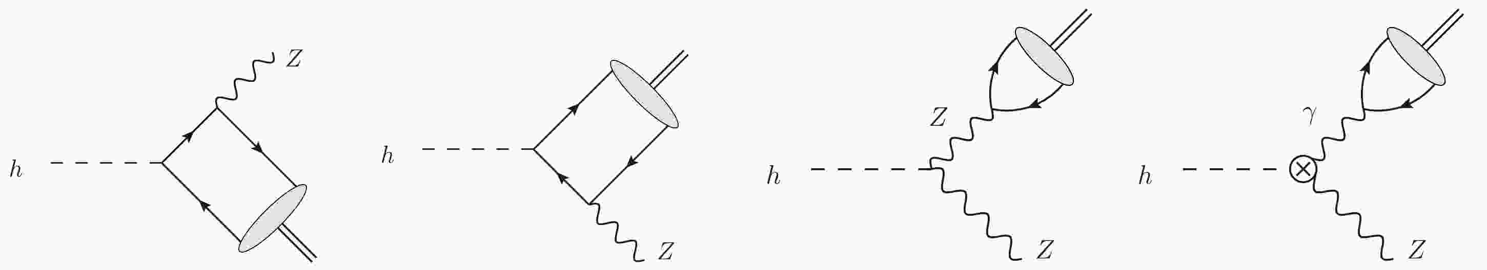
$ h\rightarrow Z\gamma $ and$ h\rightarrow MZ $ . The dominating Feynman diagrams for$ h\rightarrow MZ $ are shown in Fig. 1. The first two diagrams in Fig. 1 are the direct contributions, and the last two diagrams represent the indirect contributions. For the indirect contribution, there is a process$ h\rightarrow Z\gamma^*\rightarrow MZ $ , where$ \gamma^* $ is off-shell and changes into the final state meson.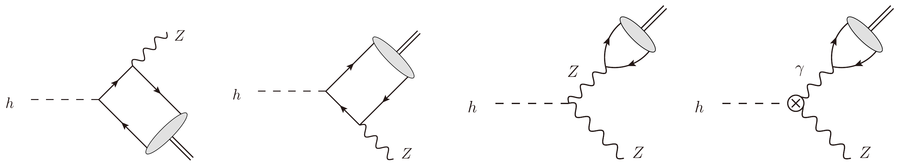
Figure 1. Diagrams contributing to the decay
$ h\rightarrow MZ $ . The crossed circle in the last graph represents the effective vertex$ h\rightarrow Z\gamma^* $ from the one loop diagrams.There is no contribution to
$ hZ\gamma $ coupling at the tree level in the TNMMSM, but it can be created by loop diagrams. The$ h\rightarrow Z\gamma^* $ process can be used to probe for a new physics. Thus, we will focus on discussing$ h\rightarrow Z\gamma^* $ . In the TNMSSM, the non-standard$ h^0\gamma Z $ vertex should be taken into account. The effective Lagrangian for$ h\gamma Z $ is written as$ \mathcal{L}_{eff}=\frac{\alpha}{4\pi \upsilon}\Bigg(\frac{2C_{\gamma Z}}{s_Wc_W}hF_{\mu\nu}Z^{\mu\nu} -\frac{2\tilde{C}_{\gamma Z}}{s_Wc_W}hF_{\mu\nu}\tilde{Z}^{\mu\nu} \Bigg), $

(6) with
$ s_W=\sin\theta_W, c_W=\cos\theta_W $ . The decay width of$ h\rightarrow Z\gamma $ deduced by the effective Lagrangian defined in Eq. (6) is$ \Gamma(h\rightarrow Z\gamma)=\frac{\alpha^2m_{h^0}^3}{32\pi^3\upsilon^2s_W^2c_W^2}\left(1-\frac{m_Z^2}{m_{h^0}^2}\right)^3(|C_{\gamma Z}|^2+|\tilde{C}_{\gamma Z}|^2). $

(7) The loop diagrams make additional contributions to
$ h\rightarrow MZ $ decays in the new physics. The decay width of$ h\rightarrow MZ $ is given by$ \begin{aligned}[b] & \Gamma(h\rightarrow MZ)=\frac{m_{h^0}^3}{4\pi \upsilon^4}\,\lambda^{1/2}(1,r_Z,r_M)\,(1-r_Z-r_M)^2 \\ &\quad\times \left[ \big| F_\parallel^{MZ} \big|^2 + \frac{8r_M r_Z}{(1-r_Z-r_M)^2} \Big( \big| F_\perp^{MZ} \big|^2 + \big| \tilde F_\perp^{MZ} \big|^2 \Big) \right] , \end{aligned} $

(8) with
$ \lambda(x,y,z)=(x-y-z)^2-4yz,r_Z=\dfrac{m_Z^2}{m_h^2} $ .$ r_M=\dfrac{m_M^2}{m_h^2} $ , and$ m_M $ is the mass of a vector meson.$ F_{\parallel}^{MZ} $ and$ F_{\perp}^{MZ} $ represent the CP-even longitudinal and transverse form factors, respectively.$ \tilde F_{\perp}^{MZ} $ represents the CP-odd transverse form factors. For the vector mesons considered in this work, the mass ratio$ r_M $ is very small, but it can make significant contributions to the transverse polarization states. To obtain better results, we maintain it in our study.In Eq. (8),
$ F_{\parallel}^{MZ}, F_{\perp}^{MZ} $ , and$ \tilde F_{\perp}^{MZ} $ could be divided into direct and indirect parts. The indirect contributions are as follows:$ \begin{aligned}[b]F_{\parallel\, \rm indirect}^{MZ}=\;& \frac{\kappa_Z}{1-r_M/r_Z} \sum\limits_q f_M^q\,v_q + C_{\gamma Z}\,\frac{\alpha_s (m_M)}{4\pi}\,\\&\times\frac{4r_Z}{1-r_Z-r_M} \sum\limits_q f_M^q\,Q_q , \end{aligned} $

(9) $ \begin{aligned}[b]F_{\perp\, \rm indirect}^{MZ}=\;&\frac{\kappa_Z}{1-r_M/r_Z} \sum\limits_q f_M^q\,v_q + C_{\gamma Z}\,\frac{\alpha_s (m_M)}{4\pi}\,\\&\times\frac{1-r_Z-r_M}{r_M} \sum\limits_q f_M^q\,Q_q , \end{aligned} $

(10) $ \tilde F_{\perp\, \rm indirect}^{MZ}=\tilde C_{\gamma Z}\,\frac{\alpha_s (m_M)}{4\pi}\,\frac{\lambda^{1/2}(1,r_Z,r_M) }{r_M} \sum\limits_q f_M^q\,Q_q , $

(11) where
$ v_q=\dfrac{T_3^q}{2}-Q_q\sin^2 \theta_W $ represents the vector couplings of the Z boson to the quark q.$ \kappa_Z $ is the ratio of the coupling of the SM-like Higgs boson to Z boson to the corresponding SM value.$ \alpha_s $ is the strong coupling constant. The flavor-specific decay constants$ f_M^q $ are defined by$ \begin{array}{*{20}{l}} \langle M(k,\varepsilon)|\bar q\gamma^\mu q|0\rangle=-{\rm i}f_M^qm_M\varepsilon^{*\mu},\; \; \; \; \; q=u,d,s\dots \end{array} $

(12) The calculations can be simplified by the following relationship:
$ \begin{array}{*{20}{l}} \sum\limits_q f_M^qQ_q=f_MQ_M, \; \; \; \; \; \; \sum\limits_q f_M^qv_q=f_Mv_M. \end{array} $

(13) The vector meson decay constants
$ f_M, Q_M, v_M $ are listed in Table 1.Vector meson ω ρ ϕ $ J/\psi $ 

Υ $ m_M/{{\rm{GeV}}} $ 

0.782 0.77 1.02 3.097 9.46 $ f_M/{{\rm{GeV}}} $ 

0.194 0.216 0.223 0.403 0.684 $ v_M $ 

$ -\dfrac{\sin^2\theta_W}{3 \sqrt{2}} $ 

$ \dfrac{1}{\sqrt{2}} (\dfrac{1}{2}-\sin^2\theta_W) $ 

$ -\dfrac{1}{4}+\dfrac{\sin^2\theta_W}{3} $ 

$ \frac{1}{4}-\dfrac{2 \sin^2\theta_W}{3} $ 

$ -\dfrac{1}{4}+\dfrac{\sin^2\theta_W}{3} $ 

$ Q_M $ 

$ \dfrac{1}{3 \sqrt{2}} $ 

$ \dfrac{1}{\sqrt{2}} $ 

$ -\dfrac{1}{3} $ 

$ \dfrac{2}{3} $ 

$ -\dfrac{1}{3} $ 

$ {f^{\perp}_M}/{f_M}={f^{q \perp}_M}/{f^{q}_M} $ 

0.71 0.72 0.76 0.91 1.09 Table 1. Mesons decay constants
$ f_M $ ,$ Q_M $ ,$ v_M $ used in the numerical analysis, where$ f_M^{\perp} $ and$ f_M^{q\perp} $ represent the transverse decay constants and flavor-specific transverse decay constants, respectively.The concrete forms of
$ C_{\gamma Z} $ and$ \tilde C_{\gamma Z} $ in Eqs. (9)–(11) can be written as [16, 17, 22]$ \begin{aligned}[b] C_{\gamma Z}=\;& C_{\gamma Z}^{\rm{SM}}+C_{\gamma Z}^{\rm{NP}}, \; \; \; \; \; \; \; \; \; \; \; \; \; \; \tilde C_{\gamma Z} = \tilde C_{\gamma Z}^{\rm{SM}}+\tilde C_{\gamma Z}^{\rm{NP}}.\\ C_{\gamma Z}^{\rm{SM}}=\;& \sum\limits_q \frac{2 N_c Q_q v_q}{3}\,A_f(\tau_q,r_Z) \\& + \sum\limits_l \frac{2 Q_l v_l}{3}\,A_f(\tau_l,r_Z) - \frac{1}{2}\,A_W^{\gamma Z}(\tau_W,r_Z),\\ \tilde{C}_{\gamma Z}^{\rm{SM}}=\;&\sum\limits_{q} \tilde{\kappa}_q N_c Q_q v_q B_f({\tau}_q,r_Z)+\sum\limits_{l} \tilde{\kappa}_l Q_l v_l B_f({\tau}_l,r_Z), \end{aligned} $

(14) where
$ \tau_i=\dfrac{4m_i^2}{m_h^2} $ ,$ v_l $ are the vector couplings of the Z boson to the leptons, and$ Q_l $ represents the charge of leptons.$ C_{\gamma Z}^{\rm SM} $ and$ \tilde{C}_{\gamma Z}^{\rm SM} $ represent the SM contributions to$ h\rightarrow Z\gamma $ .$ \tilde\kappa_q $ and$ \tilde{\kappa}_l $ represent the effective Higgs couplings to the quarks and leptons, respectively.$ A_f,\; B_f $ , and$ A_W^{\gamma Z} $ are loop functions that can be found in Refs. [18, 23]. The numerical values of$ C_{\gamma Z}^{\rm SM} $ and$ \tilde C_{\gamma Z}^{\rm SM} $ are taken as$C_{\gamma Z}^{\rm SM}\sim-2.395+0.001{\rm i},\; \tilde C_{\gamma Z}^{\rm SM}\sim0$ in Ref. [16].In the TNMSSM, the one loop diagrams contributing to
$ h\rightarrow \gamma Z $ are shown in Fig. 2, where F represents the charged Fermions and S represents the charged scalars. The new contributions to$ C_{\gamma Z} $ originate from the exchanged particles: charginos, sleptons, squarks, and charged Higgs.
Figure 2. One loop diagrams for
$ h\rightarrow \gamma Z $ in the TNMSSM, with$ F=\chi^{\pm},\chi^{\pm\pm} $ denoting the charged fermions and$ S=\tilde{u}_{i}^{+},\tilde{d}_{i}^{-},S_{\alpha}^{\pm},S_{\alpha}^{\pm\pm} $ denoting the squarks and charged scalars.The CP-odd coupling
$ \widetilde{C}_{\gamma Z} $ is 0 in the SM. In the TNMSSM, the$ h\gamma Z $ coupling can be written as$ \bar{F}_1 i(A+B\gamma^5)F_2h $ , where A is the CP-even part and B is the CP-odd part [16, 17]. For the interaction$ \bar{F}_1i(C^RP_R+ C^LP_L)F_2h $ with$ P_L=\dfrac{1-\gamma_5}{2} $ and$ P_R=\dfrac{1+\gamma_5}{2} $ , the CP-even part is$ A=\dfrac{1}{2}(C^L+C^R) $ and the CP-odd part is$B= \dfrac{1}{2}(C^R-C^L)$ . In the TNMSSM,$ \begin{array}{*{20}{l}} C^L_{hS^+S^-}=C^R_{hS^+S^-}, \; \; C^L_{hS^{++}S^{-}}=C^R_{hS^{++}S^{-}},\; \; C^L_{h\tilde{f}\tilde{f}}=C^R_{h\tilde{f}\tilde{f}},\\ C^L_{h\chi^+\chi^-}=C^R_{h\chi^+\chi^-},\; \; C^L_{h\chi^{++}\chi^{-}}=C^R_{h\chi^{++}\chi^{-}} \end{array} $

and only
$ C^L_{Z\chi^+\chi^-}\neq C^R_{Z\chi^+\chi^-} $ or$ C^L_{Z\chi^{++}\chi^{-}}\neq C^R_{Z\chi^{++}\chi^{-}} $ . However,$ C^L_{Z\chi^+\chi^-}+ C^R_{Z\chi^+\chi^-}\gg C^R_{Z\chi^+\chi^-}-C^L_{Z\chi^+\chi^-} $ ,$C^L_{Z\chi^{++}\chi^{-}}+C^R_{Z\chi^{++}\chi^{-}}\gg C^R_{Z\chi^{++}\chi^{-}}- C^L_{Z\chi^{++}\chi^{-}}$ . Thus, we can neglect the CP-odd coupling$ \widetilde{C}^{NP}_{\gamma Z} $ in the TNMSSM. The expression of CP-even coupling$ C^{NP}_{\gamma Z} $ in the TNMSSM is$ \begin{aligned}[b] C_{\gamma Z}^{NP}=\;&\dfrac{c_w}{2}\big[\sum\limits_{S^{\pm} }\left(2c_w^2-1\right)g_{hS^+S^-}(m_Z^2/m_{S^{\pm}}^2)A_0[x_{S^\pm},\lambda_{S^{\pm}}]\\ &+\sum\limits_{S^{\pm\pm}}\left(2c_w^2-1\right)g_{hS^{++}S^{-}}(m_Z^2/m_{S^{\pm\pm}}^2)A_0[x_{S^{\pm\pm}},\lambda_{S^{\pm\pm}}]\\ &+\sum\limits_{\tilde{f}}N_cQ_{\tilde{f}}\hat{v}_{\tilde{f}}g_{h\tilde{f}\tilde{f}}(m_Z^2/m_{\tilde{f}}^2)A_0[x_{\tilde{f}},\lambda_{\tilde{f}}]\\ &+\sum\limits_{\chi^{\pm};m,n=L,R}g^m_{h\chi^{\pm}\chi^{\mp}}g^n_{Z\chi^{\pm}\chi^{\mp}}(2m_W/m_{\chi^{\pm}})A_{1/2}[x_{\chi^\pm},\lambda_{\chi^\pm}]\\ &+\sum\limits_{\chi^{\pm\pm};m,n=L,R}g^m_{h\chi^{\pm\pm}\chi^{\mp\mp}}g^n_{Z\chi^{\pm\pm}\chi^{\mp\mp}}(2m_W/m_{\chi^{\pm\pm}})A_{1/2}[x_{\chi^\pm\pm},\lambda_{\chi^\pm\pm}]\big] \end{aligned} $

(15) where
$ x_i=4m_i^2/m_h^2 $ ,$ \lambda_i=4m_i^2/m_Z^2 $ ,$ \hat{v}_{\tilde{f}_1}=(T^f_3\cos^2\theta_f-Q_fs_w^2)/ c_w $ , and$ \hat{v}_{\tilde{f}_2}=(T^f_3\sin^2\theta_f-Q_fs_w^2)/c_w $ .$ \hat{v}_{\tilde{f}_1} $ and$ \hat{v}_{\tilde{f}_2} $ represent up and down-quark sectors.$ T_3^f $ is the weak isospin of fermion f,$ \theta_f $ is the mixing angle of sfermions$ \tilde{f}_{1,2} $ . The functions$ A_0 $ ,$ A_{1/2} $ can be found in [23, 24]. The concrete expressions of couplings are as follows:$ \begin{aligned}[b]& g_{hS^+S^-}=-\frac{v}{2m_Z^2}C_{hS^+S^-}^{L,R} ,\quad g_{hS^{++}S^{-}}=-\frac{v}{2m_Z^2}C_{hS^{++}S^{-}}^{L,R}\\& g_{h\tilde{f}\tilde{f}}=-\frac{v}{2m_Z^2}C_{h\tilde{f}\tilde{f}}^{L,R} ,\quad g_{h\chi^{\pm}\chi^{\mp}}^{L,R}=-\frac{1}{e}C_{h\chi^{\pm}\chi^{\mp}}^{L,R}\\& g_{Z\chi^{\pm}\chi^{\mp}}^{L,R}=-\frac{1}{e}C_{Z\chi^{\pm}\chi^{\mp}}^{L,R} ,\quad g_{h\chi^{\pm\pm}\chi^{\mp\mp}}^{L,R}=-\frac{1}{e}C_{h\chi^{\pm\pm}\chi^{\mp\mp}}^{L,R}\\& g_{Z\chi^{\pm\pm}\chi^{\mp\mp}}^{L,R}=-\frac{1}{e}C_{Z\chi^{\pm\pm}\chi^{\mp\mp}}^{L,R} . \end{aligned} $

As discussed in Ref. [25], the QCD corrections to the process
$ h\rightarrow Z\gamma $ are approximately$ 0.1\% $ , which indicates that the QCD corrections can be neglected safely. In other words, we can safely neglect the QCD corrections because they are very small.Compared to the indirect contributions, the direct contributions are very different, and they can be calculated in a power series
$ (m_q/m_h)^2 $ or$ (\Lambda_{\rm QCD}/m_h)^2 $ . For the transversely polarized vector meson, the leading-twist projections provide direct contributions. We can obtain the direct contributions by the asymptotic function$ \phi_M^{\perp}=6x(1-x) $ [26−28].$ F_{\perp\rm direct}^{MZ}=\sum\limits_qf_M^{q\perp}v_q\kappa_q\frac{3m_q}{2m_M}\frac{1-r_Z^2+2r_Z\ln r_Z}{(1-r_Z)^2}, $

(16) $ \tilde{F}_{\perp\rm direct}^{MZ}=\sum\limits_qf_M^{q\perp}v_q\tilde\kappa_q\frac{3m_q}{2m_M}\frac{1-r_Z^2+2r_Z\ln r_Z}{(1-r_Z)^2} . $

(17) In the calculations, it is found that the direct contribution is much smaller than the indirect contribution. This indicates that the indirect contributions are more important than the direct contributions. The contributions for the decay width of
$ h\rightarrow MZ $ in the SM are presented in Table 2.${\rho}$ 

ω ϕ J/ψ Υ $F_{\parallel {\rm{ind}}}^{MZ}$ 

${0.0423+4.3\times10^{-4}C_{\gamma Z}^{\rm{SM}}}$ 

${-0.0102+1.3\times10^{-4}C_{\gamma Z}^{\rm{SM}}}$ 

${-0.0392\\ -2.1\times10^{-4}C_{\gamma Z}^{\rm{SM}}}$ 

${0.041+7.5\times10^{-4}C_{\gamma Z}^{\rm{SM}}}$ 

${-0.115\\ -6.1\times10^{-4}C_{\gamma Z}^{\rm{SM}}}$ 

$F_{\perp {\rm{ind}}}^{MZ}$ 

${0.042+1.181C_{\gamma Z}^{\rm{SM}}}$ 

${-0.01+0.343C_{\gamma Z}^{\rm{SM}}}$ 

${-0.039\\ -0.327C_{\gamma Z}^{\rm{SM}}}$ 

${0.04+0.128C_{\gamma Z}^{\rm{SM}}}$ 

${-0.12\\ -0.011C_{\gamma Z}^{\rm{SM}}}$ 

$F_{\perp {\rm{direct}}}^{MZ}$ 

$0.0037$ 

$-0.00087$ 

$-0.00257$ 

$-0.00088$ 

$-0.00080$ 

Table 2. Contributions for the decay width of
$ h\rightarrow MZ $ in the SM, with$ C_{\gamma Z}^{\rm{SM}}\simeq-2.43 $ .Normalized to the SM expectation, the signal strengths for the Higgs decay channels can be quantified as
$ \mu^{ggF}_{MZ}=\frac{\sigma_{\rm NP}(ggF)Br_{\rm NP}(h\rightarrow MZ)}{\sigma_{\rm SM}(ggF)Br_{\rm SM}(h\rightarrow MZ)} , $

(18) $ \mu^{ggF}_{\gamma\gamma}=\frac{\sigma_{\rm NP}(ggF)Br_{\rm NP}(h\rightarrow \gamma\gamma)}{\sigma_{\rm SM}(ggF)Br_{\rm SM}(h\rightarrow \gamma\gamma)}, $

(19) where ggF stands for gluon-gluon fusion. The Higgs production cross sections can be written as
$ \frac{\sigma_{\rm NP}(ggF)}{\sigma_{\rm SM}(ggF)}\approx\frac{\Gamma_{\rm NP}(h\rightarrow gg)}{\Gamma_{\rm SM}(h\rightarrow gg)} . $

(20) Through Eqs. (18)–(20), the signal strengths for
$ h\rightarrow MZ $ and$ h\rightarrow \gamma\gamma $ can be quantified as$ \begin{aligned}[b]\mu^{ggF}_{MZ}\approx\;&\frac{\Gamma_{\rm NP}(h\rightarrow gg)\Gamma_{\rm NP}(h\rightarrow MZ)/\Gamma^h_{\rm NP}}{\Gamma_{\rm SM}(h\rightarrow gg)\Gamma_{\rm SM}(h\rightarrow MZ)/\Gamma^h_{\rm SM}}\\=\;&\frac{\Gamma_{\rm NP}(h\rightarrow gg)\Gamma_{\rm NP}(h\rightarrow MZ)\Gamma^h_{\rm SM}}{\Gamma_{\rm SM}(h\rightarrow gg)\Gamma_{\rm SM}(h\rightarrow MZ)\Gamma^h_{\rm NP}} \, , \end{aligned} $

(21) $ \begin{aligned}[b]\mu^{ggF}_{\gamma\gamma}\approx\;&\frac{\Gamma_{\rm NP}(h\rightarrow gg)\Gamma_{\rm NP}(h\rightarrow \gamma\gamma)/\Gamma^h_{\rm NP}}{\Gamma_{\rm SM}(h\rightarrow gg)\Gamma_{\rm SM}(h\rightarrow \gamma\gamma)/\Gamma^h_{\rm SM}}\\=\;&\frac{\Gamma_{\rm NP}(h\rightarrow gg)\Gamma_{\rm NP}(h\rightarrow \gamma\gamma)\Gamma^h_{\rm SM}}{\Gamma_{\rm SM}(h\rightarrow gg)\Gamma_{\rm SM}(h\rightarrow \gamma\gamma)\Gamma^h_{\rm NP}} \, , \end{aligned} $

(22) where
$ \Gamma^h_{\rm NP} $ and$ \Gamma^h_{\rm SM} $ denote the total decay widths in the NP model and SM, respectively. -
In this section, we discuss the numerical results of the Higgs boson decays
$ h\rightarrow MZ $ in the TNMSSM. The results are constrained by the SM-like Higgs boson mass in the TNMSSM with$ 124.74\;{{\rm{GeV}}}\leq m_{{h}} \leq125.76\:{{\rm{GeV}}} $ , where a$ 3\sigma $ experimental error is considered. For the SM parameters, we take$ m_W= 80.385\;{\rm{GeV}} $ ,$ m_Z=91.1876\;{\rm{GeV}} $ ,$ m_u=2.16\;\rm MeV $ ,$ m_d= 4.67\;\rm MeV $ ,$ m_s=93.4\;\rm MeV $ ,$m_c=1.27 {\rm{GeV}}$ ,$ m_b=4.18\;{\rm{GeV}} $ , and$ m_t=172.69\;{\rm{GeV}} $ . For the squark sector, we take$m_{\tilde{Q}}=m_{\tilde{u}}=m_{\tilde{d}}= {\rm diag} (M_Q,M_Q,M_Q)$ and$T_{u,d}=Y_{u,d}\, {\rm diag} (A_Q,A_Q,A_t)$ for simplicity. According to the latest experimental data [3], we take$ M_Q=2\;\rm TeV $ and$ A_Q=1.5\;\rm TeV $ , and for the slepton sector, we take$ m_{\tilde{l}}=m_{\tilde{e}}=2\; \rm TeV $ ,$T_e=Y_e {\rm diag} (A_e,A_e,A_e)$ , and$A_e=1.5\;\rm TeV$ . Then, we take$ \mu = 1\; \rm TeV $ ,$ \tan\beta = 8 $ ,$ \tan\beta'=10 $ ,$ \lambda =0.95 $ ,$ \kappa=0.9 $ ,$ \chi_t = 0.4 $ ,$ T_{\Lambda_T} = 1.5\; \rm TeV $ ,$ T_\kappa=700\; {\rm{GeV}} $ ,$T_\lambda=-700 {\rm{GeV}}$ , and$ \sqrt{v_T^2+\bar{v}_T^2}=2\; {\rm{GeV}} $ . We employ the following parameters as variable parameters in the numerical analysis:$ \begin{array}{*{20}{l}} M_2,\; \Lambda_T,\; \chi_d,\; A_t,\; T_{\chi_t},\; T_{\chi_d}. \end{array} $

In our next numerical analysis, the lightest chargino is always of more than
$ 800\; {\rm{GeV}} $ , and the masses of sleptons and squarks are all of more than$ 1900\; {\rm{GeV}} $ . -
In this subsection, we calculate the signal strengths for the
$ h\rightarrow \gamma\gamma $ ,$ h\rightarrow VV^* $ , and$ h\rightarrow Z\gamma $ processes. Some relevant formulas of$ h\rightarrow \gamma\gamma $ and$ h\rightarrow VV^* $ can be found in [23, 24]. First, we take the parameters$ M_2= 1500\; \rm GeV $ ,$ \Lambda_T=0.8 $ ,$ A_t=1500\; {\rm{GeV}} $ , and$ T_{\chi_d}=-800\; {\rm{GeV}} $ . The signal strength of$ h\rightarrow \gamma\gamma $ varying with$ \chi_d $ is depicted in Fig. 3(a) for$ T_{\chi_t}=-800\; {\rm{GeV}} $ (solid line),$ T_{\chi_t}=-900\; {\rm{GeV}} $ (dashed line), and$ T_{\chi_t}=-1000\; {\rm{GeV}} $ (dot dashed line). The SM-like Higgs mass should satisfy the$ 3\sigma $ error of experimental constraints, and thus, we let$ \chi_d $ vary from$ 0.5 $ to$ 1 $ . In Fig. 3(a), all the three curves are$ 1.03< \mu^{ggF}_{\gamma\gamma}<1.16 $ and they behave in a similar manner. These curves tend to decrease with the increase in$ \chi_d $ . The solid line varies from 1.16 to 1.05, the dashed line varies from 1.15 to 1.045, and the dot dashed line varies from 1.14 to 1.035. Our results for the$ h\rightarrow \gamma\gamma $ process satisfy the experiment constraints [3].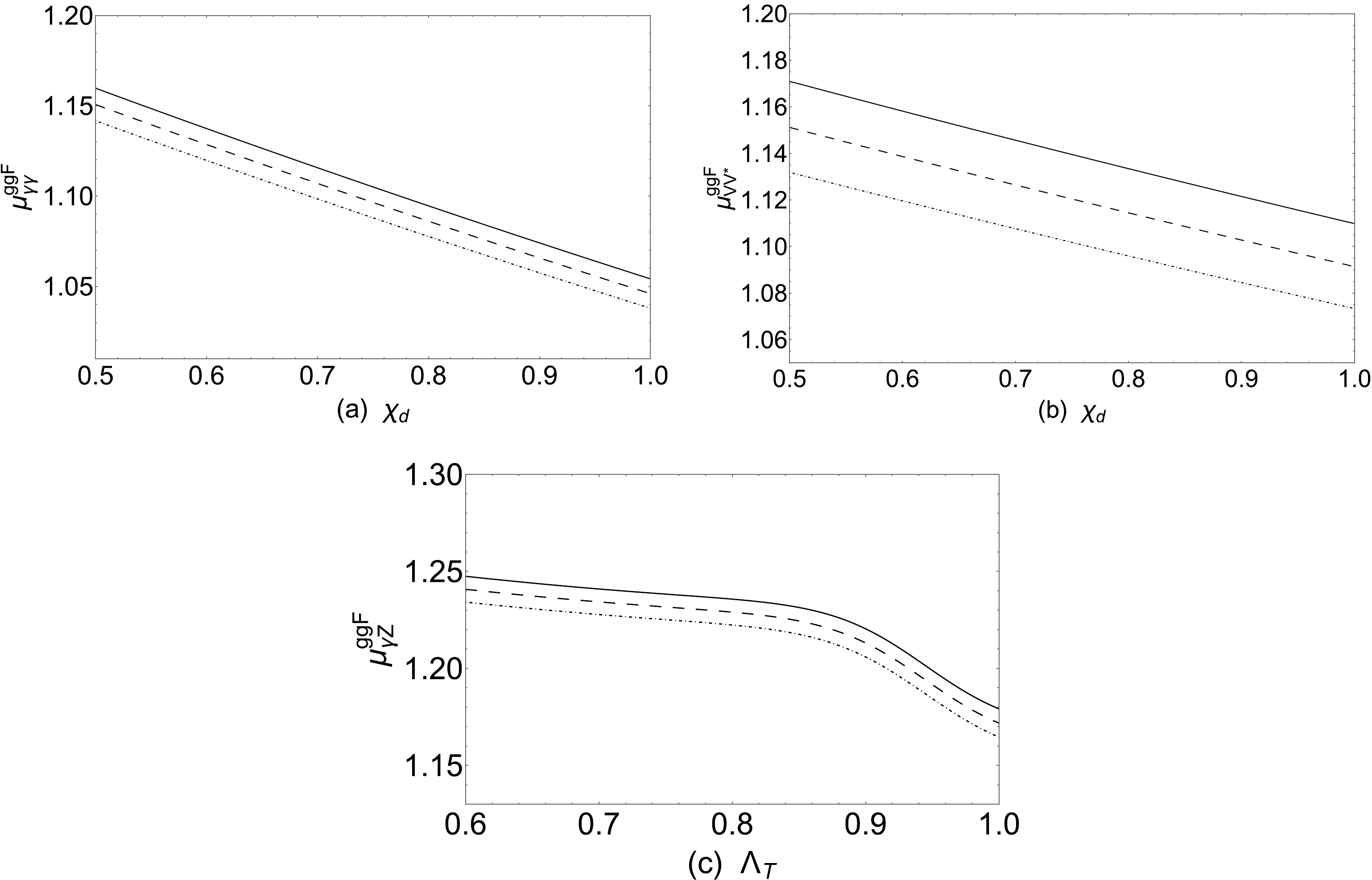
Figure 3. (a)
$ \mu_{\gamma\gamma}^{ggF} $ varing with$ \chi_d $ for$ T_{\chi_t}=-800\; {\rm{GeV}} $ (solid line),$ T_{\chi_t}=-900\; {\rm{GeV}} $ (dashed line), and$ T_{\chi_t}=-1000\; {\rm{GeV}} $ (dot dashed line). (b)$ \mu_{VV^*}^{ggF} $ varying with$ \chi_d $ for$ \Lambda_T=0.7 $ (solid line),$ \Lambda_T=0.8 $ (dashed line), and$ \Lambda_T=0.9 $ (dot dashed line). (c)$ \mu_{Z\gamma}^{ggF} $ varying with$ \Lambda_T $ for$ \chi_d=0.7 $ (solid line),$ \chi_d=0.8 $ (dashed line), and$ \chi_d=0.9 $ (dot dashed line).The signal strengths for the processes
$ h\rightarrow ZZ^* $ and$ h\rightarrow WW^* $ are very close. Therefore, we take$ \mu^{ggF}_{VV^*}=\mu^{ggF}_{WW^*}=\mu^{ggF}_{ZZ^*} $ for simplicity, and we only show the signal strength of$ h\rightarrow ZZ^* $ . We take the parameters$ M_2=1500\; {\rm{GeV}} $ ,$ T_{\chi_d}=-800\; {\rm{GeV}} $ ,$ T_{\chi_t}=-800\; {\rm{GeV}} $ , and$ A_t=1500\; {\rm{GeV}} $ , and we display the signal strength of$ h\rightarrow VV^* $ varying with$ \chi_d $ in Fig. 3(b) for$ \Lambda_T=0.7 $ (solid line),$ \Lambda_T=0.8 $ (dashed line), and$ \Lambda_T=0.9 $ (dot dashed line). In Fig. 3(b), the signal strength of$ h\rightarrow VV^* $ decreases with the increase in$ \chi_d $ . These curves are above 1.073 and below 1.171, and their behaviors are similar. The experiment constraints [3] are$\mu^{({\rm exp})}_{ZZ^*}=1.01\pm 0.07$ ,$\mu^{({\rm exp})}_{WW^*}=1.19\pm 0.12$ . Thus, our calculated result$ \mu^{ggF}_{ZZ^*} $ satisfies the experimental constraint where the error is$ 1\sigma $ , and$ \mu^{ggF}_{WW^*} $ satisfies the experimental constraint where the error is$ 2\sigma $ .The new physics contributions to the decay
$ h\rightarrow MZ $ come from the effective coupling of$ hZ\gamma $ . Therefore, we study the process$ h\rightarrow Z\gamma $ in this subsection. In the numerical calculation of the process$ h\rightarrow Z\gamma $ , we take the parameters$ M_2=1500\; {\rm{GeV}} $ ,$ T_{\chi_d}=-800\; {\rm{GeV}} $ ,$T_{\chi_t}=-800 {\rm{GeV}}$ , and$ A_t=1500\; {\rm{GeV}} $ . In Fig. 3(c), these curves are close to each other, and they vary from 1.164 to 1.248. When$ 0.6\leq \Lambda_T\leq 0.9 $ , all the lines have a smaller slope, and when$ 0.9\leq \Lambda_T\leq 1 $ , all the lines here have a larger slope. The result agrees with the observed signal strength with 1.5σ. -
In this subsection, we will study the processes
$ h\rightarrow MZ $ . The vector meson decay constants for ω, ρ, ϕ,$ J/\psi $ , and Υ can be found in Table 1. The NP contribution of the process$ h\rightarrow MZ $ comes from the effective coupling$ hZ\gamma $ . Thus, our calculated results of the$ h\rightarrow MZ $ decay for different mesons should be similar.Now, we study the signal strengths of the process
$ h\rightarrow MZ $ . First, we take the parameters$ T_{\chi_d}=-800\; {\rm{GeV}} $ ,$ T_{\chi_t}=-800\; {\rm{GeV}} $ , and$ A_t=1500\; {\rm{GeV}} $ . We depict the signal strengths of the$ h\rightarrow MZ $ processes in Fig. 4. In Fig. 4, the solid line is obtained with$ \chi_d=0.7 $ ,$ \Lambda_T=0.9 $ ; the dashed line is obtained with$ \chi_d=0.8 $ ,$ \Lambda_T=0.8 $ ; and the dot dashed line is obtained with$ \chi_d=0.9 $ ,$ \Lambda_T=0.7 $ . As can be observed from Fig. 4, the signal strengths increase with the increase in$ M_2 $ at$ 1000\; {{\rm{GeV}}} \leq M_2\leq 1100\; {\rm{GeV}} $ , and the signal strengths decrease with the increase in$ M_2 $ at$ 1100\; {{\rm{GeV}}}\leq M_2\leq 2000\; {\rm{GeV}} $ . The signal strengths of the$ h\rightarrow \omega Z $ processes are in the 1.18–1.223 region; the signal strengths of the$ h\rightarrow \rho Z $ processes are in the 1.183–1.235 region; the signal strengths of the$ h\rightarrow \phi Z $ processes are in the 1.141–1.172 region; the signal strengths of the$ h\rightarrow J\psi Z $ processes are in the 1.147– 1.179 region; and the signal strengths of the$ h\rightarrow \Upsilon Z $ processes are in the 1.108–1.138 region.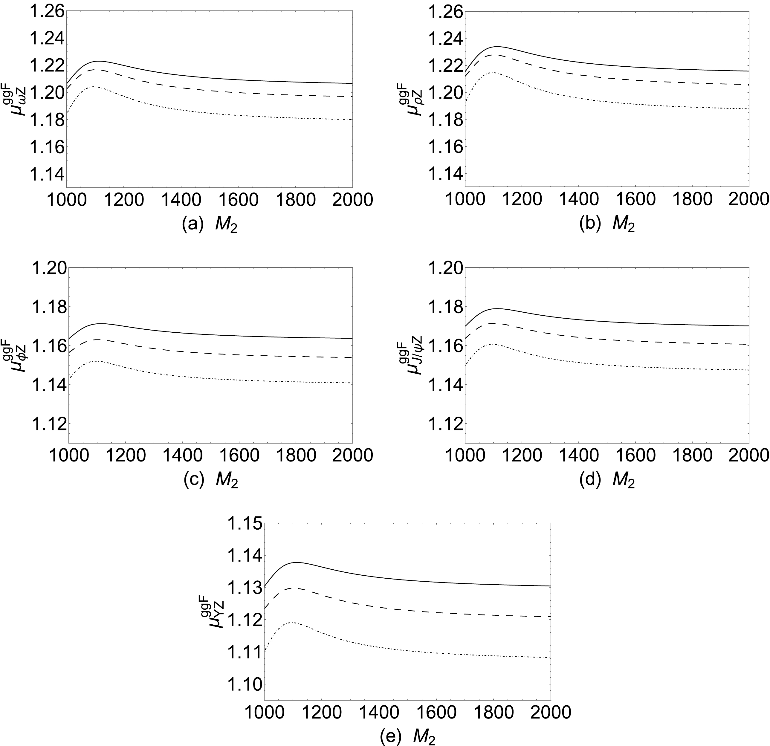
Figure 4. Signal strengths versus
$ M_2 $ for$ \chi_d=0.7 $ ,$ \Lambda_T=0.9 $ (solid line),$ \chi_d=0.8 $ ,$ \Lambda_T=0.8 $ (dashed line), and$ \chi_d=0.9 $ ,$ \Lambda_T=0.7 $ (dot dashed line).The new contributions to the
$ h\rightarrow MZ $ decay come from the effective coupling of$ h\gamma Z $ . Thus, we can infer that our results are consistent with the$ h\rightarrow \gamma Z $ process. As can be observed in Fig. 3(c), the parameter$ \Lambda_T $ has obvious influence on the signal strength$ \mu_{Z\gamma}^{ggF} $ . Thereore, we should research the signal strengths of the$ h\rightarrow MZ $ processes versus$ \Lambda_T $ . We take the parameters$ M_2=1500 $ GeV,$ T_{\chi_d}=-800\; {\rm{GeV}} $ ,$ T_{\chi_d}=-800\; {\rm{GeV}} $ , and$ A_t=1500 $ GeV. The Higgs mass should satisfy the$ 3\sigma $ error of the experimental constraints, and hence,$ \Lambda_T $ is changed from$ 0.6 $ to$ 1 $ with$ \chi_d=0.7,\; 0.8,\; 0.9 $ . The results for signal strengths of$ \mu^{ggF}_{MZ} $ versus$ \Lambda_T $ are plotted in Fig. 5. The$ \mu_{\omega Z}^{ggF} $ values are in the 1.133–1.238 region, the$ \mu_{\rho Z}^{ggF} $ values are in the 1.138–1.249 region, the$ \mu_{\phi_Z}^{ggF} $ values are in the 1.109–1.191 region, the$ \mu_{J/\psi Z}^{ggF} $ values are in the 1.112– 1.198 region, and the$ \mu_{\Upsilon Z}^{ggF} $ values are in the 1.07–1.155 region. It can be observed that the signal strengths of$ h\rightarrow MZ $ are similar to the signal strength of$ h\rightarrow Z\gamma $ . In Fig. 5, with solid lines, all the curves vary from 1.164 to 1.248. When$ 0.6\leq \Lambda_T\leq 0.9 $ , all the lines here have a smaller slope. When$ 0.9\leq \Lambda_T\leq 1 $ , all the lines here have a larger slope. As can be observed, the signal strengths of$ h\rightarrow MZ $ decrease as$ \chi_d $ increases.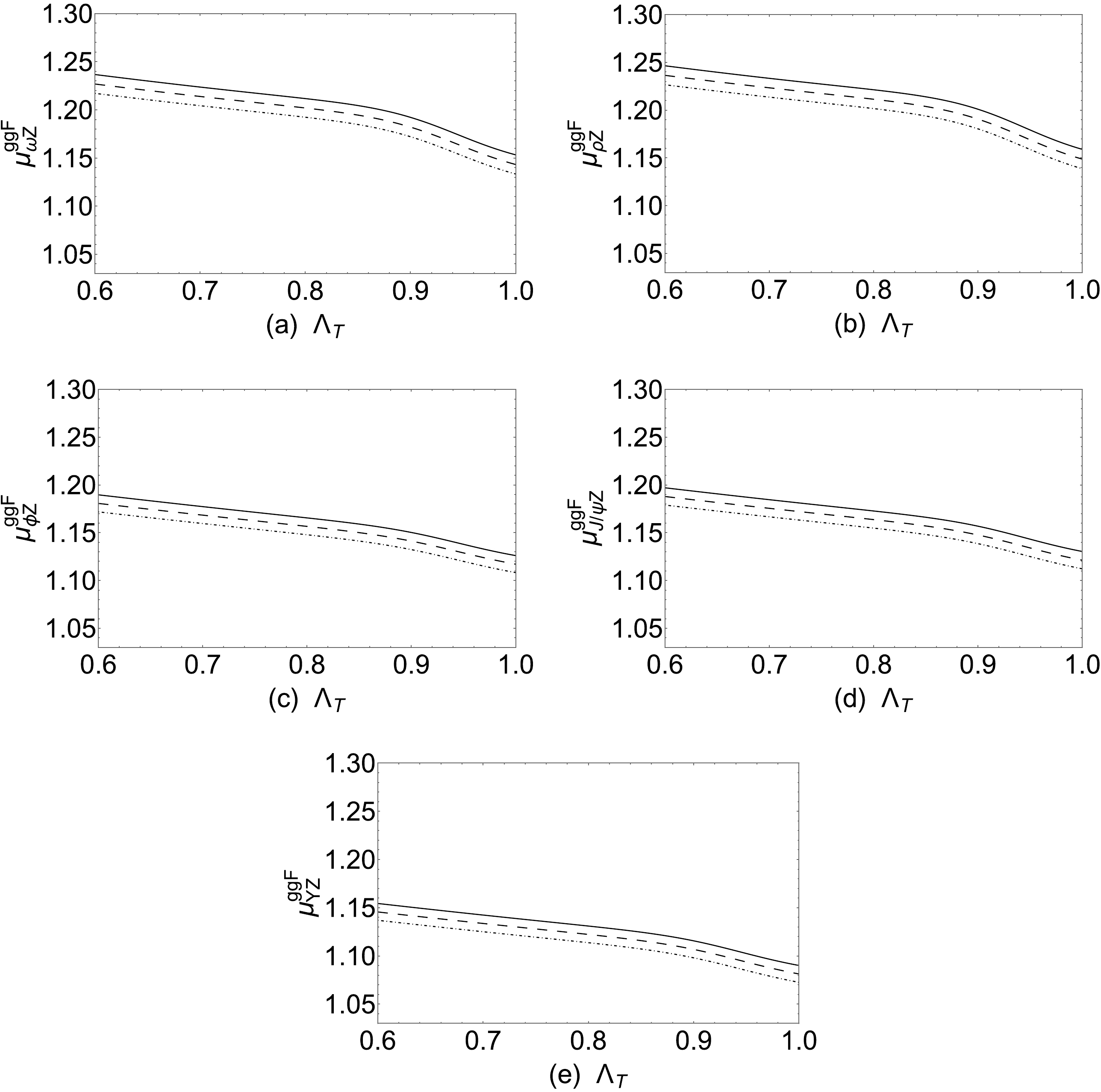
Figure 5. Signal strengths versus
$ \Lambda_T $ plotted with a solid line$ (\chi_d=0.7) $ , dashed line$ (\chi_d=0.8) $ , and dot dashed line$ (\chi_d=0.9) $ .We now study the effect of
$ T_{\chi_d} $ on the signal strengths of$ h\rightarrow MZ $ . We take the parameters$ M_2=1500\; {\rm{GeV}} $ ,$ \Lambda_T=0.8 $ ,$ \chi_d=0.7 $ , and$ T_{\chi_t}=-800\; {\rm{GeV}} $ . The SM-like Higgs mass should satisfy the$ 3\sigma $ error of the experimental constraints, and thus, we let$ T_{\chi_d} $ vary from$ -1000\; {\rm{GeV}} $ to$ 1000\; {\rm{GeV}} $ with$ A_t=1000, \; 1200,\; 1500\; {\rm{GeV}} $ . We plot the signal strengths of the$ h\rightarrow MZ $ processes in Fig. 6. In Fig. 6, the solid lines are obtained with$ A_t=1000\; {\rm{GeV}} $ , the dashed lines are obtained with$ A_t=1200\; {\rm{GeV}} $ , and the dot dashed lines are obtained with$ A_t=1500\; {\rm{GeV}} $ . In Fig. 6, we can see that the signal strengths increase with the increase in$ T_{\chi_d} $ . In Fig. 6(a) and Fig. 6(b), the signal strengths of the$ h\rightarrow \omega Z $ and$ h\rightarrow \rho Z $ processes are in the 1.181–1.227 and 1.19–1.237 regions, respectively. In Fig. 6(c) and Fig. 6(d), the signal strengths of the$ h\rightarrow \phi Z $ and$ h\rightarrow J/\psi Z $ processes are in the 1.138–1.178 and 1.145–1.186 regions, respectively. The meson Υ is the heaviest meson we have studied, and thus, the signal strength of the$ h\rightarrow \Upsilon Z $ process is obviously lower than the other results in Fig. 6. The signal strength of the$ h\rightarrow \Upsilon Z $ process is in the 1.105–1.142 region. We can see from Fig. 6 that$ A_t $ has a great influence on the signal strengths of$ h\rightarrow MZ $ . The signal strengths of$ h\rightarrow MZ $ increase as$ A_t $ increases.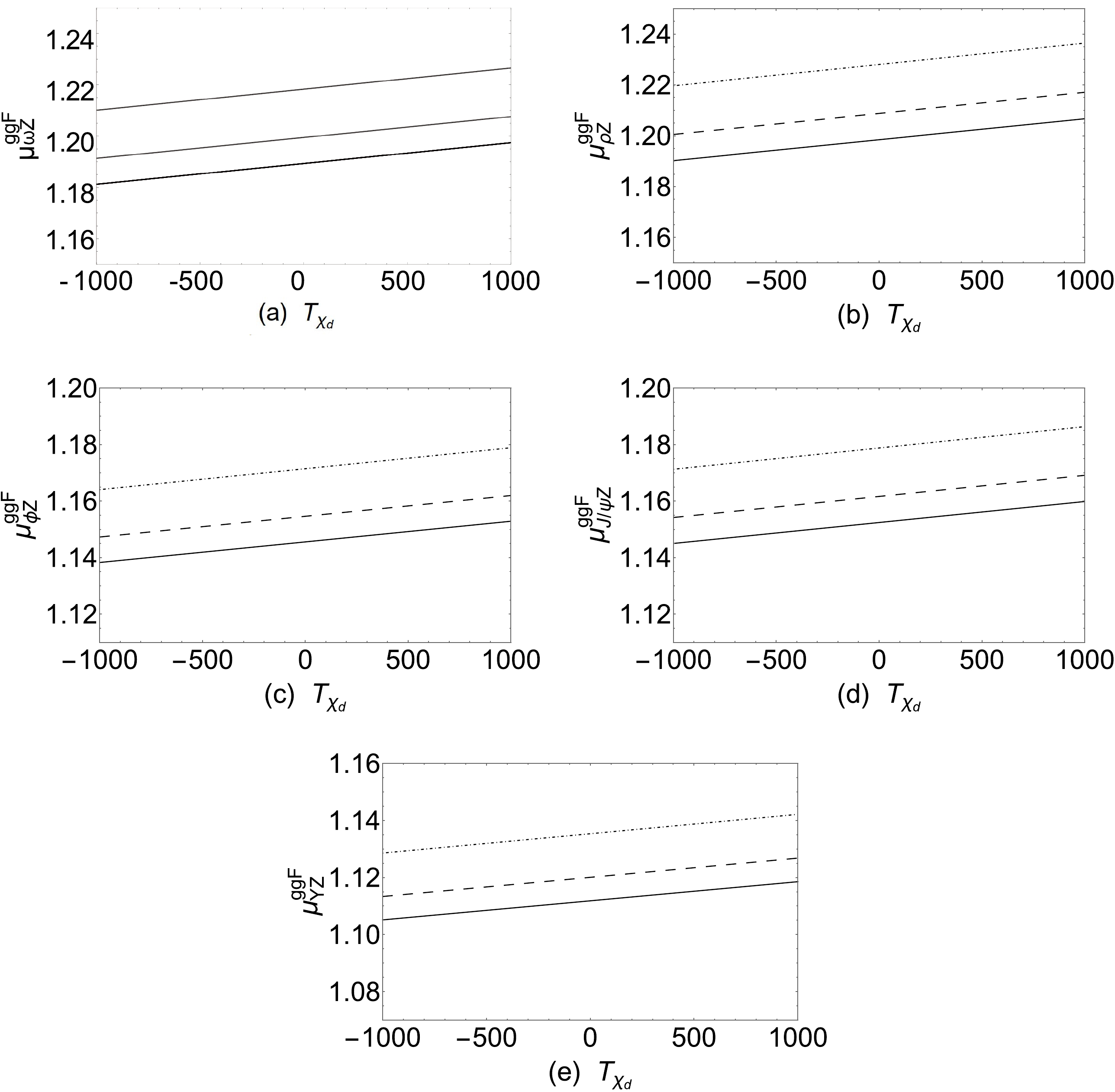
Figure 6. Signal strengths versus
$ T_{\chi_d} $ plotted for$ A_t=1000\; {\rm{GeV}} $ (solid line),$ A_t=1200\; {\rm{GeV}} $ (dashed line), and$ A_t=1500\; {\rm{GeV}} $ (dot dashed line).Finally, we study the effect of
$ A_t $ on the signal strengths of the$ h\rightarrow MZ $ processes. The coupling of Higgs and third generation squarks include$ A_t $ . We take the parameters$ M_2=1500\; {\rm{GeV}} $ ,$ T_{\chi_d}=-800\; {\rm{GeV}} $ , and$ T_{\chi_t}= -800\; {\rm{GeV}} $ . The SM-like Higgs mass should satisfy the$ 3\sigma $ error of the experimental constrains, and thus, we let$ A_t $ vary from$ -1000\; {\rm{GeV}} $ to$ 1000\; {\rm{GeV}} $ with$ (\Lambda_T=0.5, \chi_d=0.8) $ ,$ (\Lambda_T=0.6,\; \chi_d=0.7) $ , and$ (\Lambda_T=0.7,\; \chi_d=0.6) $ . We plot the signal strengths of the$ h\rightarrow MZ $ process in Fig. 7. In Fig. 7, the solid lines are obtained with$ \Lambda_T=0.5 $ ,$ \chi_d=0.8 $ , the dashed lines are obtained with$ \Lambda_T=0.6 $ ,$ \chi_d=0.7 $ , and the dot dashed lines are obtained with$ \Lambda_T=0.7 $ ,$ \chi_d=0.6 $ . In Fig. 7(a) and Fig. 7(b), the signal strengths of the$ h\rightarrow \omega Z $ and$ h\rightarrow \rho Z $ processes are in the 1.165–1.253 and 1.174–1.265 regions, respectively. The signal strengths of the$ h\rightarrow \phi Z $ and$ h\rightarrow J/\psi Z $ processes are in the 1.125–1.205 and 1.132–1.213 regions. For the heaviest meson Υ we have studied, the signal strength of$ h\rightarrow \Upsilon Z $ is obviously lower than the other results in Fig. 7. The lines in Fig. 7(e) are in the 1.095–1.169 region.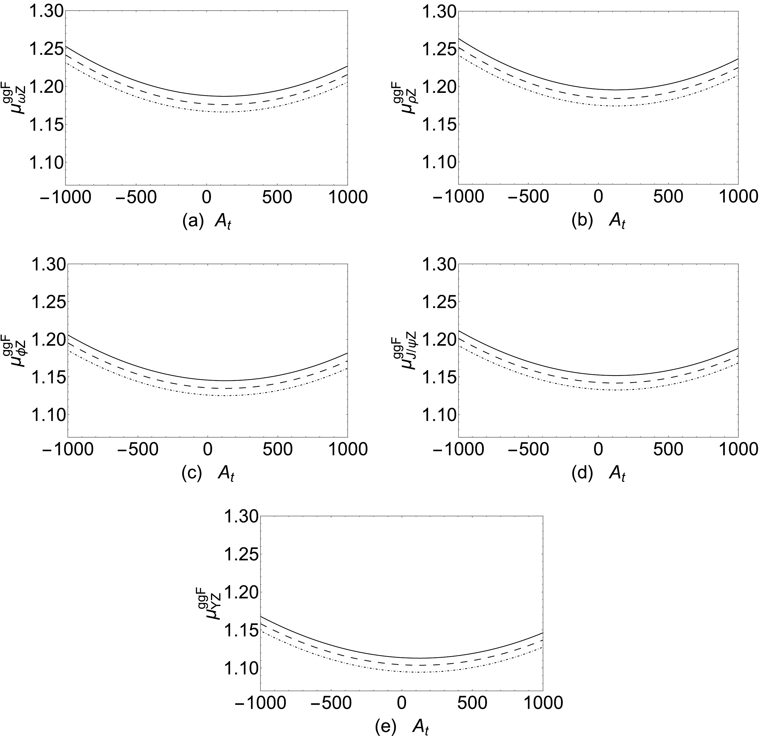
Figure 7. Signal strengths versus
$ A_t $ plotted for$ \Lambda_T=0.5 $ ,$ \chi_d=0.8 $ (solid line),$ \Lambda_T=0.6 $ ,$ \chi_d=0.7 $ (dashed line), and$ \Lambda_T=0.7 $ ,$ \chi_d=0.6 $ (dot dashed line). -
In this work, we study the decays
$ h\rightarrow \gamma Z $ and$ h\rightarrow MZ $ in the TNMSSM, with$ M=\omega,\rho,\phi,J/\psi,\Upsilon $ . The$ h\rightarrow MZ $ decay has two types of contributions: direct and indirect. For the indirect contributions, there is a process$ h\rightarrow Z\gamma^*\rightarrow MZ $ , where$ \gamma^* $ is off-shell and changes into the final state vector meson. No$ h\gamma Z $ coupling exists at the tree level, but it can be contributed by a loop diagram. In the models beyond the SM, the coupling constant can be divided into two parts: CP-even coupling constant$ C_{\gamma Z} $ and CP-odd coupling constant$ \tilde{C}_{\gamma Z} $ . The CP-even coupling constant$ C_{\gamma Z} $ is more important than the CP-odd coupling constant$ \tilde{C}_{\gamma Z} $ .The experiment results of the signal strengths
$ \mu^{ggF}_{\gamma\gamma} $ and$ \mu^{ggF}_{ZZ} $ are$ \mu^{ggF}_{\gamma\gamma}=1.10 \pm 0.07 $ and$ \mu^{ggF}_{ZZ}=1.01 \pm 0.07 $ . Our numerical results of the signal strengths$ \mu^{ggF}_{\gamma\gamma} $ and$ \mu^{ggF}_{ZZ} $ are in the 1.035–1.16 and 1.073–1.171 regions, which satisfy the error of$ 1\sigma $ . Our numerical results of the signal strength in the 1.164–1.248 region agree with the observed signal strength with 1.5σ. The numerical results show that the TNMSSM contributions to the$ h\rightarrow \omega Z $ and$ h\rightarrow \rho Z $ processes are more significant. The signal strengths$ \mu^{ggF}_{\omega Z,\rho Z} $ are approximately 1.13–1.26. The TNMSSM corrections to the$ h\rightarrow \phi Z $ and$ h\rightarrow J/\psi Z $ processes are 1.11–1.21, and to$ h\rightarrow \Upsilon Z $ they are approximately 1.07–1.17. The$ h\rightarrow MZ $ decays may be accessible at future high energy colliders. -
The form factors are
$ A_0(\tau,\lambda) =I_1(\tau,\lambda), $

(A1) $ A_{1/2}(\tau,\lambda) =I_1(\tau,\lambda)-I_2(\tau,\lambda) $

(A2) with
$ \begin{aligned}[b] I_1(\tau,\lambda)=\;&\frac{\tau\lambda}{2(\tau-\lambda)}+\frac{\tau^2 \lambda^2}{2(\tau-\lambda)^2}[f(\tau^{-1})-f(\lambda^{-1})]\\&+\frac{\tau^2\lambda}{(\tau-\lambda)^2}[g(\tau^{-1})-g(\lambda^{-1})], \end{aligned} $

(A3) $ I_2(\tau,\lambda)=-\frac{\tau \lambda}{2(\tau-\lambda)}[f(\tau^{-1})-f(\lambda^{-1})]. $

(A4) Here,
$ f(x) $ and$ g(x) $ are as follows:$ \begin{array}{*{20}{l}} f(x)=\left\{\begin{array}{ll} \arcsin ^{2} \sqrt{x}, & x \leq 1 \\ -\dfrac{1}{4}\left[\ln \dfrac{1+\sqrt{1-1 / x}}{1-\sqrt{1-1 / x}}-{\rm i} \pi\right]^{2}, & x>1 \end{array}\right. \end{array} $

(A5) $ \begin{array}{*{20}{l}} g(x)=\left\{\begin{array}{ll} \sqrt{x^{-1}-1}\arcsin \sqrt{x}, & x \ge 1 \\ \dfrac{\sqrt{1-x^{-1}}}{2}\left[\ln \dfrac{1+\sqrt{1-1 / x}}{1-\sqrt{1-1 / x}}-{\rm i} \pi\right], & x<1 \end{array}\right. \end{array} $

(A6) -
In the basis
$ (\phi_d,\phi_u,\phi_s,\phi_T,\phi_{\bar{T}}) $ , the definition of mass squared matrix for neutral Higgs is given by$ \begin{array}{*{20}{l}} m_h^2=\begin{pmatrix} m_{\phi_d \phi_d}&m_{\phi_u \phi_d}&m_{\phi_s \phi_d}&m_{\phi_T \phi_d}&m_{\phi_{\bar{T}} \phi_d}\\ m_{\phi_d \phi_u}&m_{\phi_u \phi_u}&m_{\phi_s \phi_u}&m_{\phi_T \phi_u}&m_{\phi_{\bar{T}} \phi_u}\\ m_{\phi_d \phi_s}&m_{\phi_u \phi_s}&m_{\phi_s \phi_s}&m_{\phi_T \phi_s}&m_{\phi_{\bar{T}} \phi_s}\\ m_{\phi_d \phi_T}&m_{\phi_u \phi_T}&m_{\phi_s \phi_T}&m_{\phi_T \phi_T}&m_{\phi_{\bar{T}} \phi_T}\\ m_{\phi_d \phi_{\bar{T}}}&m_{\phi_u \phi_{\bar{T}}}&m_{\phi_s \phi_{\bar{T}}}&m_{\phi_T \phi_{\bar{T}}}&m_{\phi_{\bar{T}} \phi_{\bar{T}}}\\ \end{pmatrix} \end{array} $

(B1) where
$ \begin{aligned}[b] m_{\phi_d \phi_d}=\;&m_{H_d}^2+\frac{1}{8}(g_1^2+g_2^2)(2v_{\bar{T}}^2-2v_T^2+3v_d^2-v_u^2)\\ &+\sqrt{2}v_T\Re(T_{\chi_d})+\frac{|\lambda|^2}{2}(v_s^2+v_u^2)\\&-v_s v_{\bar{T}} \Re(\chi_d \Lambda_T^*)+(3v_d^2+2v_T^2)|\chi_d|^2, \end{aligned} $

(B2) $ \begin{aligned}[b] m_{\phi_d \phi_u}=\;&-\frac{1}{4}(g_1^2+g_2^2)v_d v_u-\frac{1}{\sqrt{2}}v_s \Re(T_\lambda) \\&+\frac{1}{2}v_T v_{\bar{T}} \Re(\lambda\Lambda_T^*)+v_d v_u |\lambda|^2-v_s v_{\bar{T}}\Re(\chi_t \lambda^*)\\&-v_s v_T\Re(\chi_d \lambda^*)-\frac{1}{2}v_s^2\Re(\kappa\lambda^*), \end{aligned} $

(B3) $ \begin{aligned}[b] m_{\phi_u \phi_u}=\;&m_{H_u}^2-\frac{1}{8}(g_1^2+g_2^2)(2v_{\bar{T}}^2-2v_T^2-3v_u^2+v_d^2)\\ &+\sqrt{2}v_{\bar{T}}\Re(T_{\chi_t})+\frac{1}{2}(v_d^2+v_s^2)|\lambda|^2\\&-v_s v_T \Re(\chi_t \Lambda_T^*)+(2v_{\bar{T}}^2+3v_u^2)|\chi_t|^2, \end{aligned} $

(B4) $ \begin{aligned}[b] m_{\phi_d \phi_s}=\;&v_d v_s|\lambda|^2-\frac{1}{\sqrt{2}}v_u \Re(T_\lambda)-v_s v_u \Re(\kappa\lambda^*) \\& -v_T v_u \Re(\lambda\chi_d^*)-v_{\bar{T}}v_u \Re(\chi_t \lambda^*)-v_d v_{\bar{T}} \Re(\Lambda_T \chi_d^*), \end{aligned} $

(B5) $ \begin{aligned}[b] m_{\phi_u \phi_s}=\;&v_s v_u|\lambda|^2-\frac{1}{\sqrt{2}}v_d\Re(T_\lambda)-v_d v_s\Re(\lambda\kappa^*) \\& -v_T v_d\Re(\lambda\chi_d^*)-v_d v_{\bar{T}}\Re(\lambda\chi_t^*)-v_T v_u\Re(\chi_t \Lambda_T^*), \end{aligned} $

(B6) $ \begin{aligned}[b] m_{\phi_s \phi_s}=\;&m_S^2+\frac{|\Lambda_T|^2}{2}(v_T^2+v_{\bar{T}}^2)-v_T v_{\bar{T}}\Re(\kappa\Lambda_T^*)\\&+3v_s^2|\kappa|^2-v_d v_u\Re(\lambda\kappa^*)+\frac{1}{2}(v_d^2+v_u^2)|\lambda|^2,\\&+\sqrt{2}v_s\Re(T_\kappa), \end{aligned} $

(B7) $ \begin{aligned}[b] m_{\phi_d \phi_T}=\;&-\frac{1}{2}(g_1^2+g_2^2)v_d v_u+\frac{1}{2}v_u v_{\bar{T}}\Re(\lambda\Lambda_T^*)\\&-v_u v_s\Re(\lambda\chi_d^*)+4v_d v_T|\chi_d|^2+\sqrt{2}v_d\Re(T_{\chi_d}), \end{aligned} $

(B8) $ \begin{aligned}[b] m_{\phi_u \phi_T}=\;&\frac{1}{2}(g_1^2+g_2^2)v_d v_T-v_u v_s\Re(\Lambda_T\chi_t^*)\\&-v_d v_s\Re(\lambda\chi_d^*)+\frac{1}{2}v_d v_{\bar{T}}\Re(\lambda\Lambda_T^*), \end{aligned} $

(B9) $ \begin{aligned}[b] m_{\phi_s \phi_T}=\;&v_s v_T|\lambda|^2-\frac{1}{\sqrt{2}}v_{\bar{T}}\Re(T_\Lambda)- v_s v_{\bar{T}}\Re(\kappa\Lambda_T^*)\\&-v_d v_u \Re(\lambda\chi_d^*)-\frac{1}{2}v_u^2\Re(\chi_t\Lambda_T^*), \end{aligned} $

(B10) $ \begin{aligned}[b] m_{\phi_T,\phi_T}=\;&m_T^2-\frac{1}{4}(g_1^2+g_2^2)(2v_{\bar{T}}^2-6v_T^2-v_u^2+v_d^2)\\&+2v_d^2|\chi_d|^2 +\frac{1}{2}(v_s^2+v_{\bar{T}}^2)|\Lambda_T|^2, \end{aligned} $

(B11) $ \begin{aligned}[b] m_{\phi_d,\phi_{\bar{T}}}=\;&\frac{1}{2}(g_1^2+g_2^2)v_d v_{\bar{T}}+\frac{1}{2}v_T v_u \Re(\lambda\Lambda_T^*) \\& -v_d v_s \Re(\chi_d\Lambda_T^*)-v_s v_u\Re(\chi_t\lambda^*), \end{aligned} $

(B12) $ \begin{aligned}[b] m_{\phi_u,\phi_{\bar{T}}}=\;&-\frac{1}{2}(g_1^2+g_2^2)v_{\bar{T}}v_u+\sqrt{2}v_u\Re(T_{\chi_t}) \\&+\frac{1}{2}v_d v_T\Re(\lambda\Lambda_T^*)-v_d v_s \Re(\lambda\chi_t^*)+4v_{\bar{T}}v_u|\chi_t|^2, \end{aligned} $

(B13) $ \begin{aligned}[b] m_{\phi_s,\phi_{\bar{T}}}=\;&v_s v_{\bar{T}}|\Lambda_T|^2-\frac{1}{\sqrt{2}}v_T\Re(T_\Lambda) -v_s v_T\Re(\kappa\Lambda_T^*)\\&-\frac{1}{2}v_d^2\Re(\Lambda_T \chi_d^*)-v_d v_u\Re(\lambda\chi_t^*), \end{aligned} $

(B14) $ \begin{aligned}[b] m_{\phi_T,\phi_{\bar{T}}}=\;&-(g_1^2+g_2^2)v_T v_{\bar{T}}-\frac{1}{\sqrt{2}}v_s \Re(T_\Lambda) -\frac{1}{2}v_s^2 \Re(\kappa\Lambda_T^*)\\&+\frac{1}{2}v_d v_u \Re(\lambda\Lambda_T^*)+v_T v_{\bar{T}}|\Lambda_T|^2, \end{aligned} $

(B15) $ \begin{aligned}[b] m_{\phi_{\bar{T}},\phi_{\bar{T}}}=\;&m_{\bar{T}}^2+\frac{1}{4}(g_1^2+g_2^2)(v_d^2-v_u^2-2v_T^2+6v_{\bar{T}})\\&+ \frac{1}{2}(v_s^2+v_T^2)|\Lambda_T|^2+2v_u^2|\chi_t|^2. \end{aligned} $

(B16) This matrix is diagonalized by
$ Z^{\rm H} $ :$ \begin{array}{*{20}{l}} Z^{\rm H}m_h^2 Z^{\rm H,\dagger}=m_{2,h}^{\rm dia} \end{array} $

with
$ \begin{aligned}[b]& \phi_d=\sum\limits_j Z_{j1}^{\rm H} h_j,\; \; \phi_u=\sum\limits_j Z_{j2}^{\rm H} h_j,\; \; \phi_s=\sum\limits_j Z_{j3}^{\rm H} h_j,\\& \phi_T=\sum\limits_j Z_{j4}^{\rm H} h_j,\; \; \phi_{\bar{T}}=\sum\limits_j Z_{j5}^{\rm H}. \end{aligned} $

In the basis (
$ \tilde{W}^- $ ,$ \tilde{H}_d^- $ ,$ \tilde{T}^- $ ), ($ \tilde{W}^+ $ ,$ \tilde{H}_u^+ $ ,$ \tilde{T}^+ $ ), the definition of mass matrix for charginos is given by$ \begin{array}{*{20}{l}} m_{\tilde{\chi}^-}=\begin{pmatrix} M_2 & \dfrac{1}{\sqrt{2}}g_2 v_u & g_2 v_T\\ \dfrac{1}{\sqrt{2}}g_2 v_d & \dfrac{1}{\sqrt{2}} v_s \lambda & -v_d \chi_d\\ g_2 v_{\bar{T}} & -v_u \chi_t & \dfrac{1}{\sqrt{2}} \Lambda_T v_s \end{pmatrix} \end{array} $

(B17) This matrix is diagonalized by U and V
$ \begin{array}{*{20}{l}} U^*m_{\tilde{\chi}^-}V^{\dagger}=m_{\tilde{\chi}^-}^{dia} \end{array} $

with
$ \begin{array}{*{20}{l}} \tilde{W}^-=\sum\limits_j U^*_{j1}\lambda_j^-,\; \; \; \; \tilde{H}_d^-=\sum\limits_j U^*_{j2}\lambda_j^-,\; \; \; \; \tilde{T}^-=\sum\limits_j U^*_{j3}\lambda_j^-\\ \tilde{W}^+=\sum\limits_j V^*_{1j}\lambda_j^+,\; \; \; \; \tilde{H}_u^+=\sum\limits_j V^*_{2j}\lambda_j^+,\; \; \; \; \tilde{T}^+=\sum\limits_j V^*_{3j}\lambda_j^+ \end{array} $

-
The CP-even tree level part of the tadpole are given by
$ \begin{aligned}[b]\\[-10pt] \frac{\partial V}{\partial \phi_{d}} =\;& +\frac{1}{8} \Big(g_{1}^{2} + g_{2}^{2}\Big)v_d \Big(2 v_{\bar{T}}^{2} -2 v_{T}^{2} - v_{u}^{2} + v_{d}^{2}\Big)+\frac{1}{4} \Big(v_{\bar{T}} \Big(\Big(-2 v_d v_s \chi_d + v_T v_u \lambda \Big)\Lambda_T^*\\ &-2 v_s v_u \lambda \chi_t^* \Big)- v_{s}^{2} v_u \lambda \kappa^* +\Big(2 v_d \Big(v_{s}^{2} + v_{u}^{2}\Big)\lambda + v_u \Big(\Lambda_T v_T v_{\bar{T}} - v_s \Big(2 \Big(v_{\bar{T}} \chi_t + v_T \chi_d \Big) + v_s \kappa \Big)\Big)\Big)\lambda^*\\ & +4 v_d \Big(\sqrt{2} v_T {\Re\Big(T_{\chi_d}\Big)} + m_{H_d}^2\Big) -2 \Big(\sqrt{2} v_s v_u {\Re\Big(T_{\lambda}\Big)} + \Big(v_d \Big(-2 \Big(2 v_{T}^{2} + v_{d}^{2}\Big)\chi_d + \Lambda_T v_s v_{\bar{T}} \Big) + v_s v_T v_u \lambda \Big)\chi_d^* \Big)\Big) \end{aligned} $

(C1) $ \begin{aligned}[b] \frac{\partial V}{\partial \phi_{u}} =\;& +\frac{1}{8} \Big(g_{1}^{2} + g_{2}^{2}\Big)v_u \Big(-2 v_{\bar{T}}^{2} + 2 v_{T}^{2} - v_{d}^{2} + v_{u}^{2}\Big) +\frac{1}{4} \Big(\Big(4 v_{u}^{3} + 8 v_{\bar{T}}^{2} v_u \Big)|\chi_t|^2 +v_T \Big(-2 v_d v_s \lambda \chi_d^* + \Big(-2 v_s v_u \chi_t + v_d v_{\bar{T}} \lambda \Big)\Lambda_T^* \Big) \\ &+\Big(2 \Big(v_{d}^{2} + v_{s}^{2}\Big)v_u \lambda + v_d \Big(\Lambda_T v_T v_{\bar{T}} - v_s \Big(2 \Big(v_{\bar{T}} \chi_t + v_T \chi_d \Big) + v_s \kappa \Big)\Big)\Big)\lambda^* \\ &+v_u \Big(-2 \Lambda_T v_s v_T \chi_t^* + 4 \Big(\sqrt{2} v_{\bar{T}} {\Re\Big(T_{\chi_t}\Big)} + m_{H_u}^2\Big)\Big)\\ &+v_d \Big(-2 \sqrt{2} v_s {\Re\Big(T_{\lambda}\Big)} + \lambda \Big(-2 v_s v_{\bar{T}} \chi_t^* - v_{s}^{2} \kappa^* \Big)\Big)\Big) \end{aligned} $

(C2) $ \begin{aligned}[b] \frac{\partial V}{\partial \phi_s} =\;& \frac{1}{4} \Big(\Big(- v_{d}^{2} v_{\bar{T}} \chi_d + v_s \Big(2 \Lambda_T \Big(v_{T}^{2} + v_{\bar{T}}^{2}\Big) -2 v_T v_{\bar{T}} \kappa \Big) - v_T v_{u}^{2} \chi_t \Big)\Lambda_T^* +\Big(-2 v_d v_T v_u \lambda - \Lambda_T v_{d}^{2} v_{\bar{T}} \Big)\chi_d^* \\ &+\Big(-2 v_d v_{\bar{T}} v_u \lambda - \Lambda_T v_T v_{u}^{2} \Big)\chi_t^* +\Big(-2 v_d v_s v_u \lambda + 4 v_{s}^{3} \kappa \Big)\kappa^* +v_s \Big(-2 \Lambda_T v_T v_{\bar{T}} \kappa^* + 4 m_S^2 \Big) \\ &+2 \Big(- v_d v_u \Big(v_{\bar{T}} \chi_t + v_s \kappa + v_T \chi_d \Big) + v_s \Big(v_{d}^{2} + v_{u}^{2}\Big)\lambda \Big)\lambda^*\\ &+\sqrt{2} \Big(-2 v_d v_u {\Re\Big(T_{\lambda}\Big)} -2 v_T v_{\bar{T}} {\Re\Big(T_{\Lambda_T}\Big)} + v_{s}^{2} \Big(T_{\kappa}^* + T_{\kappa}\Big)\Big)\Big) \end{aligned} $

(C3) $ \begin{aligned}[b] \frac{\partial V}{\partial \phi_T} =\;& +\frac{1}{4} \Big(g_{1}^{2} + g_{2}^{2}\Big)v_T \Big(-2 v_{\bar{T}}^{2} + 2 v_{T}^{2} - v_{d}^{2} + v_{u}^{2}\Big) +\frac{1}{4} \Big(4 m_T^2 v_T +\Big(2 \Lambda_T v_T \Big(v_{s}^{2} + v_{\bar{T}}^{2}\Big) + v_d v_{\bar{T}} v_u \lambda - v_s \Big(v_s v_{\bar{T}} \kappa + v_{u}^{2} \chi_t \Big)\Big)\Lambda_T^* \\ &+\Lambda_T \Big(- v_{s}^{2} v_{\bar{T}} \kappa^* - v_s v_{u}^{2} \chi_t^* \Big)+v_d \Big(2 \Big(4 v_d v_T \chi_d - v_s v_u \lambda \Big)\chi_d^* + v_u \Big(-2 v_s \chi_d + \Lambda_T v_{\bar{T}} \Big)\lambda^* \Big) \\ &-2 \sqrt{2} v_s v_{\bar{T}} {\Re\Big(T_{\Lambda_T}\Big)} +2 \sqrt{2} v_{d}^{2} {\Re\Big(T_{\chi_d}\Big)} \Big) \end{aligned} $

(C4) $ \begin{aligned}[b] \frac{\partial V}{\partial \phi_{\bar{T}}} =\;& +\frac{1}{4} \Big(g_{1}^{2} + g_{2}^{2}\Big)v_{\bar{T}} \Big(2 v_{\bar{T}}^{2} -2 v_{T}^{2} - v_{u}^{2} + v_{d}^{2}\Big) +\frac{1}{4} \Big(4 v_{\bar{T}} \Big(2 v_{u}^{2} |\chi_t|^2 + m_{\bar{T}}^2\Big)\\ &+\Big(2 \Lambda_T \Big(v_{s}^{2} + v_{T}^{2}\Big)v_{\bar{T}} + v_d v_T v_u \lambda - v_s \Big(v_{d}^{2} \chi_d + v_s v_T \kappa \Big)\Big)\Lambda_T^* - \Lambda_T v_{s}^{2} v_T \kappa^* +v_d v_u \Big(-2 v_s \chi_t + \Lambda_T v_T \Big)\lambda^* \\ &+v_s \Big(-2 \Big(\sqrt{2} v_T {\Re\Big(T_{\Lambda_T}\Big)} + v_d v_u \lambda \chi_t^* \Big) - \Lambda_T v_{d}^{2} \chi_d^* \Big) +\sqrt{2} v_{u}^{2} \Big(T_{{\chi,t}^*} + T_{\chi_t}\Big)\Big) \end{aligned} $

(C5) Then, we can identify the
$ m_{H_d}^2 $ ,$ m_{H_u}^2 $ ,$ m_S^2 $ ,$ m_T^2 $ , and$ m_{\bar{T}}^2 $ by the minimum conditions of the scalar potential.Here, we show some corresponding vertexes in this model. Their concrete forms are shown as
$ C^L_{Z\chi^+_i\chi^-_j}= \frac{1}{2}\big(-2g_1\sin\theta_WU^*_{j3}U_{i3}+2g_2\cos\theta_WU^*_{j1}U_{i1}+(-g_1\sin\theta_W+g_2\cos\theta_W)U^*_{j2}U_{i2}\big) $

(C6) $ C^R_{Z\chi^+_i\chi^-_j}= \frac{1}{2}\big(-2g_1\sin\theta_WV^*_{j3}V_{i3}+2g_2\cos\theta_WV^*_{j1}V_{i1}+(-g_1\sin\theta_W+g_2\cos\theta_W)V^*_{j2}V_{i2}\big) $

(C7) $ C^L_{Z\chi^{++}\chi^{-}}= C^R_{h\chi^{++}\chi^{-}}=\big(-g_1\sin\theta_W+g_2\cos\theta_W\big) $

(C8) $ \begin{aligned}[b] C^L_{h_k\chi^+_i\chi^-_j}=\;& -\frac{1}{2}\big[g_2U^*_{j1}(2V^*_{i3}Z^H_{k4}+\sqrt{2}V^*_{i2}Z^H_{k2})+U^*_{j2}(-2\chi_d V^*_{i3}Z^H_{k1}+\sqrt{2}g_2V^*_{i1}Z^H_{k3}+\sqrt{2}\lambda V^*_{i2}Z^H_{k3})\\ & +U^*_{j3}(-2\chi_tV^*_{i2}Z^H_{k2}+2g_2V^*_{i1}Z^H_{k5}+\sqrt{2}\Lambda_TV^*_{i3}Z^H_{k3})\big] \end{aligned} $

(C9) $ \begin{aligned}[b] C^R_{h_k\chi^+_i\chi^-_j}=\;& -\frac{1}{2}\big[g_2U_{i1}(2V_{j3}Z^H_{k4}+\sqrt{2}V_{j2}Z^H_{k2})+U_{i2}(-2\chi_d^* V_{j3}Z^H_{k1}+\sqrt{2}g_2V_{j1}Z^H_{k3}+\sqrt{2}\lambda^* V_{j2}Z^H_{k3})\\ & +U_{i3}(-2\chi_t^*V_{j2}Z^H_{k2}+2g_2V_{j1}Z^H_{k5}+\sqrt{2}\Lambda_T^*V_{j3}Z^H_{k3})\big] \end{aligned} $

(C10) $ C^L_{h_k\chi^{++}\chi^{-}}= \frac{1}{\sqrt{2}}\Lambda_T Z^H_{k3} $

(C11) $ C^R_{h_k\chi^{++}\chi^{-}}= \frac{1}{\sqrt{2}}\Lambda_T^* Z^H_{k3} $

(C12) As the coupling between Higgs particles and charged scalar particles is very complicated, we calculate it by computer.
$ \begin{aligned}[b] V_{\rm scalar}=\;& W^*_iW^i+\frac{1}{2}\sum\limits_{a}g_2^2\big[H_u^\dagger\frac{\sigma^a}{2}H_u+H_d^\dagger\frac{\sigma^a}{2}H_d+Tr(T^\dagger\sigma^a T)+Tr(\bar{T}^\dagger\sigma^a \bar{T})\big]^2 g^2_1\Bigg[\frac{1}{2}H_u^\dagger H_u-\frac{1}{2}H_d^\dagger H_d+T^\dagger T\\&-\bar{T}^\dagger\bar{T}+\frac{1}{6}\tilde{Q}^\dagger\tilde{Q}-\frac{1}{2}\tilde{L}^\dagger\tilde{L} -\frac{2}{3}\tilde{u}^*_R\tilde{u}_R+\frac{1}{3}\tilde{d}^*_R\tilde{d}_R+\tilde{e}^*_R\tilde{e}_R+Tr(T^\dagger T)-Tr(\tilde{T}^\dagger\tilde{T})\Bigg]^2+V_{\rm soft} \end{aligned} $

where
$ W_i=\dfrac{\partial W}{\partial\phi_i} $ . The coefficient C is as follows:$ C_{h_k\phi_i\phi_j}=\frac{\partial^3 V_{\rm scalar}}{\partial h_k\partial \phi_i\partial\phi_j}\bigg|_{<H^0_{d,u}>=\frac{v_{d,u}}{\sqrt{2}},<S>=\frac{v_s}{\sqrt{2}},<T>=\frac{v_T}{\sqrt{2}},<\bar{T}>=\frac{v_{\bar T}}{\sqrt{2}},<\rm the\; other \; fields>=0}\\ $

(58) where
$ \phi_i $ represents the scalar field:$ H^{\pm} $ ,$ H^{\pm\pm} $ ,$ \tilde{u}_L $ ,$ \tilde{u}_R $ ,$ \tilde{d}_L $ ,$ \tilde{d}_R $ ,$ \tilde{e}_L $ , and$ \tilde{e}_R $ .
Higgs boson decays h→MZ in the TNMSSM
- Received Date: 2024-03-02
- Available Online: 2024-09-15
Abstract: We study the SM-like Higgs boson decays


 DownLoad: