-
Heavy-ion collision experiments at intermediate and high energies have recently become a key tool for studying the microscopic structure of matter and exploring the physical laws of the universe under extreme conditions. These collision processes reveal the mysteries of strong interactions and provide a unique experimental platform to simulate and explain the evolutionary state of matter in the early stages after the Big Bang [1]. In addition, understanding the interaction mechanisms of intermediate and high energy heavy-ion collisions holds significant scientific value in assessing radiation damage to spacecraft equipment, studying the propagation of heavy ions in Galactic Cosmic Rays (GCR) in the interstellar medium, and understanding the composition of cosmic rays and the biological effects of radiation [2]. In physics, heavy ions lose energy significantly when they come to a near stop in the medium, a phenomenon known as the Bragg effect. In biology, the dose required to kill tumor cells at the same rate is much smaller than that of conventional radiation [3].
Cosmic ray particles are mainly composed of protons (p), accounting for about 87%, followed by helium (He), accounting for about 12%, and the remaining 1% are heavy ions. The energies of these particles can range from a few tens of A MeV to more than 1015 A MeV. Although heavy ions, such as C, Ne, Si, Fe, are much less abundant than p and He, they are the main components that cause biological effects [4]. Silicon is also one of the relatively abundant heavy elements in galactic cosmic rays and is a main fragmentation product of the interaction of Fe and other heavy particles. In addition, elemental silicon is a component of electronic equipment materials for manned space vehicles and the International Space Station. Therefore, the study of intermediate and high energy
$ ^{28} {\rm{Si}}$ fragmentation is of great scientific value in medical radiation therapy, human radiation protection in the space environment, and aerospace electronic equipment materials research.Recent studies on intermediate and high energy heavy-ion collisions have focused on heavy-ion fragmentation cross sections, which consist mainly of the total charge-change and fragment production cross sections. An accurate database of heavy-ion fragmentation cross sections is an important tool for developing theoretical models. However, conducting an entire experimental program covering all projectiles and targets over the large range of energies required is impractical. Therefore, attempting to use existing cross-section databases to continuously create and refine the corresponding theoretical models to reproduce and predict nuclear data is necessary.
Theoretically, the total charge-changing cross sections are predominantly simulated using established models, such as the NUCFRG2 model [5], the PHITS code system [6], and the Bradt-Peters semi-empirical formula [7]. Empirical parameter models have been widely used to simulate and predict fragment production cross sections. Among them, the Cummings model [8, 9], the Nilsen model [10], EPAX2 [11], modified EPAX2 [12], EPAX3 [13, 14], and the FRACS model [15] have been commonly used. Experimentally, different groups worldwide have utilized various measurement methods to investigate the total charge-change and fragment production cross sections of an
$ ^{28} {\rm{Si}}$ projectile interacting with different targets [16−30]. Detailed studies can be found in these references [16−30], which contain almost all current research results on the fragmentation cross section of the$ ^{28} {\rm{Si}}$ projectile. However, some discrepancies exist in the fragmentation cross section data for the$ ^{28} {\rm{Si}}$ projectile interacting with different targets, both between experiments and in theoretical-experimental comparisons. These discrepancies require urgent attention, and a systematic and comprehensive study of the reaction mechanisms is needed to address these issues.Machine learning (ML) has recently become an effective tool for processing complex big data owing to its powerful fitting and prediction capabilities and its high computational speed. For complex nonlinear systems, which are difficult or even impossible to solve with traditional models, machine learning has a strong feature extraction ability [31]. Machine learning is rapidly being integrated into physics, which has led to the gradual realization that machine learning is expected to form a new method of evaluating nuclear data and provide a novel research idea. In particular, the Bayesian neural network (BNN) method in machine learning, known for its strong predictive ability and capacity to provide theoretical error estimates for predicted values, has attracted the attention of many fields including nuclear physics.
Nowadays, machine learning methods, especially the BNN method, have been successfully applied to the study of many fundamental problems in nuclear physics. For example, in nuclear mass studies, Utama et al. [32] and Niu et al. [33] used the BNN method to improve the nuclear mass prediction of various models. Gao et al. [34] used a highly efficient machine learning algorithm to predict the masses of unknown nuclei. For a heavy-ion collision temperature study, Song et al. [35] proposed that the charge multiplicity distribution can be used as a thermometer for heavy ion collisions by linking the charge multiplicity distribution to the temperature of a de-exciting nucleus using a deep neural network (DNN). For the charge radii study, Dong et al. [36] introduced a novel method integrating a three-parameter formula with a BNN, effectively modeling the charge radii of nuclei with A
$ \geq $ 40 and Z$ \geq $ 20. The charge radii of the calcium isotopic chain are reproduced very well, including the parabolic behavior and strong odd-even staggerings. Utama et al. [37] used the proton number Z and mass number A of the nucleus as the inputs for training the BNN to achieve a relatively good description of the charge radius. However, the BNN method cannot describe odd-even staggerings, especially for calcium isotopes. For a β-decay half-lives study, Niu et al. [38] introduced an approach for the accurate prediction of β-decay half-lives using an ML method based on BNNs. The results reproduced the experimental data better with high accuracy and further provided a reasonable uncertainty evaluation for half-life prediction. For a nuclear fission yields study, Wang et al. [39] demonstrated that the BNN was particularly useful for evaluating fission yields when experimental data were incomplete. The results of the BNN evaluation were satisfactory in terms of the location of the distribution of fission yields and the energy dependence. For the charge yields of the fission fragments study, Qiao et al. [40] applied a BNN approach to learn the existing evaluated charge yields and infer the incomplete charge yields of$ ^{239} $ U. They found that a two-layer BNN was superior to a single-layer BNN in terms of overall performance. For a spallation reaction cross sections study, Ma et al. [41] demonstrated that the BNN method can provide good predictions of the residue fragment cross-sections in spallation reactions. Li et al. [42] used three algorithms commonly used in machine learning, artificial neural networks (ANN), convolutional neural networks (CNN), and light gradient boosting machine (LightGBM), to determine impact parameters by analyzing the features. The trained machine learning algorithm has good universality and can be used reliably for reconstructing impact parameters in experiments.This study uses the BNN method to directly learn the existing fragmentation cross sections of
$ ^{28} {\rm{Si}}$ projectiles and make predictions. Concurrently, the prediction ability of the BNN is analyzed by comparing the results with the experimental data and the prediction results of other theoretical models to provide a reference for the direct study of fragment cross sections using the BNN method. -
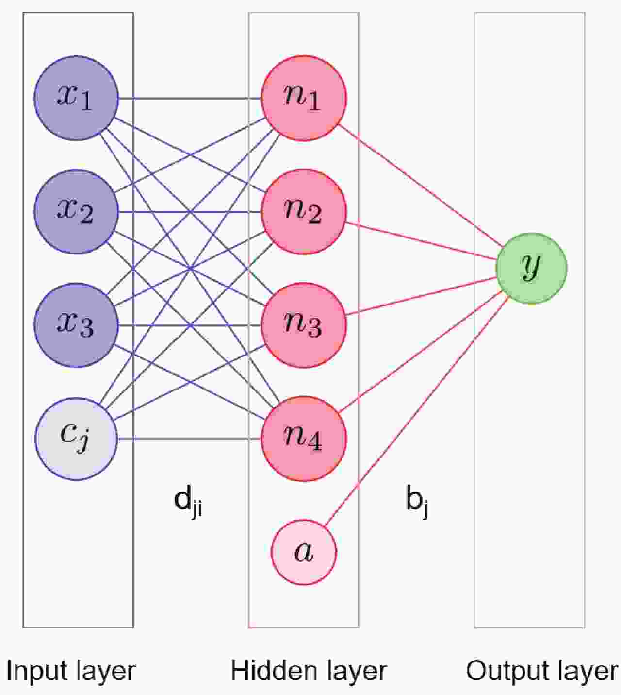
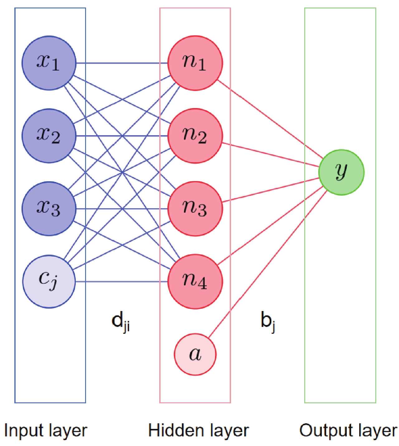
Bayesian neural networks (BNN) differ from other neural networks in that their weight parameters are random variables rather than definite values. That is, in a Bayesian neural network, parameters like weights and biases are no longer a definite value but become a distribution. The network structure of the BNN model mainly comprises an input layer, a hidden layer, and an output layer, with the input layer being a set of real input variables
$ x_{i} $ , and the output value$ y(x) $ can be calculated through the hidden layer. Figure 1 shows the schematic structure of a Bayesian neural network with one hidden layer. The function of the Bayesian neural network can be expressed as$ Y(x_{i},\theta) = a + \sum\limits_{j = 1}^{H} b_{j}f\left(c_{j} + \sum\limits_{i = 1}^{I} d_{ji}x_{i} \right) . $

(1) Here, H is the number of neurons in the hidden layer, I is the number of input variables, i represents the input unit, and j represents the hidden unit. a and
$ c_{j} $ are biases,$ b_{j} $ and$ d_{ji} $ are connection weights, which together form the parameters θ of the neural network, i.e.,$ \theta = \left\lbrace a, b_{j}, c_{j}, d_{ji} \right\rbrace $ . f is the activation function, which can be set to different types.The process of optimization and determination of the BNN model requires continuous learning from the dataset
$ D = \left\lbrace(x_{1},y_{1}),(x_{2},y_{2}),\cdots,(x_{n},y_{n}) \right\rbrace $ to determine the various parameters θ. Concurrently, the number of variables in the input layer, the number of layers in the hidden layer, the number of neurons in the hidden layer, and the number of outputs in the output layer can also be set.The Bayesian neural network method is based on the Bayesian theorem in mathematics, which aims to obtain the posterior probability distribution
$ P\left( \theta\mid D\right) $ of the parameters θ through training on the dataset$ D = \left\lbrace(x_{1},y_{1}), (x_{2},y_{2}),\cdots,(x_{n},y_{n}) \right\rbrace $ , and subsequently using it to predict new inputs. It can be written as$ P(\theta\mid D) = \frac{P(D\mid\theta)P(\theta)}{P(D)} \propto P(D\mid\theta)P(\theta). $

(2) Here,
$ P(\theta) $ is the prior probability distribution.$ P\left( D\mid\theta\right) $ is the likelihood function, which can be expressed as$ P\left( D\mid\theta\right) = \exp(-\chi^{2}/2) $ .$ P(D) $ is the normalization factor to ensure that the integral of the posterior probability is 1.We can make predictions based on the posterior distribution when we input the new data
$x_{\rm new}$ . The formula can be expressed as$ \langle Y_{\rm new}\rangle = \int Y(x_{\rm new},\theta)P(\theta\mid D) \mathrm{d}\theta . $

(3) In this study, 95% confidence intervals (CI) for quantification of uncertainty are given. More details about BNN can be found in Ref. [43].
-
In this study, the BNN neural network structure is defined as six inputs, i.e.,
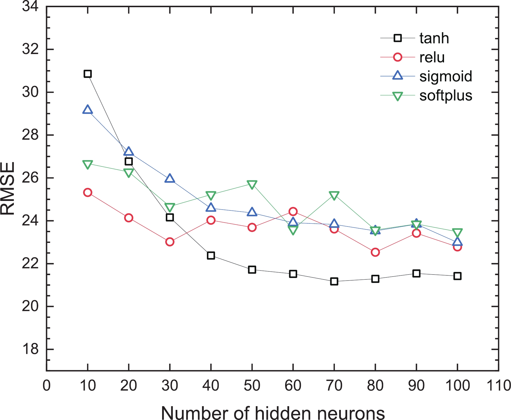
$ x_{i} = \left\lbrace A_{p}, Z_{p}, A_{t}, Z_{t}, Z_{f}, E \right\rbrace $ , which represent the mass number of the projectile, proton number of the projectile, mass number of the target nucleus, proton number of the target nucleus, proton number of the fragment, and incident energy of the projectile, respectively. The hidden layer is a single layer, and the output is the cross-section (mb) data.Table 1 presents the available data sets selected for our study. We use cross-validation to optimize the selection of activation functions and the number of neurons in the hidden layer. We repeat the ten-fold cross-validation process ten times, with each validation used to calculate the root mean square error (RMSE) of the predicted data. After ten iterations are completed, we calculate the mean value of the RMSE.
Reaction type E/(A MeV) $Z_{f}$ range

$^{28}{\rm{Si}}$ + H

263 350 467 503 6–13 560 765 770 1147 6–13 1296 14500 6–13 $^{28}{\rm{Si}}$ + C

218 266 268 344 6–13 467 503 560 723 6–13 736 765 770 788 6–13 1147 1296 14500 6–13 $^{28}{\rm{Si}}$ + Al

269 355 453 560 6–13 765 1160 14500 6–13 $^{28}{\rm{Si}}$ + Cu

273 344 442 545 6–13 765 1150 14500 6–13 $^{28}{\rm{Si}}$ + Ag

436 14500 6–13 $^{28}{\rm{Si}}$ + Sn

278 359 560 6–13 771 1155 6–13 $^{28}{\rm{Si}}$ + Pb

274 364 430 540 6–13 770 1145 14500 6–13 $^{28}{\rm{Si}}$ + CH2

600 788 1000 6–13 In this study, we conduct a comparative analysis for four commonly used activation functions, which are tanh, relu, sigmoid, and softplus. These activation functions play a central role in neural networks and affect the training efficiency and performance of the networks. Moreover, we consider the effect of different neurons in a single hidden layer. Figure 2 shows the mean value of the RMSE for predicted data in different activation functions. From the results in Fig. 2, the number of hidden neurons increases; the tanh function shows the optimal performance among the four activation functions, so we choose tanh as the activation function in this study. Further observation of Fig. 2 reveals that the mean value of the RMSE for the tanh activation function first decreased significantly and then stabilized, indicating a hidden neuron number that enables the RMSE to reach a minimum. In training, we finally determined that the optimal number of neurons is 70.
-
After determining the optimal network structure, we first divide the data in Table 1 into two parts: one part as the training set (T) and the other as the validation set (V). The training set (T) and the validation set (V) are randomly grouped and divided several times based on different energies and targets to verify the reliability of the prediction results of the BNN model, as shown in detail in Table 2. Then, we use the training set data to train the neural network and predict the validation set. The prediction results of the BNN are compared and analyzed with the existing experimental data and the prediction results of the Cummings old (shown as Cummings Old [1990] in figures), Cummings new (shown as Cummings New [1995] in figures), Nilsen (shown as Nilsen [1995] in figures), EPAX2 (shown as Sümmerer [2000] in figures), EPAX3 (shown as Sümmerer [2012] in figures), and FRACS (shown as Mei [2017] in figures) theoretical prediction models. Finally, the RMSEs between the predicted value of the different models and the experimental value are calculated to evaluate the model accuracy.
Group Validation set (V) Training set (T) 1 $^{28}{\rm{Si}}$ + H (467 A MeV)

Remaining data 2 $^{28}{\rm{Si}}$ + H (1296 A MeV)

Remaining data 3 $^{28}{\rm{Si}}$ + C (268 + 723 A MeV)

Remaining data 4 $^{28}{\rm{Si}}$ + Al (355 A MeV)

Remaining data 5 $^{28}{\rm{Si}}$ + Al (1160 A MeV)

Remaining data 6 $^{28}{\rm{Si}}$ + Cu (442 A MeV)

Remaining data 7 $^{28}{\rm{Si}}$ + Cu (545 A MeV)

Remaining data 8 $^{28}{\rm{Si}}$ + Ag (436 + 14500 A MeV)

Remaining data 9 $^{28}{\rm{Si}}$ + Sn (278 A MeV)

Remaining data 10 $^{28}{\rm{Si}}$ + Sn (771 A MeV)

Remaining data 11 $^{28}{\rm{Si}}$ + Pb (430 A MeV)

Remaining data 12 $^{28}{\rm{Si}}$ + Pb (1145 A MeV)

Remaining data 13 $^{28}{\rm{Si}}$ + CH2 (600 + 788 + 1000 A MeV)

Remaining data Table 2. Grouping setup of the training and validation sets.
Figures 3−10 show the predicted values of the BNN method and other theoretical models for each group of validation sets listed in Table 2, and compare the predicted values with the experimental values. The predicted values for the individual theoretical models in the figure are not depicted because the reaction type is beyond the range that the model can predict. As can be seen from Figs. 3−10, the predicted result reproduced by the BNN method is very close to the experimental value or even completely agrees with the experimental value within a 95% confidence interval. However, the predicted value of other theoretical models generally decreases as fragment charge Z decreases, with some deviations between the predicted result and the experimental value, which do not satisfactorily reproduce the experimental values. For example, the EPAX2 (Sümmerer [2000]) model generally underestimates the experimental values. When the charge number Z of the fragment is less than 9, the other six theoretical models generally tend to underestimate the experimental values. When Z is more than 9, the EPAX3 (Sümmerer [2012]) and FRACS (Mei [2017]) models generally tend to overestimate the experimental values, while the Cummings Old, Cummings New, and Nilsen models show a smooth curve that is relatively close to the experimental value; however, they do not show the odd-even staggering effect. In addition, the experimental value for the fragment production cross section at Z = 9 is lower, which is consistent with the findings of Ref. [22]. This may be because the charge number of the projectile fragment (Z = 9) is odd, resulting in a smaller production cross section compared to projectile fragments with even charge numbers (Z = 8) and (Z = 10). Notably, the data feature at Z = 9 is not reflected in the other six theoretical models, and only the BNN method successfully reproduces this feature.
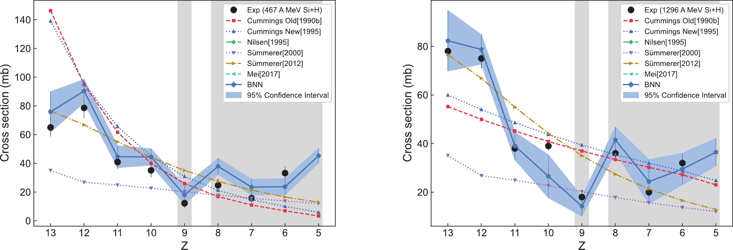
Figure 3. (color online) Predictions of the BNN method for the fragment production cross sections of
$ ^{28} {\rm{Si}}$ +H (467 A MeV) and$ ^{28} {\rm{Si}}$ +H (1296 A MeV), along with comparisons with other theoretical models.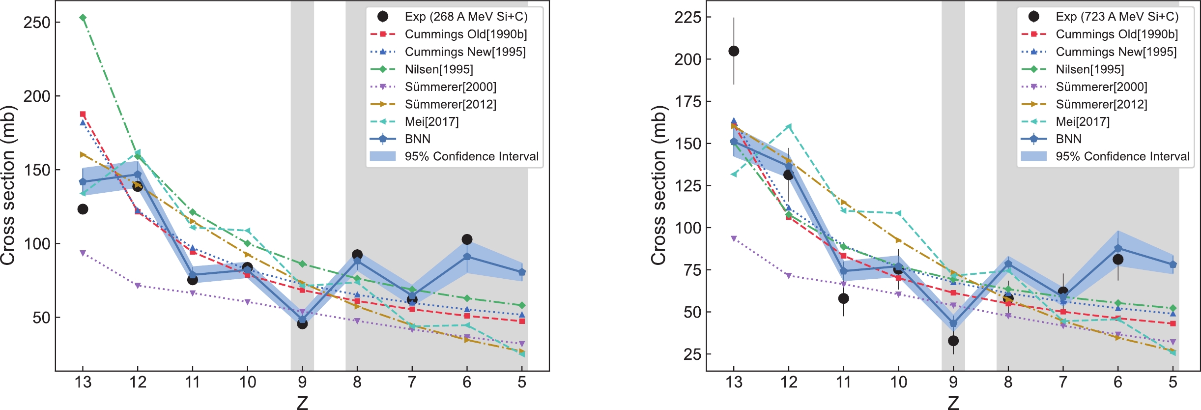
Figure 4. (color online) Predictions of the BNN method for the fragment production cross sections of
$ ^{28} {\rm{Si}}$ + C (268 A MeV) and$ ^{28} {\rm{Si}}$ + C (723 A MeV), along with comparisons with other theoretical models.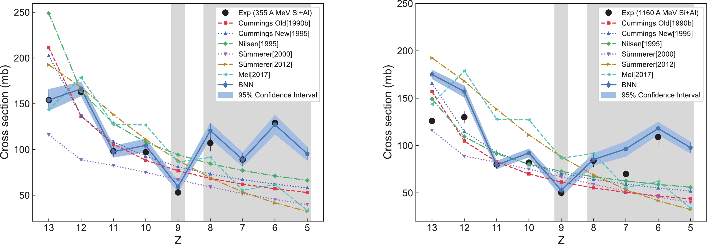
Figure 5. (color online) Predictions of the BNN method for the fragment production cross sections of
$ ^{28} {\rm{Si}}$ +Al (355 A MeV) and$ ^{28} {\rm{Si}}$ +Al (1160 A MeV), along with comparisons with other theoretical models.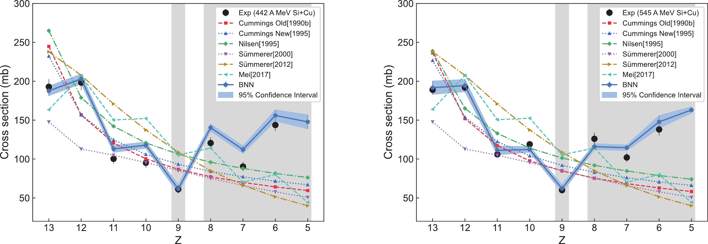
Figure 6. (color online) Predictions of the BNN method for the fragment production cross sections of
$ ^{28} {\rm{Si}}$ +Cu (442 A MeV) and$ ^{28} {\rm{Si}}$ +Cu (545 A MeV), along with comparisons with other theoretical models.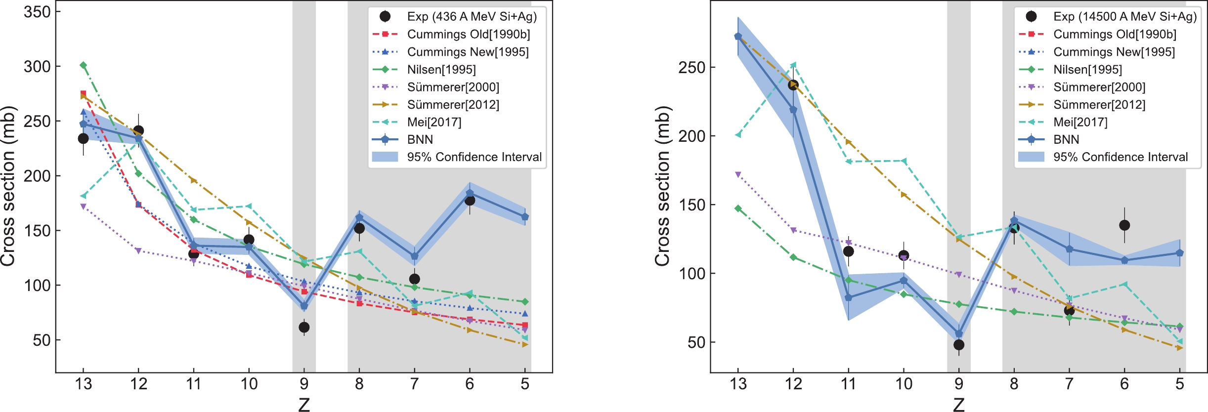
Figure 7. (color online) Predictions of the BNN method for the fragment production cross sections of
$ ^{28} {\rm{Si}}$ + Ag (436 A MeV) and$ ^{28} {\rm{Si}}$ + Ag (14500 A MeV), along with comparisons with other theoretical models.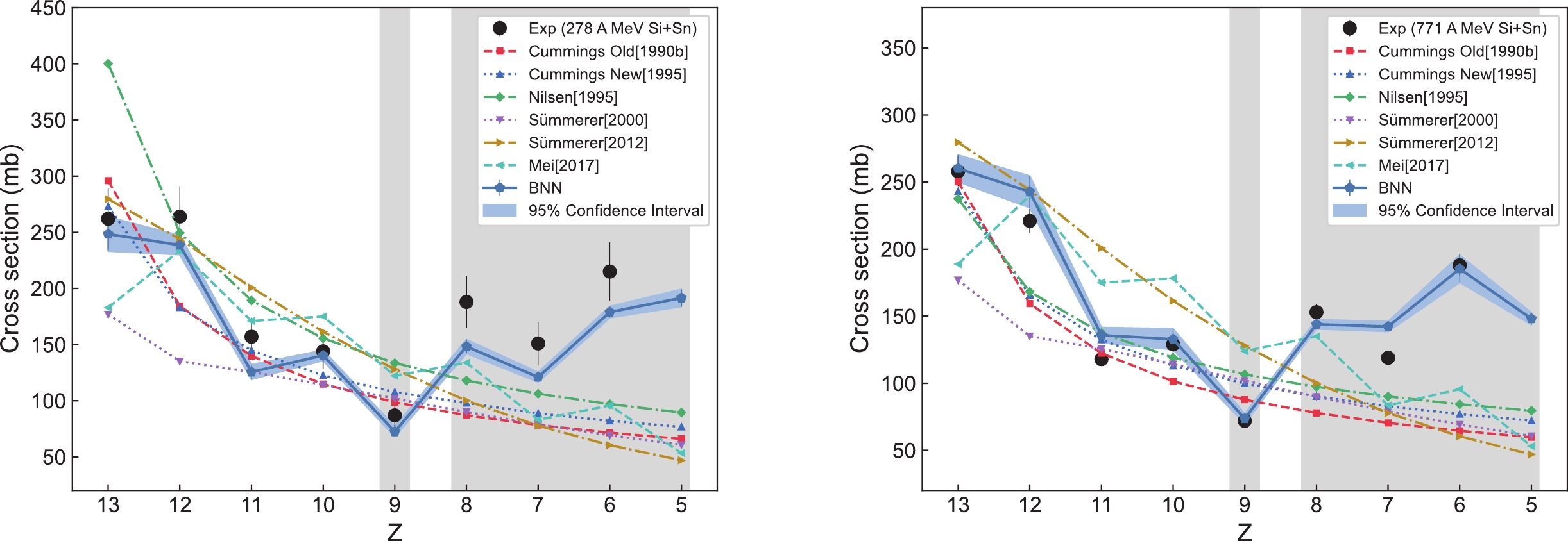
Figure 8. (color online) Predictions of the BNN method for the fragment production cross sections of
$ ^{28} {\rm{Si}}$ +Sn (278 A MeV) and$ ^{28} {\rm{Si}}$ +Sn (771 A MeV), along with comparisons with other theoretical models.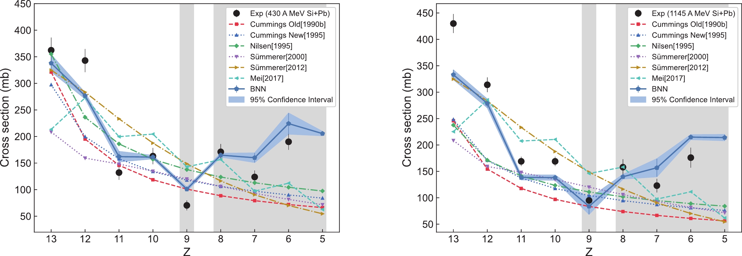
Figure 9. (color online) Predictions of the BNN method for the fragment production cross sections of
$ ^{28} {\rm{Si}}$ +Pb (430 A MeV) and$ ^{28} {\rm{Si}}$ +Pb (1145 A MeV), along with comparisons with other theoretical models.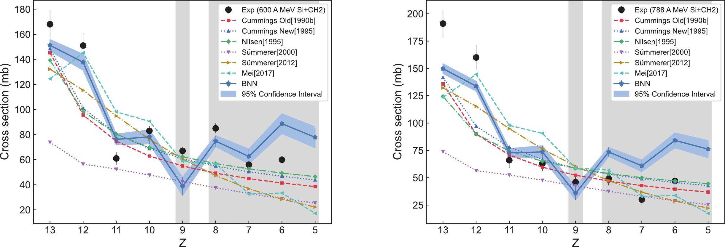
Figure 10. (color online) Predictions of the BNN method for the fragment production cross sections of
$ ^{28} {\rm{Si}}$ + CH$ _{2} $ (600 A MeV) and$ ^{28} {\rm{Si}}$ + CH$ _{2} $ (788 A MeV), along with comparisons with other theoretical models.For the odd-even staggering effect feature, which cannot be easily reproduced by traditional theoretical models, only the BNN method and the FRACS model show an obvious odd-even staggering effect. Notably, the BNN method reproduces the intensity of the odd-even staggering effect much closer to the experimental value, while the intensity of the FRACS model is weaker than the experimental value. Without adding additional input variables, we use BNN method to successfully reproduce the odd-even staggering feature and the data feature at
$Z = 9 $ presented in the experimental data. These successful prediction results fully demonstrate the reliability of our constructed neural network structure in capturing the inherent laws of complex data.Figure 11 shows the average ratio of predicted to experimental values for the different models with different fragment charges Z for all validation sets in Figs. 3−10. The figures show that only the BNN method exhibits an average ratio close to 1.0 between the predicted and experimental values for all the different fragment production charge cross sections.
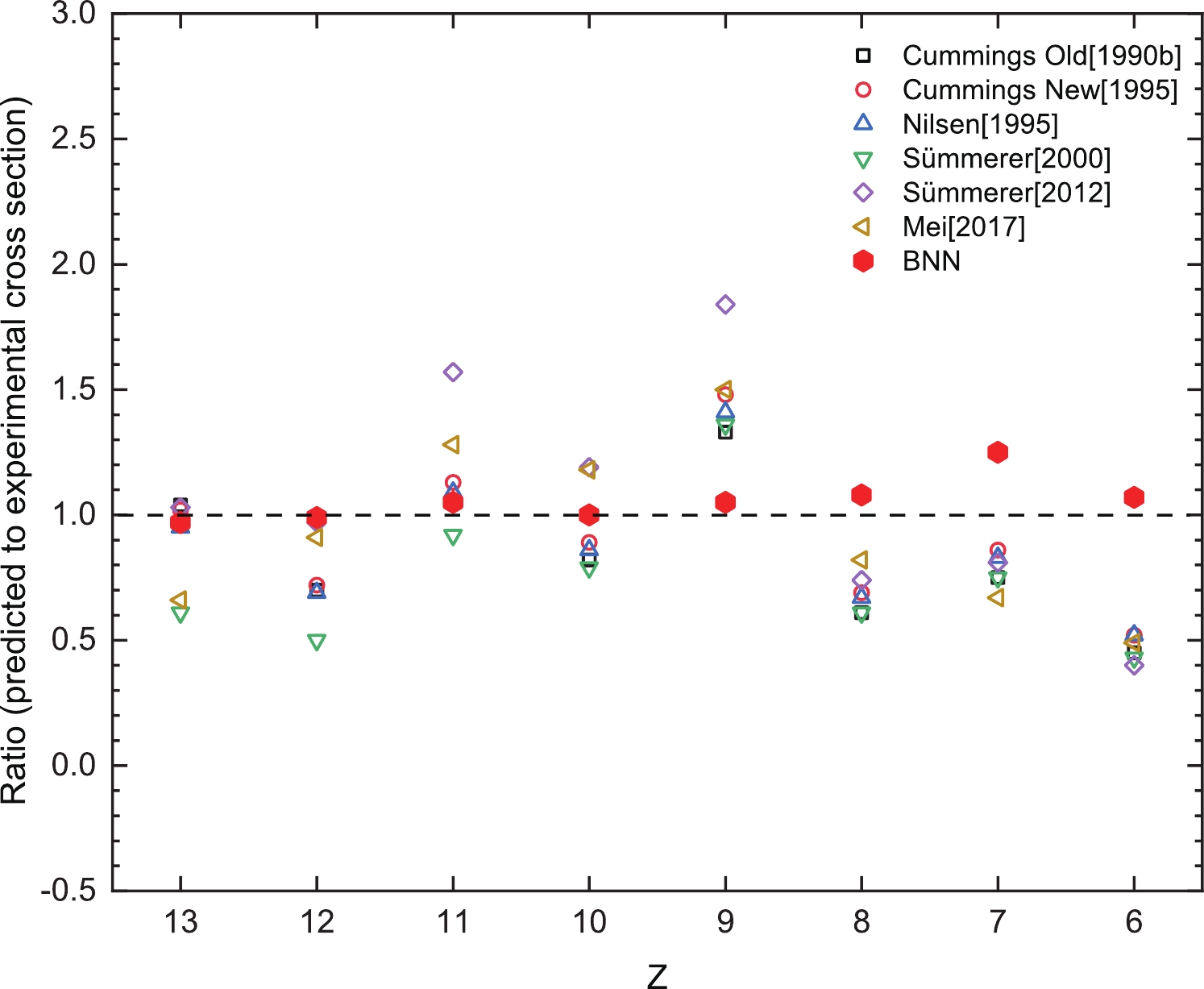
Figure 11. (color online) Average ratio of predicted to experimental values for different models with different fragment charges Z for all validation sets (V).
To further evaluate the accuracy of the BNN method, Fig. 12 shows a comparison of the RMSEs between the predicted and experimental values given by the BNN method and other theoretical models. After analyzing the data in the figure, we can clearly see that, compared with other theoretical models, the BNN method has a significantly lower RMSE between the predicted and experimental values. Table 3 lists the reduction rate of the RMSE for the BNN method compared to other theoretical models. From Table 3, we can see that, after learning through the BNN method, the average reduction rates of the RMSE value are 58%, 54%, 55%, 67%, 56%, and 58%, respectively, which are more than 50% compared with those of other theoretical models, and the degree of improvement is evident. These results show that the BNN method can significantly improve the prediction accuracy of the fragment production cross section, showing its good prediction ability.
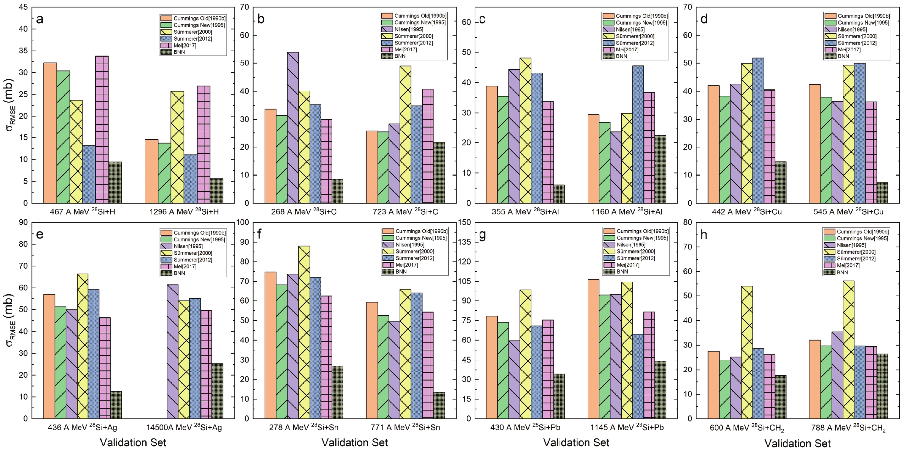
Figure 12. (color online) RMSEs between the predicted and experimental values given by the BNN method and other theoretical models.
Validation set (V) $\dfrac{\sigma_{\rm Cum.Old}-\sigma_{\rm BNN} }{\sigma_{\rm Cum.Old} }$ 

$\dfrac{\sigma_{\rm Cum.New}-\sigma_{\rm BNN} }{\sigma_{\rm Cum.New} }$ 

$\dfrac{\sigma_{\rm Nil.}-\sigma_{\rm BNN} }{\sigma_{\rm Nil.} }$ 

$\dfrac{\sigma_{\mathrm{S\ddot{u}m}.(2000)}-\sigma_{\rm BNN} }{\sigma_{\mathrm{S\ddot{u}m}.(2000)} }$ 

$\dfrac{\sigma_{\mathrm{S\ddot{u}m}.(2012)}-\sigma_{\rm BNN} }{\sigma_{\mathrm{S\ddot{u}m}.(2012)} }$ 

$\dfrac{\sigma_{\rm Mei}-\sigma_{\rm BNN} }{\sigma_{\rm Mei} }$ 

$^{28}{\rm{Si}}$ + H (467 A MeV)

0.71 0.69 — 0.60 0.28 0.72 $^{28}{\rm{Si}}$ + H (1296 A MeV)

0.61 0.59 — 0.78 0.49 0.79 $^{28}{\rm{Si}}$ + C (268 A MeV)

0.74 0.73 0.84 0.79 0.76 0.71 $^{28}{\rm{Si}}$ + C (723 A MeV)

0.16 0.15 0.24 0.56 0.38 0.47 $^{28}{\rm{Si}}$ + Al (355 A MeV)

0.84 0.83 0.86 0.87 0.86 0.82 $^{28}{\rm{Si}}$ + Al (1160 A MeV)

0.24 0.17 0.05 0.25 0.51 0.39 $^{28}{\rm{Si}}$ + Cu (442 A MeV)

0.65 0.61 0.65 0.70 0.72 0.64 $^{28}{\rm{Si}}$ + Cu (545 A MeV)

0.82 0.80 0.80 0.85 0.85 0.79 $^{28}{\rm{Si}}$ + Ag (436 A MeV)

0.78 0.75 0.75 0.81 0.79 0.73 $^{28}{\rm{Si}}$ + Ag (14500 A MeV)

— — 0.59 0.53 0.54 0.49 $^{28}{\rm{Si}}$ + Sn (278 A MeV)

0.64 0.61 0.63 0.69 0.63 0.57 $^{28}{\rm{Si}}$ + Sn (771 A MeV)

0.77 0.74 0.73 0.80 0.79 0.75 $^{28}{\rm{Si}}$ + Pb (430 A MeV)

0.57 0.54 0.43 0.65 0.52 0.55 $^{28}{\rm{Si}}$ + Pb (1145 A MeV)

0.59 0.53 0.53 0.58 0.32 0.46 $^{28}{\rm{Si}}$ + CH2 (600 A MeV)

0.36 0.27 0.30 0.67 0.39 0.33 $^{28}{\rm{Si}}$ + CH2 (788 A MeV)

0.18 0.11 0.25 0.53 0.11 0.10 Average value 0.58 0.54 0.55 0.67 0.56 0.58 Table 3. Reduction rate of the RMSE for the BNN method compared with other theoretical models in Fig. 12.
Finally, it should be noted that, when analyzing the experimental setup for group 8 as listed in Table 2, the data set involving
$ ^{28} {\rm{Si}}$ + Ag is not included in the training sets. However, from the results shown in Fig. 7 and Fig. 12(e), we can found that, compared with other theoretical models, the BNN method can show good prediction and reproduction performances for unseen reaction types, even in the absence of direct corresponding training data. This reflects the good generalization performance of the BNN method and further proves its reliability in dealing with complex and unknown data reaction types, thus providing a strong support for the future related research. -
In this study, the Bayesian neural network (BNN) method is used to accurately predict the fragment production cross section in the reaction of
$ ^{28} {\rm{Si}}$ with different targets at different energies. By analyzing the existing experimental data, we have successfully determined the optimal network structure of the BNN and made the corresponding prediction. The results demonstrate good prediction values and give the 95% confidence interval to quantify the uncertainty of the prediction. After comparing the prediction results of the BNN method with those of other theoretical models and experimental values, we find that, compared with those of the traditional theoretical model, the prediction results of the BNN method are more consistent with the experimental values. Notably, the prediction results of the BNN method show a clear odd-even staggering effect feature and data feature at Z = 9 without adding additional input parameters, which strongly demonstrates the excellent ability of the BNN method in capturing and reproducing complex data features. Further, we calculate the root-mean-square error (RMSE) between the predicted values of the BNN method and other theoretical models with the corresponding experimental values. The results show that the BNN method has the lowest RMSE value, which indicates that the BNN method significantly improves the prediction accuracy, demonstrating its strong ability to predict fragment production cross sections. These results provide a powerful tool for research in related fields and establish a solid foundation for subsequent theoretical and experimental exploration.
Predicting 28Si projectile fragmentation cross sections with Bayesian neural network method
- Received Date: 2024-06-27
- Available Online: 2024-12-15
Abstract: This study utilizes the Bayesian neural network (BNN) method in machine learning to learn and predict the cross-sectional data of 28Si projectile fragmentation for different targets at different energies and to quantify the uncertainty. The detailed modeling process of the BNN is presented, and its prediction results are compared with those of the Cummings, Nilsen, EPAX2, EPAX3, and FRACS models and experimental measurement values. The results reveal that, compared with other models, the BNN method achieves the smallest root-mean-square error (RMSE) and the highest agreement with the experimental values. Only the BNN method and FRACS model show a significant odd-even staggering effect; however, the results of the BNN method are closer to the experimental values. Furthermore, the BNN method is the only model capable of reproducing data features with low cross-section values at Z = 9, and the average ratio of the predicted to experimental values of the BNN is close to 1.0. These results indicate that the BNN method can accurately reproduce and predict the fragment production cross sections of 28Si projectile fragmentation and demonstrate its ability to capture key data characteristics.


 Abstract
 HTML
HTML Reference
 Related
 PDF
PDF




 DownLoad: