An empirical formula of nuclear β-decay half-lives with the transition-strength contribution

Nuclear β-decay is a process that involves the spontaneous conversion of one kind of nucleon to the other together with the emission of electron (or positron) and antineutrino (neutrino). It is one of the main decay modes of unstable nuclei [1, 2], which can provide the information on the spin and isospin dependence of the effective nuclear interaction and also on nuclear properties such as masses [3], shapes [4−6], and energy levels [7−9]. The origin of heavy elements in the universe has been one of the most extensively studied but least understood topics in nuclear astrophysics [10, 11]. In particular, about half of the elements heavier than iron are produced by the rapid-neutron capture process (r-process). Nuclear β-decay half-lives set the time scale of the r-process, which are important nuclear physics inputs for r-process simulations [12−15]. Therefore, the study of nuclear β-decay half-lives is of great value to nuclear physics and nuclear astrophysics [16−18]. However, most of the nuclei involved in the r-process are far away from the β stability line and cannot be accessed by the present experimental facilities. One has to rely on theoretical models for the prediction of the β-decay properties of those nuclei.

Theoretical models for the nuclear β-decay half-life studies include for example the gross theory [19−22], the shell model [13, 23−25], the quasiparticle random-phase approximation (QRPA) method [26−30], and the empirical formulas in various forms [31−34]. The gross theory is a macroscopic model based on a summation rule for β-decay strength function, and treats the transitions to all final nuclear levels in a statistical way. By introducing various microscopic effects, such as spin-parity property [35], spin-orbit splitting [36], the accuracy of gross theory can be remarkably improved and even higher than those from the microscopic models. However, some microscopic effects of gross theory are certainly missing due to the statistical way it adopts. On the other hand, the microscopic shell model configuration interaction approach can provide details of the β-strength function, but is often limited to study the nuclear β-decay half-lives of light nuclei or nuclei close to the magic number due to the computation limit in the large configuration spaces. The QRPA method can be applied to most nuclei in the nuclear chart except for a few very light nuclei [37−40], while the conventional QRPA calculations in the matrix form can be very time-consuming as well. The finite-amplitude method (FAM) was developed to solve QRPA equations [41, 42], which has been used to study the half-lives of medium-mass and heavy neutron-rich isotopes recently [43, 44]. However, the computation speed is still a very limiting factor if one intends to study all nuclei involved in the r-process, and its accuracy still needs to be improved in comparison to other nuclear β-decay models. Therefore, the construction of high-precision empirical formulas, which is much less time-consuming thanks to its simple form, can be the most promising and practical choice for systematically describing nuclear β-decay half-lives. We hope that a simple formula can describe the available experimental β-decay half-lives with high accuracy within around $ 10 $ parameters.

An empirical formula with higher prediction accuracy may be achieved by including more physical terms with their parameters determined by fitting to the experimental nuclear β-decay half-lives [32, 45]. Besides the proton number Z and the neutron number N, the calculation of the nuclear β-decay half-life with the empirical formula usually only requires the β-decay energy $ Q_\beta $, which can be calculated from the nuclear masses. Already at this point, the empirical formula of β-decay half-lives can be used to construct self-consistent nuclear β-decay half-life tables for various nuclear mass models, which is crucial for r-process studies, especially for the evaluation of the uncertainties of r-process abundances from the nuclear physical inputs. The empirical formula for the β-decay half-lives can be traced back to the Sargent law [46], which states that the nuclear β-decay half-lives are proportional to the fifth power of the maximum energy of the emitted electron. The Sargent law explains the $ Q_\beta $ value dependence of the β-decay half-life, but the prediction accuracy of this approximation is rather low due to the negligence of nuclear structure effects such as the shell effect, the pairing effect, and the isospin dependence. By further including these nuclear structure effects, the prediction accuracies of the empirical formulas have been improved remarkably [31, 32, 34].

In addition to the $ Q_\beta $, the β-decay transition strength also plays an important role in the half-life predictions. However, the transition-strength contribution is neglected in most existing empirical formulas. Recently, an empirical formula for the Gamow-Teller transition strength has been proposed [47] based on the Ikeda sum rule [48], the isospin symmetry, and the isospin limit condition. Based on that study of the transition strength, a new empirical formula for the nuclear β-decay half-lives is constructed in this work. The prediction accuracy and extrapolation ability of the new empirical formula are investigated by comparing its predictions with the experimental β-decay half-lives, the microscopic nuclear model predictions and those from other empirical formulas. The construction of the empirical formula is given in Sec. II. The corresponding results and discussion are given in Sec. III. The summary and perspective are presented in Sec. IV.

Based on the Fermi theory of β-decay [49], nuclear β-decay half-life $ T_{1/2} $ in the allowed Gamow-Teller approximation is

where $ D=2(\ln2)\pi^3\hbar^7/(m_e^5c^4g^2)=6163.4 $ s and $ g_A=1 $. $ B_{if_m} $ denotes the transition strength from the parent nucleus initial state i to the daughter nucleus final state $ f_m $, and $ f(Z,E_m) $ is the integrated phase volume, which can be calculated by

where $ m_e $, $ p_e $, $ E_e $, $ p_m $, $ E_m $, and $ F(Z,E_e) $ denote the mass, the momentum, the energy, the maximum momentum, the maximum energy, and the Fermi function of the emitted electron, respectively.

For nuclei with $ E_m \gg m_ec^2 $, if the Fermi integral function is further approximated by taking $ F(Z,E_e)\approx 1 $, one then gets

If only the transition from the ground state of the parent nucleus to the ground state of the daughter nucleus is considered, one can obtain from Eq. (1)

Neglecting the contribution of transition strength, setting the constants as free parameters $ a_1 $ and $ a_2 $, and taking $ E_{m}=Q_{\beta}+m_{e}c^{2} $, an empirical formula of the nuclear β-decay half-lives is obtained, named $ F_1 $,

To improve the performance of the empirical formula, the odd-even effect term $ \delta(Z, N)=(-1)^Z+(-1)^N $ and the shell effect correction term $ S(Z, N) $ are further introduced similar to Refs. [32] and [45]. One can get another empirical formula $ F_2 $,

with

The contribution of transition strength $ \sum_m B_{if_m} $ is neglected in the empirical formulas $ F_1 $ and $ F_2 $, while there are structure effects as well in $ \delta(Z, N) $ and $ S(Z, N) $ for the empirical formula $ F_2 $.

Recently, an empirical formula of the Gamow-Teller transition strength was proposed based on the Ikeda sum rule, the isospin symmetry, and the isospin limit condition in Ref. [47], i.e.

By further introducing the contribution of transition strength with Eq. (8), a new empirical formula $ F_3 $ is obtained, which is

In this work, we calculate $ Q_\beta $ values from the nuclear mass predictions of the Weizsäcker-Skyrme mass model (WS4) [50]. The experiment half-lives are taken from NUBASE2020 [2], while only the data for the nuclei with $ Z,\; N\geqslant8, $ $ Q_\beta>0 $, $ T_{1/2}<10^6\; {\rm{s}} $, and decaying $ 100\% $ by the $ \beta^- $ mode are retained. By fitting to the experimental half-lives, the parameters of the empirical formulas $ a_i\; (i=1, 2,...) $ can be determined, which are shown in Table 1.

Formula	$ a_1 $	$ a_2 $	$ a_3 $	$ a_4 $	$ a_5 $	$ a_6 $	$ a_7 $	$ a_8 $
$ F_1 $	12.267	5.712	—	—	—	—	—	—
$ F_2 $	12.254	6.035	0.540	4.989	6.331	3.492	1.188	—
$ F_3 $	14.608	6.164	0.545	3.985	5.882	3.610	1.608	0.498

Table 1.  The parameters of empirical formulas $ F_1 $, $ F_2 $, and $ F_3 $.

In order to evaluate the accuracy of empirical formulas for nuclear β-decay half-lives, we use the root-mean-square (rms) deviation of the logarithm of the half-life $ \sigma_{{\rm{rms}}}(\log_{10}T_{1/2}^{{\rm{Th}}}) $,

where $ T_{1/2}^{{\rm{Th}}} $ and $ T_{1/2}^{{\rm{Exp}}} $ are the theoretical and experimental half-life, respectively. n is the number of nuclei involved in the evaluation.

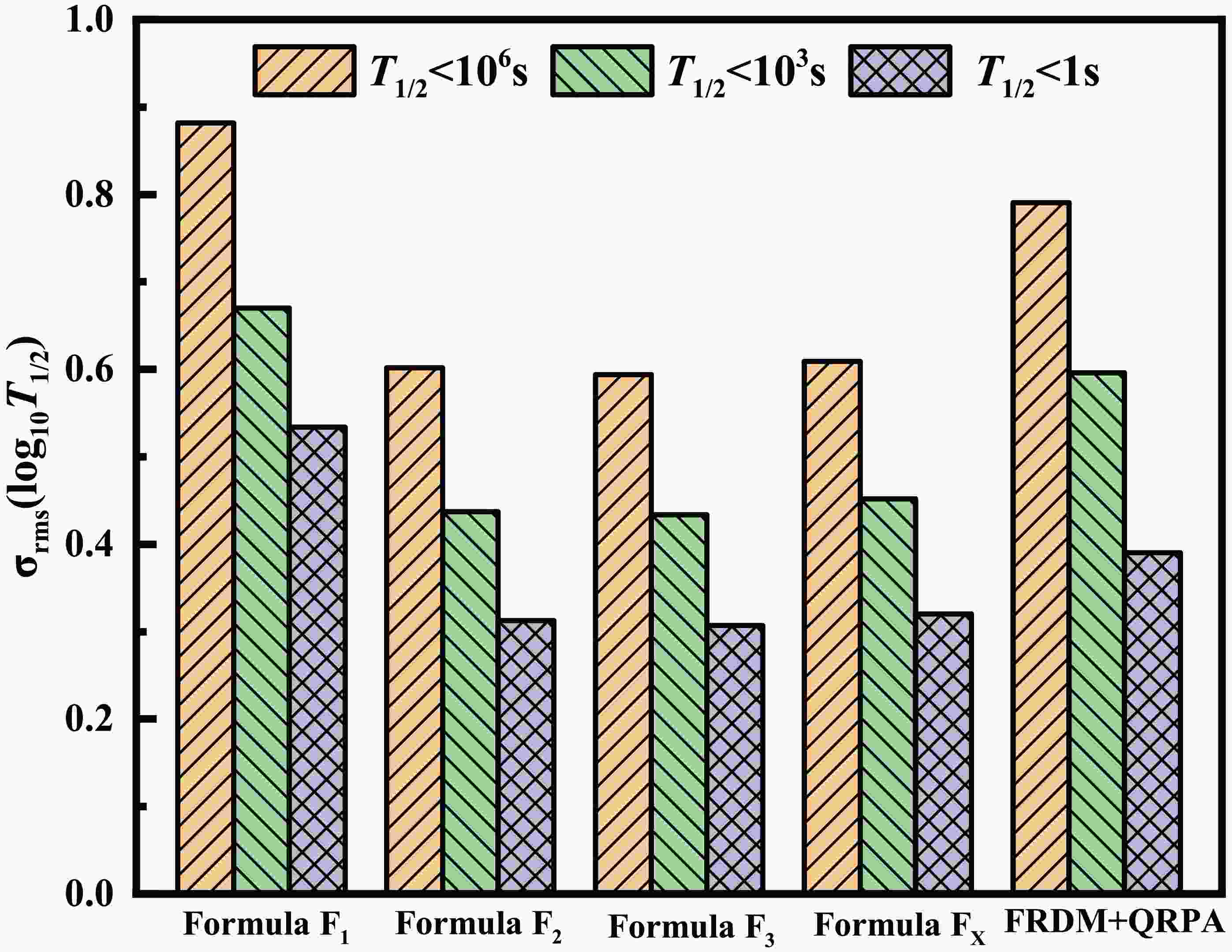
The prediction accuracies can be roughly evaluated by the rms deviations of the empirical formulas from the experimental half-lives, the rms deviations of the empirical formulas $ F_1 $, $ F_2 $, and $ F_3 $ are shown in Fig. 1, which are given for three data sets: $ T_{1/2}<10^{6}\; {\rm{s}} $, $ T_{1/2}<10^{3}\; {\rm{s}} $, and $ T_{1/2}<1\; {\rm{s}} $. The results of the empirical formula $ F_{{\rm{X}}} $ from Ref. [45] and the QRPA based on the finite-range droplet model (FRDM+QRPA) [37] are also given. For a fair comparison, the parameters of $ F_{{\rm{X}}} $ are also refitted using the same data in this work. As shown in Fig. 1, the rms deviations of the theoretical half-lives with respect to the experimental data become smaller and smaller from the data set $ T_{1/2}<10^{6}\; {\rm{s}} $ to the data set $ T_{1/2}<10^{3}\; {\rm{s}} $ to the data set $ T_{1/2}<1\; {\rm{s}} $, which indicates that the β-decay models describe the shorter half-lives better. Compared with $ F_1 $, the rms deviations of $ F_2 $ are effectively reduced by introducing the odd-even effect and the shell correction effect, the accuracies of $ F_2 $ are improved by $ 31.7\% $, $ 34.8\% $, and $ 41.4\% $ for $ T_{1/2}<10^{6}\; {\rm{s}} $, $ T_{1/2}<10^{3}\; {\rm{s}} $, and $ T_{1/2}<1\; {\rm{s}} $, respectively. By including the transition-strength contribution on $ F_2 $, the accuracy of $ F_3 $ further improved by about $ 1\% $. For $ T_{1/2}<1\; {\rm{s}} $, the empirical formula $ F_3 $ provides the best description of the experimental half-lives, reproducing the experimental half-lives even within $ 10^{0.307} \approx 2 $ times. The accuracies of $ F_3 $ and $ F_{{\rm{X}}} $ are similar for the three data sets, both of which are better than those of the microscopic FRDM+QRPA model. It should be pointed out that $ F_{{\rm{X}}} $ includes other additional terms related to $ \alpha^2 Z^2 $, $ \alpha Z $, and $ (N-Z)/A $. The small differences between the rms deviations of $ F_2 $, $ F_{{\rm{X}}} $, and $ F_3 $ show that the transition-strength contribution can be effectively taken into account by refitting the parameters of other terms, however, the differences between the predictions of $ F_2 $, $ F_{{\rm{X}}} $, and $ F_3 $ may become larger and larger when extrapolated to the unknown region, which will be investigated below.

Figure 1.  (Color online) The rms deviations $ \sigma_{{\rm{rms}}}(\log_{10}T_{1/2}^{{\rm{Th}}}) $ of the empirical formulas $ F_1 $, $ F_2 $ and $ F_3 $ with respect to experimental data from NUBASE2020 [2] for three data sets $ T_{1/2}<10^{6}\; {\rm{s}} $, $ T_{1/2}<10^{3}\; {\rm{s}} $, and $ T_{1/2}<1\; {\rm{s}} $. The predictions of the empirical formula $ F_{{\rm{X}}} $ and the microscopic model FRDM+QRPA are shown for comparison.

To investigate the role of the transition strength in the calculation of β-decay half-lives, we design an empirical formula named $ F_{3}^{\prime} $ by removing the transition-strength term, i.e. taking $ a_8 = 0 $ in the empirical formula $ F_3 $. The comparison between the half-life predictions of $ F_3 $ and $ F_{3}^{\prime} $ is shown in Fig. 2 by taking Ca, Ni, Sn, and Pb isotopes as examples. It can be seen that the transition strength reduces the predictions of nuclear β-decay half-lives by about an order of magnitude, which shows the transition strength plays an important role in predicting nuclear β-decay half-lives. From Eq. (8), the transition strength $ \sum B_{ {\rm{GT-}}} \rightarrow 3(N-Z) $ when $ N \gg Z $, which is in agreement with the Ikeda sum rule since the Gamow-Teller transition from $ (Z, N) $ to $ (Z-1, N+1) $ is forbidden when $ N \gg Z $. Therefore, the transition-strength contribution gradually increases toward the neutron-rich regions with larger $ (N-Z) $, which can be observed in the Ca, Ni, Sn, and Pb isotopes from Fig. 2. The heavy nuclei generally have larger $ (N-Z) $ than the light nuclei, so the transition-strength contribution is generally larger in the Pb isotope than in the Ca isotope when extrapolated to the unstable neutron-rich region. This indicates that the transition-strength contribution is more important for the neutron-rich nuclei in the heavy nuclear region.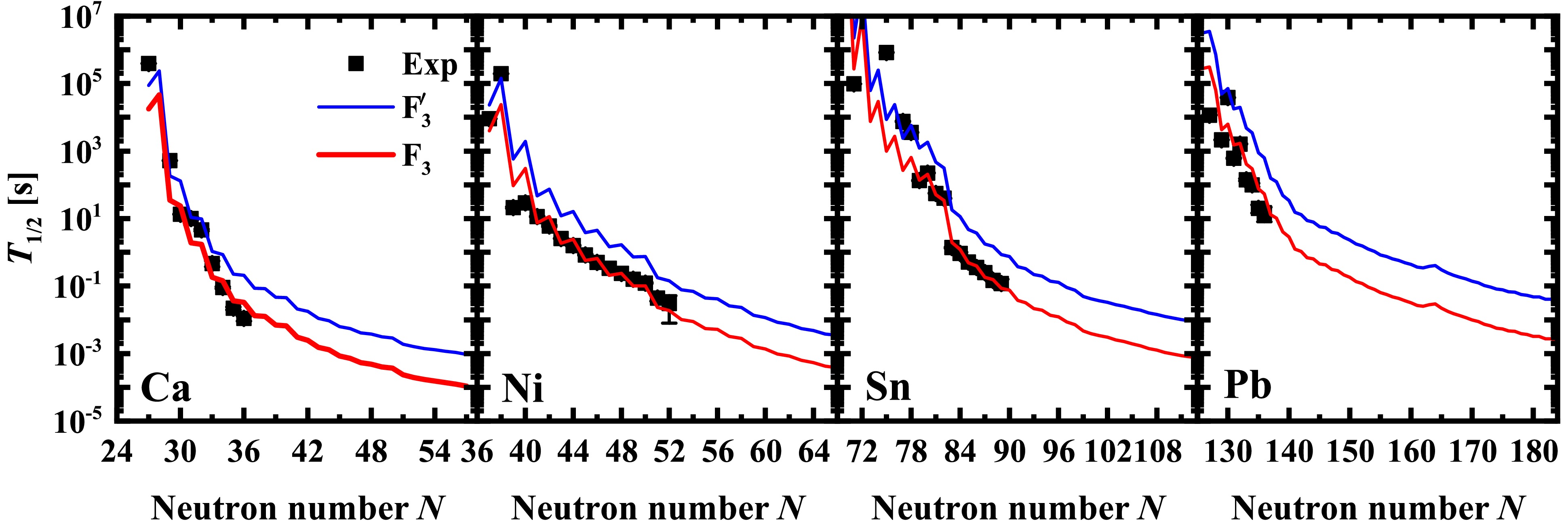

Figure 2.  (Color online) Nuclear β-decay half-lives of Ca, Ni, Sn, and Pb isotopes predicted by $ F_{3}^{\prime} $ and $ F_3 $. The experimental data from NUBASE2020 are denoted by filled squares.

To compare the nuclear β-decay half-lives predicted by various empirical formulas, the predictions of $ F_1 $, $ F_2 $, $ F_3 $, and $ F_{{\rm{X}}} $ are shown in Fig. 3 by taking Ca, Ni, Sn, and Pb isotopes as examples. The predictions of $ F_1 $ have an excessive odd-even staggering in the known region, which is effectively reduced by $ F_2 $, $ F_3 $, and $ F_{{\rm{X}}} $ through introducing a physical quantity δ. As discussed above, the transition-strength contribution can be effectively taken into account by refitting the parameters of the $ F_2 $ and $ F_{{\rm{X}}} $, so the $ F_2 $, $ F_{{\rm{X}}} $, and $ F_3 $ generally give very similar half-life predictions in the known region. However, the deviations between them become larger and larger when extrapolated to the unknown region. Specifically, there are large deviations between the $ F_{{\rm{X}}} $ and $ F_3 $ predictions in the light nuclear region for Ca and Ni isotopes, and between the $ F_2 $ and $ F_3 $ predictions in the medium and heavy nuclear region for Sn and Pb isotopes.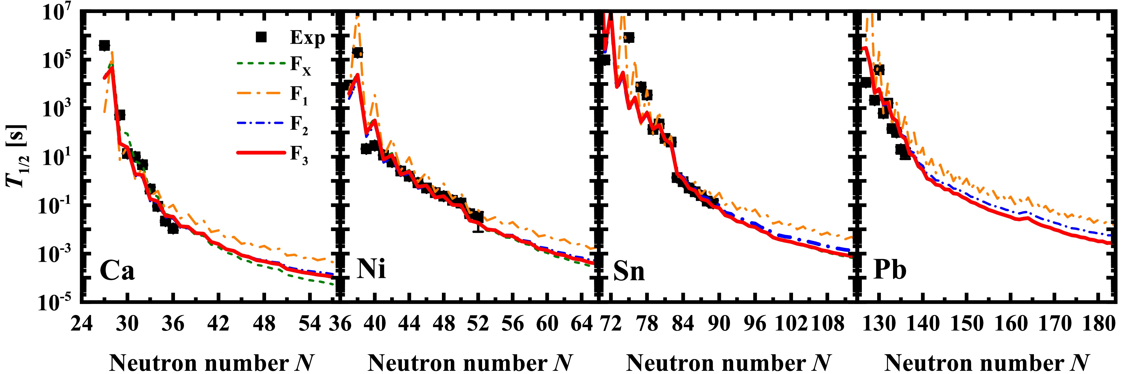

Figure 3.  (Color online) Nuclear β-decay half-lives of Ca, Ni, Sn, and Pb isotopes predicted by $ F_{{\rm{X}}} $, $ F_1 $, $ F_2 $, and $ F_3 $ which are shown by short dashed, dash-dotted, short-dotted, and solid lines, respectively.

To show the transition-strength contribution to the half-life predictions globally, Figure 4(a) shows the logarithmic differences between $ F_3 $ and $ F_{3}^{\prime} $ half-life predictions, it is found that the transition-strength contribution to the nuclear β-decay half-lives gradually increases toward neutron-rich or heavy nuclear regions, which is in agreement with the conclusion presented in Fig. 2. As mentioned above, the transition-strength contribution can be effectively taken into account by refitting the parameters of $ F_2 $, and the logarithmic differences between $ F_3 $ and $ F_2 $ half-life predictions are shown in Fig. 4(b). Clearly, the difference between $ F_3 $ and $ F_2 $ is less than $ 0.3 $ orders of magnitude for many nuclei, however, there is still larger systematic overestimation of β-decay half-lives for neutron-rich nuclei in heavy nuclear region. In addition, a large systematic underestimation of β-decay half-lives is also found for the nuclei near the β stability line in light nuclear region. Therefore, the inclusion of the transition-strength contribution in the empirical formula is crucial for the global description of nuclear β-decay half-lives, especially for the light or heavy neutron-rich nuclei. It should be pointed out that, on the one hand, $ F_2 $ and $ F_3 $ give better predictions for different nuclei, and on the other hand, there are only a few known nuclei with large deviations between $ F_2 $ and $ F_3 $ predictions, which are mainly concentrated in the light nuclear region near the stability line as shown in Fig. 4, while the rms deviation is an average result for all the known nuclei. Therefore, there are similar rms deviations for $ F_2 $ and $ F_3 $ in Fig. 1.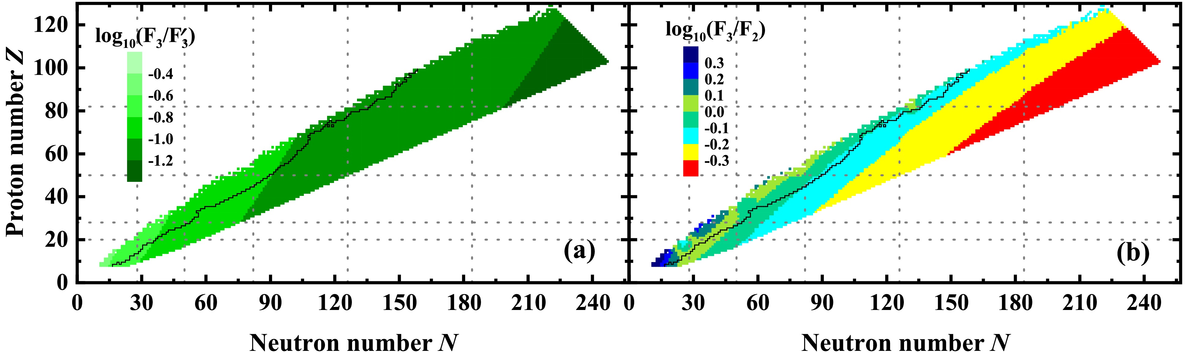

Figure 4.  (Color online) The logarithmic differences between the half-life predictions of $ F_3 $ and $ F_{3}^{\prime} $ (a), $ F_3 $ and $ F_2 $ (b). The solid line represent the boundary of nuclei with known half-lives in NUBASE2020 [2].

The logarithmic difference between the experimental half-lives and the predictions of $ F_3 $ is shown in Fig. 5. Clearly, there are large deviations between the $ F_3 $ predictions and the experimental data for the nuclei near the β stability line, whose half-life description is also a great challenge for other empirical formulas and microscopic models. For nuclei with shorter half-lives far away from the β stability line, the empirical formula $ F_3 $ can generally reproduce the experimental half-lives within $ 0.4 $ orders of magnitude.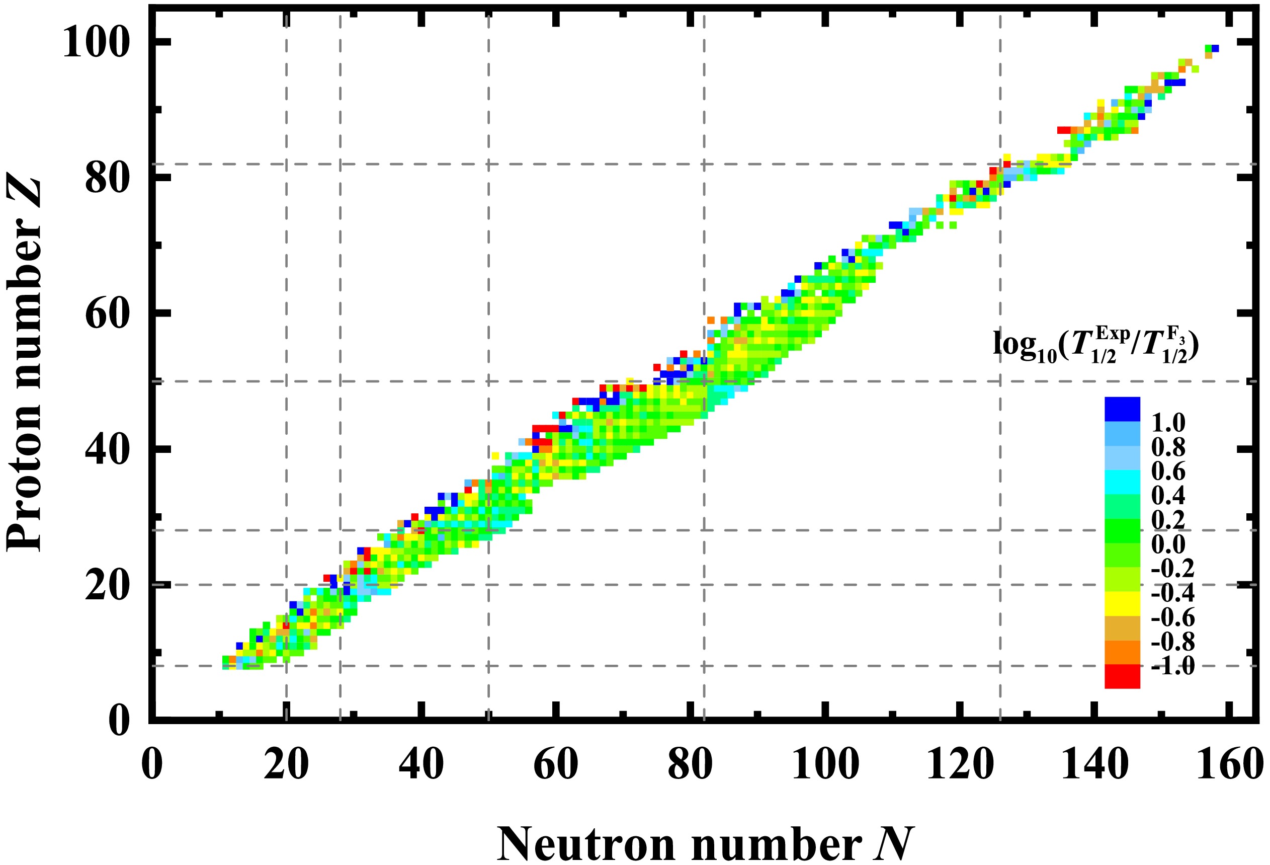

Figure 5.  (Color online) Logarithmic differences between the experimental β-decay half-lives and $ F_3 $ predictions. The dashed lines denote the traditional magic numbers.

Taking Ca, Ni, Sn, and Pb isotopes as examples, Figure 6 shows the comparison between the results of $ F_3 $ and other microscopic models, including the FRDM+QRPA [37], the QRPA based on the Relativistic Hartree-Bogoliubov (RHB+QRPA) [38], the FAM based on the Hartree-Fock-Bogoliubov model with Skyrme force (SHFB+FAM) [44], and the SHFB+QRPA [51] models. It can be seen that the predictions of $ F_3 $ are much better than other microscopic models. Quantitatively, for Ca, Ni, Sn, and Pb isotopes, the rms deviations of the FRDM+QRPA, RHB+QRPA, SHFB+FAM, and SHFB+QRPA half-life predictions from the experimental data are $ 0.833 $, $ 1.887 $, $ 0.940 $, and $ 0.923 $, respectively, while it is only $ 0.679 $ for the $ F_3 $. When extrapolated to the unknown region, the $ F_3 $ predictions are systematically shorter than those from other microscopic models for the light nuclei near the neutron-drip line, such as the Ca and Ni isotopes; while the $ F_3 $ predictions are between those of the other microscopic models for the heavy nuclei, such as the Pb isotopes.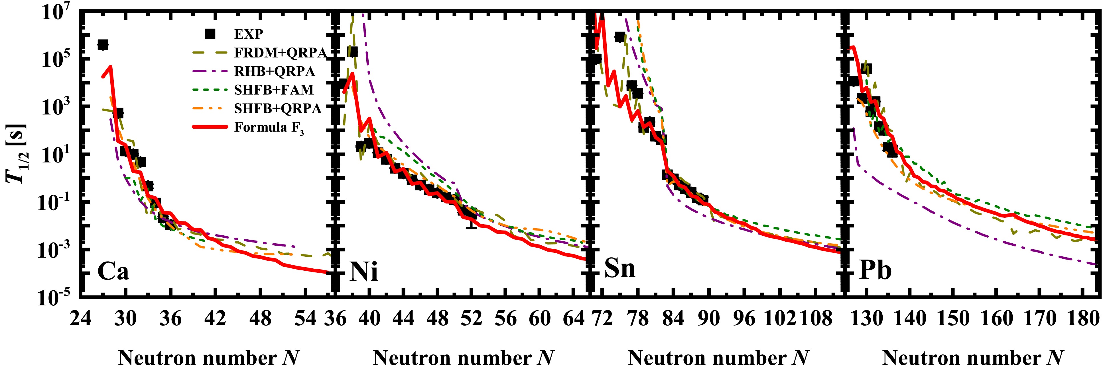

Figure 6.  (Color online) Nuclear β-decay half-lives of Ca, Ni, Sn, and Pb isotopes predicted by $ F_3 $. For comparison, the theoretical results of FRDM+QRPA, RHB+QRPA, SHFB+FAM, and SHFB+QRPA are shown by the dashed, dash-dotted, short dashed, dash-dot-dotted, respectively.

The new measurements of nuclear β-decay half-lives from Ref. [52], which are not involved in the fitting of the empirical formula, are further used to check the extrapolation ability of the empirical formula $ F_3 $, which are presented in Fig. 7. The experimental data from NUBASE2020 and the results from the FRDM+QRPA model are also shown for comparison. The empirical formula $ F_3 $ reproduces the newly measured half-lives of the Pm isotopes better than the FRDM+QRPA model, which systematically underestimates these half-life data. For the Sm, Eu, and Gd isotopes, both the empirical formula $ F_3 $ and the FRDM+QRPA reproduce the newly measured half-lives well. Quantitatively, the rms deviation of the FRDM+QRPA predictions from the newly measured half-lives for the four isotopes is $ 0.294 $, while it is only $ 0.209 $ for the empirical formula $ F_3 $. Therefore, the empirical formula $ F_3 $ provides a reliable prediction of the nuclear β-decay half-lives, at least for nuclei not far from the known region.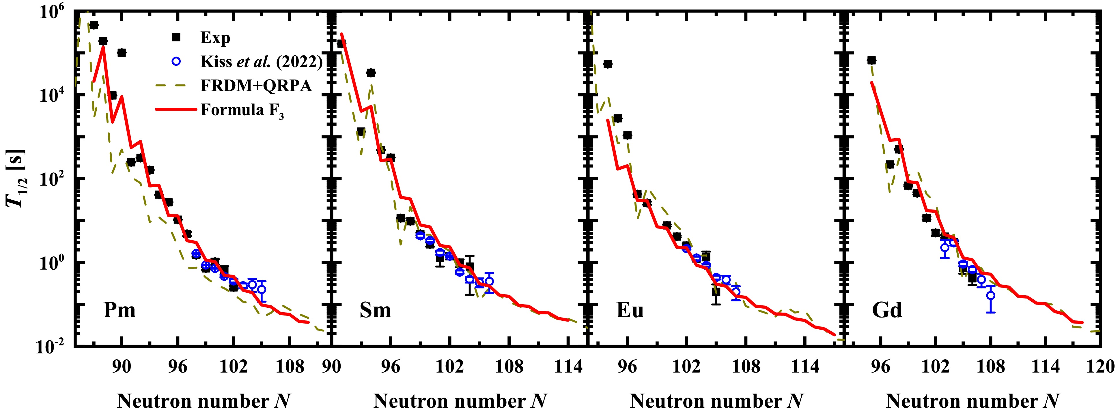

Figure 7.  (Color online) Nuclear β-decay half-lives for Pm, Sm, Eu, and Gd isotopes. The experimental half-lives from NUBASE2020 [2] and the newly measured data [52] are denoted by the filled squares and open circles. The FRDM+QRPA half-life predictions are shown by the dashed lines for comparison.

In summary, an empirical formula of nuclear β-decay half-lives is proposed by including the transition-strength contribution. The new empirical formula can describe the β-decay half-lives better than other empirical formulas and microscopic models. For the nuclei with half-lives less than $ 1 $ second, the rms deviation of the predictions of the new empirical formula from the experimental half-lives is only $ 0.307 $, which means that it can reproduce the experimental data within about $ 2 $ times. It is found that the inclusion of the transition-strength contribution can reduce nuclear β-decay half-lives by about an order of magnitude. The effect can increase further toward the neutron-rich or heavy nuclear regions with large $ (N-Z) $. The transition-strength contribution can also be taken into account effectively by refitting the parameters of other empirical formulas without transition-strength term. However, there are still remarkable deviations from the predictions of the new empirical formula for the neutron-rich nuclei in the light or heavy nuclear regions, indicating that the transition strength is crucial for the global description of nuclear β-decay half-lives. Furthermore, we analyze the extrapolation ability of the empirical formula by comparing it to the newly measured nuclear β-decay half-lives not involved in the fitting procedure. It is found that the new empirical formula describes the nuclear β-decay half-lives well, at least for nuclei not far from the known region. In the future, it is possible to provide a high-precision nuclear β-decay half-life table for various mass models based on this empirical formula, which can be used in the r-process calculations, and to further study its impact on the r-process simulations.

We are grateful to Professor Chong Qi for the valuable suggestions.