Evolution of the universe prior to inflation in loop quantum cosmology

I. INTRODUCTION

• I. INTRODUCTION
• II. EVOLUTION OF PRE-INFLATIONARY UNIVERSE
•      A Model 1: $V(\phi) \propto \phi^{4}$
•      B Model 2: $V(\phi) \propto (1+\phi)^2$
• III. PHASE SPACE ANALYSIS
• IV. CONCLUSIONS
• ACKNOWLEDGMENT
• APPENDIX A: PHYSICAL QUANTITIES

The theory of inflation was suggested in 1980. Since then, it has been notably successful in solving many relevant problems of the Big Bang cosmology, such as the horizon and flatness problems. Cosmic inflation explains the origin of inhomogeneities and the structure formation of the universe [1, 2]. However, knowledge on its past is incomplete owing to the initial singularity, known as the Big Bang singularity, where all quantities become infinite. Over the past two decades, loop quantum cosmology (LQC) has been employed to resolve the Big Bang singularity in cosmological models. Within the framework of LQC, quantum geometric effects play a crucial role, replacing the initial singularity with a non-singular quantum bounce [3−5]. LQC is a successful application of loop quantum gravity (LQG) [6,7]. Based on Ashtekar's variables and the Hamiltonian formalism, LQG is a canonical quantization of Einstein's theory of gravity [8]. LQC is built by applying LQG methods on cosmological models in the context of the supermini-space methodology [3]. LQC addresses the Big-Bang singularity through a generic approach [9]. The use of LQC in inflationary cosmology is motivated by its ability to resolve the initial singularity and provide a more comprehensive understanding of the universe's origins. Let us explore some of these motivations in detail. The first key motivation is the resolution of the singularity. LQC offers a framework that replaces the Big Bang singularity with a quantum bounce. In this scenario, the universe undergoes a phase of contraction to an extent before expanding again. This bounce offers a natural mechanism for transitioning from a pre-inflationary phase to an inflationary phase, which is essential for inflationary models. The second motivation lies in the incorporation of quantum gravitational effects. LQC accounts for these effects at high densities, significantly influencing the early universe's dynamics. This can address longstanding issues such as the flatness and horizon problems. Furthermore, LQC provides insights into the behavior of scalar fields during inflation and how quantum fluctuations may manifest in cosmic microwave background radiation. Concerning the implications of LQC for inflationary cosmology, the dynamics of inflation can be affected by the bounce. This can, in turn, modify the predictions about the scalar power spectrum and tensor-to-scalar ratio. Additionally, the bounce introduces novel quantum effects that modify the spectrum of perturbations. By resolving the initial singularity, LQC offers a new perspective on the universe's initial conditions. Rather than emerging from a singular state, the universe transitions from a pre-bounce state, which can influence the scalar field configurations and the duration of inflation. Recently, an extensive study on the modified Loop Quantum Cosmology (mLQC) was reported [10−15]. Two fundamental gradients were adopted to derive mLQC: the first one is the supermini-space assumption; the second one is the classical relation between the Euclidean and Lorentzian terms. However, none of them exhibit the essence of LQG, in which the quantizations of the Euclidean and Lorentzian terms usually follow different processes [9], and the operations of symmetry reduction and quantization are not communicated. In Ref. [16], the effective Hamiltonian was obtained by closely following the processes of LQG. Later, a systematical derivation of the effective Hamiltonian was reported in Refs. [17−19]. In this context, various scalar field models were systematically studied in the post-bounce phase [20−22].

In this study, we investigated the evolution of the universe with different potentials in the context of LQC and numerically obtained initial conditions of the inflaton field at the bounce. Furthermore, we thoroughly studied the initial conditions of the field to check the slow-roll inflation. All inflationary models, in the case of the classical theory of General Relativity (GR), are affected by the Big Bang singularity, which is inevitable [23, 24]. Hence, it is difficult to know when and how to set the initial values of the field. To be consistent with observations, the number of e-folds should be at least 60 during the slow-roll inflation for each value of the inflaton field; if this is not the case, such a value of the field would be discarded. The number of e-folds, in some cases, exceeds 70 [25]. In this study, we used only background cosmology to demonstrate the numerical evolution of the universe. In the case of kinetic energy dominated (KED) initial values of the inflaton field, the universe is divided into three distinct regimes: bouncing, transition, and slow-roll inflation. Conversely, the bouncing and transition regimes are absent in potential energy dominated (PED) initial conditions of the inflaton field. To review the dynamical behavior of pre-inflation and inflation, readers may consult Refs. [26−34]. The choice of power law potentials (see models 1 and 2) in the context of LQC is often motivated by their simplicity and mathematical tractability, rather than their direct observational agreement with current cosmological data. Power law potentials are among the simplest types of potentials used to study inflationary dynamics in cosmology. Their straightforward mathematical forms lead to relatively simple solutions for field dynamics in both classical and quantum gravity contexts. In LQC, these potentials serve as a good starting point for understanding how quantum gravity influences inflation, even if they do not necessarily align with current observations. While present observations (e.g., Planck data) favor smaller field potentials such as the Starobinsky potential, the study of models 1 and 2 remains important for theoretical exploration. The fact that these potentials may be ruled out by observations does not invalidate their role in LQC studies. Instead, they offer valuable insights into the structure of inflationary models, even if they do not perfectly align with observational data. In this sense, studying these potentials acts as a stepping stone for understanding a broader range of potential behaviors within LQC.

This paper is organized as follows. In Sec. II, the evolution equations of LQC with a spatially flat Friedmann–Lemaître–Robertson–Walker (FLRW) universe is discussed. In sub-sections II.A and II.B, we examine the numerical evolution of the models with $V(\phi) \propto \phi^{4}$ and $V(\phi) \propto (1+\phi)^2$ and check whether the desired slow-roll inflation with at least 60 e-folds exists. Sec. III is devoted to phase space analysis. The results are summarized in Sec. IV.

II. EVOLUTION OF PRE-INFLATIONARY UNIVERSE

• I. INTRODUCTION
• II. EVOLUTION OF PRE-INFLATIONARY UNIVERSE
•      A Model 1: $V(\phi) \propto \phi^{4}$
•      B Model 2: $V(\phi) \propto (1+\phi)^2$
• III. PHASE SPACE ANALYSIS
• IV. CONCLUSIONS
• ACKNOWLEDGMENT
• APPENDIX A: PHYSICAL QUANTITIES

In this section, we review the dynamics of pre-inflation in a homogeneous and isotropic FLRW background with a spatially flat metric described by

where t is the cosmic time and $a(t)$ represents the expansion factor of the universe. The modified Friedmann equation with a spatially flat FLRW universe in the framework of LQC is given by [7]

where $m_{pl}^2 = 1/G$ denotes the Planck mass; ρ and $\rho_c$ represent the energy density of the scalar field and the critical energy density, respectively; $\rho_c$ is approximated as $\rho_c \simeq 0.41 m_{pl}^4$ [35, 36]; $H = \dot{a}/a$ is the Hubble parameter; and dot $(.)$ denotes differentiation with respect to cosmic time. In this paper, we consider single field inflation, for which the Klein-Gordon equation is expressed as

The equation of state (EOS) $w(\phi)$ for the scalar field is defined as

In LQC, the Big Bang singularity is resolved and replaced by a non-singular quantum bounce [3−5, 16]. At $\rho = \rho_c$ , the quantum bounce occurs where the Hubble parameter becomes zero ( $H = 0$ ) (see Eq. (2)). The numerical evolution of the background for various potentials has been investigated in the literature [26, 28, 30, 32, 34]. An important result is that the desired slow-roll inflationary regime is achieved. In the present study, we chose generic potentials of the form $V(\phi) \propto \phi^{4}$ and $V(\phi) \propto (1+\phi)^2$ and investigated the dynamics of the pre-inflationary universe. Before addressing these potentials, let us discuss the background described by Eqs. (2) and (3) for a general form of the potential $V(\phi)$ . Eqs. (2) and (3) can be solved by imposing initial conditions on $a(t)$ , $\phi(t)$ , and $\dot{\phi}(t)$ at the bounce $(t = t_B)$ ; therefore, at the bounce, we have

which yields

For the sake of simplicity, hereafter, we express $\phi(t_B ), \dot{\phi}(t_B)$ and $a(t_B)$ as $\phi_B, \dot{\phi}_B$ and $a_B$ , respectively. The $\pm$ sign in Eq. (6) means that $\dot{\phi}_B>0$ (positive inflaton velocity; PIV) or $\dot{\phi}_B<0$ (negative inflaton velocity; NIV) at the bounce. Next, we define several quantities that are used in the paper.

The analytical expression of the scale factor $a(t)$ in the bouncing regime is given by [37, 38]

where $a_B = 1$ , $\delta = {24 \pi \rho_c}/{m_{Pl}^{4}}$ is a dimensionless parameter, and $t_{Pl}$ denotes the Planck time. The slow-roll parameter $\epsilon_H$ and number of $e-$ folds $N_{inf}$ are defined as

where $a_i$ and $a_{\rm end}$ represent the scale factor at the onset and end of the inflation, respectively, i.e., $\ddot{a}(t_i)\gtrsim 0$ and $w_{\phi}({\rm{end}}) = -1/3$ . In the following sub-section, we investigate the initial conditions of pre-inflation using the models under consideration for $\dot{\phi}_B>0$ at the quantum bounce. A similar analysis can be conducted for $\dot{\phi}_B<0$ , but we restrict ourselves to $\dot{\phi}_B>0$ only.

A Model 1: $V(\phi) \propto \phi^{4}$

• I. INTRODUCTION
• II. EVOLUTION OF PRE-INFLATIONARY UNIVERSE
•      A Model 1: $V(\phi) \propto \phi^{4}$
•      B Model 2: $V(\phi) \propto (1+\phi)^2$
• III. PHASE SPACE ANALYSIS
• IV. CONCLUSIONS
• ACKNOWLEDGMENT
• APPENDIX A: PHYSICAL QUANTITIES

Let us study the bounce and slow-roll inflation with quartic potential:

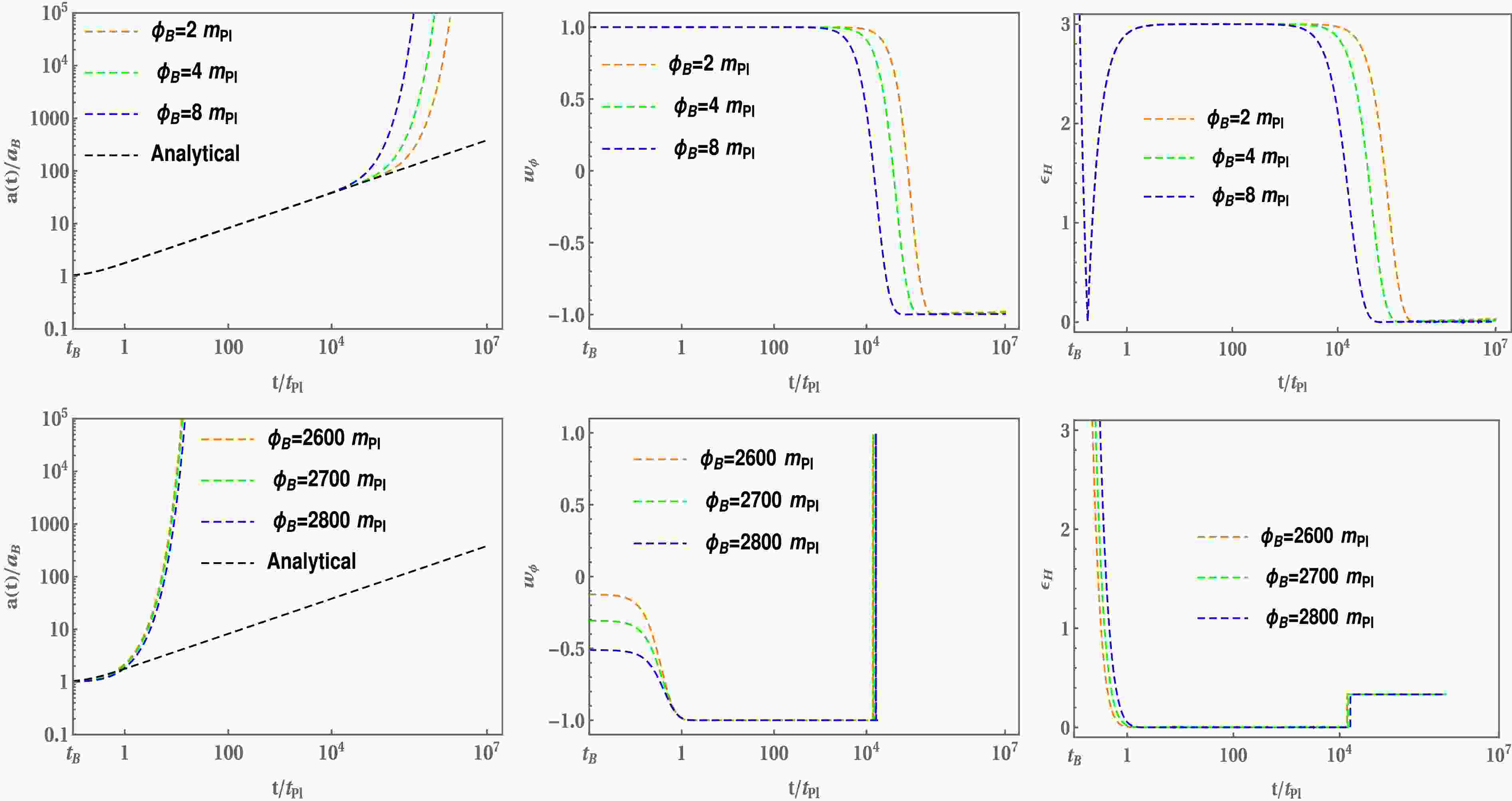
We set $V_0 = 2.01559 \times 10^{-14}m_{Pl}^4$ (see Appendix). Next, we numerically analyze the background described by Eqs. (2) and (3) for the quartic potential given by Eq. (11). The results are shown in Fig. 1. In case of KED initial conditions of the inflaton field (top panels), the behavior of the expansion factor $a(t)$ is universal during the bouncing phase because it is independent of the initial values of the field and potential. This is also consistent with the analytical solution of Eq. (8). The only reason behind this statement is the negligible contribution of the potential energy compared to the kinetic energy in the entire bouncing region. Hence, it exerts no effect on the background evolution in the bouncing phase. Next, we analyze the numerical evolution of $w(\phi)$ (top panels). Note that the background evolution is divided into three different regions, namely bouncing, transition, and slow-roll inflation. After comparing the three regions, we observe that the period of the transition phase is much shorter than that of the bounce and slow-roll phases. The EOS is expressed as $w(\phi) \simeq +1$ in the bouncing phase and moves from $+1$ to $-1$ during the transition phase, remaining as $w(\phi) \simeq -1$ until the end of slow-roll inflation. Consequently, $\epsilon_H > 1$ in the bouncing regime and reduces from $\epsilon_H > 1$ to $\epsilon_H \approx 0$ in the transition regime. Finally, $\epsilon_H \approx 0$ until the end of slow-roll inflation. In case of PED initial conditions of the inflaton field at the bounce (bottom panels), the universality of the expansion factor $a(t)$ is lost. In this regard, the bouncing and transition phases do not exist any more. However, slow-roll inflation still exists. Values of several inflationary parameters such as $\epsilon_H$ , $w(\phi)$ , and $N_{inf}$ are listed in Table 1. The slow-roll inflation and number of e-folds were determined for different initial values of $\phi_B$ . At least 60 e-folds are needed to obtain the desired slow-roll inflation presented in Table 1. According to this table, $\phi_B$ increases with $N_{inf}$ .

Figure 1

Figure 1.  (color online) Numerical evolution of $a(t)$ , $w(\phi)$ , and $\epsilon_H$ for the quartic potential given by Eq. (11) with $\dot{\phi}_B>0$ . Top and bottom panels show results for KED and PED initial conditions of the inflaton field, respectively. We set $V_0 = 2.01559 \times 10^{-14}m_{Pl}^4$ and $m_{Pl} = 1$ . Owing to the symmetric nature of the potential, similar results can be obtained for $\dot{\phi}_B<0$ .

DownLoad: Full-Size Img PowerPoint

Table 1

Table 1.  Inflationary parameters for the quartic potential given by Eq. (11) with $\dot{\phi}_B>0$ .

$\phi_B/m_{Pl}$	Inflation	$t/t_{pl}$	$\epsilon_H$	$w(\phi)$	$N_{inf}$
3	start	67871.8	0.999	$-1/3$	46.68
	slow-roll	210133.0	$4.99 \times 10^{-5}$	$-1.0$
	end	$1.17 \times 10^7$	0.312	$-1/3$
3.7	start	53496.4	0.999	$-1/3$	60.32
	slow-roll	170712.0	$1.35 \times 10^{-4}$	$-1.0$
	end	$1.36 \times 10^7$	0.330	$-1/3$
5	start	36537.5	1.000	$-1/3$	80.86
	slow-roll	122235.0	$3.04 \times 10^{-7}$	$-1.0$
	end	$1.05 \times 10^7$	0.288	$-1/3$
6	start	28390.7	1.000	$-1/3$	102.53
	slow-roll	97914.1	$4.06 \times 10^{-4}$	$-1.0$
	end	$1.03 \times 10^7$	0.266	$-1/3$

DownLoad: CSV

Show Table

B Model 2: $V(\phi) \propto (1+\phi)^2$

• I. INTRODUCTION
• II. EVOLUTION OF PRE-INFLATIONARY UNIVERSE
•      A Model 1: $V(\phi) \propto \phi^{4}$
•      B Model 2: $V(\phi) \propto (1+\phi)^2$
• III. PHASE SPACE ANALYSIS
• IV. CONCLUSIONS
• ACKNOWLEDGMENT
• APPENDIX A: PHYSICAL QUANTITIES

Next, we consider the following potential:

We set $V_0 = 4.95868 \times 10^{-12}m_{Pl}^4$ , which is consistent with observations (see Appendix). The numerical results are shown in Fig. 2 and Table 2. The rest of the description of the evolution of a pre-inflationary universe is similar to that of model 1 (see subsection II.A). The numerical evolution of $N_{inf}$ vs. $\phi_B$ for both models is presented in Fig. 3.

Figure 2

Figure 2.  (color online) Potential described by Eq. (12) with $\dot{\phi}_B>0$ . We set $V_0 = 4.95868 \times 10^{-12}m_{Pl}^4$ and $m_{Pl} = 1$ . The top and bottom panels show results for KED and PED initial conditions of the scalar field, respectively.

DownLoad: Full-Size Img PowerPoint

Table 2

Table 2.  Potential described by Eq. (12) with $\dot{\phi}_B>0$ .

$\phi_B/m_{Pl}$	Inflation	$t/t_{pl}$	$\epsilon_H$	$w(\phi)$	$N_{inf}$
−0.5	start	23158	0.999	$-1/3$	45.68
	slow-roll	71388.8	$6.41 \times 10^{-5}$	$-1.0$
	end	$1.18 \times 10^7$	0.312	$-1/3$
0	start	19549.9	1.000	$-1/3$	60.94
	slow-roll	62903.3	$4.77 \times 10^{-5}$	$-1.0$
	end	$5.75 \times 10^6$	0.999	$-1/3$
0.5	start	16894.1	0.999	$-1/3$	81.75
	slow-roll	56355.2	$7.39 \times 10^{-5}$	$-1.0$
	end	$1.26 \times 10^7$	0.999	$-1/3$
1	start	14865	1.000	$-1/3$	104.87
	slow-roll	51136.6	$1.45 \times 10^{-4}$	$-1.0$
	end	$1.21 \times 10^7$	0.999	$-1/3$

DownLoad: CSV

Show Table

Figure 3

Figure 3.  Numerical evolution of $N_{inf}$ vs $\phi_B$ for models 1 (left panel) and 2 (right panel).

DownLoad: Full-Size Img PowerPoint

We can now compare our results with those of the quadratic, power-law for $n < 2$ , and Starobinsky potentials examined in literature [30, 32, 37−40]. Starobinsky inflation is observationally consistent for KED initial conditions (except for a small subset) only and not for PED initial conditions at the bounce, although both KED and PED initial conditions are in good agreement with observations for potentials with $n \leq 2$ in terms of the number of e-folds [32, 37]. In this study, we determined physically feasible initial values of the inflaton field and achieved the intended slow-roll inflation for both KED and PED initial conditions in both models. Our findings are comparable to those of the quadratic potential. The common features of power-law potentials (either quadratic or quartic) are that the desired slow-roll inflation can be obtained for all initial values of the inflaton field at the bounce and that the output of such a viable slow-roll inflationary phase is generic. However, this is not possible for all initial values of the inflaton field in the case of the Starobinsky model. Furthermore, a common characteristic of inflationary models is that the evolution prior to reheating is always separated into three distinct phases: bouncing, transition, and slow-roll inflation. This is especially true when the kinetic energy of the scalar field initially dominates the evolution of the universe, with the exception of a very small set in the phase space for the Starobinsky model. As long as the kinetic energy of the scalar field at the bounce initially dominates, this universal trait is independent of both the initial conditions and particular potentials of the scalar field.

III. PHASE SPACE ANALYSIS

• I. INTRODUCTION
• II. EVOLUTION OF PRE-INFLATIONARY UNIVERSE
•      A Model 1: $V(\phi) \propto \phi^{4}$
•      B Model 2: $V(\phi) \propto (1+\phi)^2$
• III. PHASE SPACE ANALYSIS
• IV. CONCLUSIONS
• ACKNOWLEDGMENT
• APPENDIX A: PHYSICAL QUANTITIES

Phase space analysis is a mathematical tool used to study the behavior of dynamical systems by visualizing the trajectories in the phase space. It helps understand the evolution and stability of cosmological models. The evolution of the universe can be described by differential equations that represent it as a dynamical system. This dynamical system is essential for comprehending the asymptotic behavior of cosmological models and is also known as a subclass of autonomous systems [41, 42]. There are several reasons why a dimensionless set of variables is selected for an autonomous system.

(i) A bounded dynamical system arises from these variables.

(ii) They frequently have a clear physical interpretation and are well-behaved.

(iii) The symmetry of equations allows for a reduction in the number of equations; thus, a simplified system is examined.

In the discussion to follow, let us consider the following dimensionless quantities:

which are used to construct the following system of first-order differential equations:

where $N = {\rm{ln}}a$ . The Klein Gordon equation (Eq. (3)) is used to obtain the equation for $Y_2$ . The function $H(Y_1, Y_2)$ is expressed as

We numerically solved Eqs. (14) and (15) using Eq. (16) for the models under consideration. The phase portraits with KED and PED initial conditions of the scalar field are represented in the ( $Y_1 = \phi/m_{Pl}, Y_2 = \dot{\phi}/m_{Pl}^2$ ) plane in Fig. 4. For a better representation in Fig. 4, we set $V_0 = 0.01m_{Pl}^4$ for the potentials described by Eqs. (11) and (12). Note that $\rho_c$ is the critical (maximum) energy density that constrains the value of the inflaton field at the bounce, such as $| \dot{\phi}_B |/m_{Pl}^2 < 0.91$ and $\phi_B/m_{Pl} \in (-3.58, 3.58)$ in the case of quartic potential (Eq. (11)) and $\phi_B/m_{Pl} \in (-7.41, 5.41)$ in the case of the potential described by Eq. (12). In both models, the black boundary surface is totally finite owing to $\rho_c$ (see Fig. 4). At the bounce, $\rho = \rho_c$ , all trajectories start and move toward their minima, which are stable points. The higher energy density belongs to the regions which are close to the boundary at which quantum geometric effects exhibit dominance, while the regions near the minima in the ( $\phi/m_{Pl}, \dot{\phi}/m_{Pl}^2$ ) plane correspond to lower energy density.

Figure 4

Figure 4.  (color online) Phase portrait for the potentials described by Eq. (11) (left panel) and Eq. (12) (right panel) in the ( $\phi/m_{Pl}, \dot{\phi}/m_{Pl}^2$ ) plane. At $\rho = \rho_c$ (boundary curve), all trajectories (with arrowheads) start at the quantum bounce and move toward their minima. For better representation, we set $V_0 = 0.01m_{Pl}^4$ .

DownLoad: Full-Size Img PowerPoint

IV. CONCLUSIONS

• I. INTRODUCTION
• II. EVOLUTION OF PRE-INFLATIONARY UNIVERSE
•      A Model 1: $V(\phi) \propto \phi^{4}$
•      B Model 2: $V(\phi) \propto (1+\phi)^2$
• III. PHASE SPACE ANALYSIS
• IV. CONCLUSIONS
• ACKNOWLEDGMENT
• APPENDIX A: PHYSICAL QUANTITIES

In this study, we used two potentials, namely $V(\phi) \propto \phi^4$ and $V(\phi) \propto (1+\phi)^2$ , to study the dynamical behavior of a pre-inflationary universe in the framework of LQC. At the quantum bounce, we numerically obtained the initial values of the inflaton field that generated the desired slow-roll inflation with a sufficient number of e-folds. We investigated the numerical evolutions of Eqs. (2) and (3) for $V(\phi) = \frac{V_0}{4} \phi^4$ (with $V_0 = 2.01559 \times 10^{-14}m_{Pl}^4$ ) and $V(\phi) = V_0 (1+\phi)^2$ (with $V_0 = 4.95868 \times 10^{-12}m_{Pl}^4$ ). The numerical solutions for different initial conditions of the inflaton field at the bounce are presented in Figs. 1 and 2. In both figures, the top panels correspond to KED initial values of $\phi_B$ , whereas the lower panels correspond to PED initial conditions. In the top panels, the numerical evolution of the scale factor $a(t)$ exhibits universality in the bouncing regime and consistency with the analytical expression given by Eq. (8). This is because of the negligible contribution of the potential energy in contrast to the kinetic energy. As time passes, the behavior of $a(t)$ becomes exponential. Consequently, it produces inflation, whose effect can be observed in the evolution of the EOS $w(\phi)$ . Before preheating, $w(\phi)$ is divided into three different regions, namely bouncing, transition, and slow-roll inflation. During the bouncing phase, $w(\phi)$ is almost $+1$ and decreases to $-1$ in the transition phase, remaining close to $-1$ until the end of the slow-roll inflation. Similarly, we obtained that $\epsilon_H > 1$ at the bounce and evolves to approximately zero during the transition phase, remaining at this value until the end of the slow-roll inflation. For PED initial values of the inflaton field at the bounce, the universality of $a(t)$ does not exist any more, and the bouncing and transition phases vanish. However, slow-roll inflation remains. To achieve the desired slow-roll inflation, consistent with observations, at least 60 e-folds are required. Tables 1 and 2 list the values of important inflationary parameters for different values of $\phi_B$ ; interestingly, $N_{inf}$ increases with $\phi_B$ .

Finally, the trajectories of the phase portrait were represented with PIV and NIV and also for KED and PED initial values of the inflaton field in the ( $\phi/m_{Pl}, \dot{\phi}/m_{Pl}^2$ ) plane. We set $V_0 = 0.01m_{Pl}^4$ for both models to achieve a better representation. Both potentials are unbounded from the above. Hence, $\rho_c$ constrains the values of $\phi_B$ and provides the compact surface at the bounce. The boundary curve shown in Fig. 4 constitutes the finite data surface where $| \dot{\phi}_B |/m_{Pl}^2 < 0.91$ and $\phi_B/m_{Pl} \in (-3.58, 3.58)$ in the case of the quartic potential (Eq. (11)) and $\phi_B/m_{Pl} \in (-7.41, 5.41)$ in the case of the potential described by Eq. (12). Figure 4 shows that all trajectories begin from bounce and are attracted toward their respective minima, which are stable points.

ACKNOWLEDGMENT

• I. INTRODUCTION
• II. EVOLUTION OF PRE-INFLATIONARY UNIVERSE
•      A Model 1: $V(\phi) \propto \phi^{4}$
•      B Model 2: $V(\phi) \propto (1+\phi)^2$
• III. PHASE SPACE ANALYSIS
• IV. CONCLUSIONS
• ACKNOWLEDGMENT
• APPENDIX A: PHYSICAL QUANTITIES

The author expresses gratitude to the Inter-University Centre for Astronomy and Astrophysics (IUCAA), Pune, for their hospitality and the facilities provided under the visiting associateship program, where part of this study was carried out. The Integral University Manuscript Communication Number is MCN: IU/R&D/2024-MCN0002931.

APPENDIX A: PHYSICAL QUANTITIES

• I. INTRODUCTION
• II. EVOLUTION OF PRE-INFLATIONARY UNIVERSE
•      A Model 1: $V(\phi) \propto \phi^{4}$
•      B Model 2: $V(\phi) \propto (1+\phi)^2$
• III. PHASE SPACE ANALYSIS
• IV. CONCLUSIONS
• ACKNOWLEDGMENT
• APPENDIX A: PHYSICAL QUANTITIES

The number of e-folds from Eq. (10) is given by

where the values of the inflaton field at the start and finish of the slow-roll inflation are denoted as $\phi_*$ and $\phi_{\rm end}$ , respectively. The slow-roll parameter $\epsilon_V$ is defined as

Here, $M_{Pl}^2 = m_{Pl}^2/8 \pi$ , and $m_{Pl}$ is the Planck mass. We set $\epsilon_V = 1$ at the end of the slow-roll inflation. Therefore, $\phi_{\rm end}$ can be found using Eq. (A2). During the slow-roll inflation, $\dot{\phi}^2 \ll V(\phi)$ . Hence, Eq. (2) becomes

The upper bound on $H_*$ during the slow-roll inflation is given by the Planck 2018 results [43]:

In this study, we set $H_*{/M_{Pl}} = 2.0 \times 10^{-5}$ . By inserting this value into Eq. (A3), we can determine $\phi_*$ . Then, using the values of $\phi_*$ and $\phi_{\rm end}$ along with $N_{inf} = 60$ in Eq. (A1), we can calculate the parameters for the potentials described by Eqs. (11) and (12).

References