


 Abstract
 HTML
HTML Reference
 Related
 PDF
PDF


-
The images of supermassive black holes at the center of the giant elliptical galaxy M87 and the Milky Way galaxy have been published by the Event Horizon Telescope (EHT) Collaboration [1, 2]. These images not only confirm the existence of black holes in our universe but also mark a milestone in the fields of astrophysics and black hole physics. An increasing number of scholars have begun to focus on the study of black hole images. A black hole shadow [3−6] is the dark silhouette in a black hole image. It appears because photons close to the black hole can be absorbed or bent, leaving a dark shadow in the observer's sky. Analyzing the characteristics of black hole images can reveal the spacetime structure of black holes, the dynamics of accretion disks, and the physical laws in strong gravitational fields. Recent studies on black hole images have largely focused on constraining black hole parameters [7−13], investigating dark matter [14−18], and verifying various theories of gravity [19−32]. Several other aspects of black hole shadows have also been studied [33−57].
Most studies on black hole images only consider static or stationary black holes. The collapse of a compact star into a black hole, perturbation of a black hole, or mergers of black holes all result in dynamic spacetime. Studies on black hole images in dynamical spacetime are extremely scarce; nevertheless, these dynamic images hold considerable significance for the study of black holes and gravitational theories. Currently, the EHT team is working on creating a movie for Sgr A* because of its rapidly changing appearance, hoping to understand the structure of the black hole. We have investigated the dynamic shadows of a Schwarzschild black hole perturbed by a specific polar gravitational wave [33] and demonstrated that the black hole shadow exhibits periodic variations, oscillating in response to the perturbation of the gravitational wave. Y. P. Zhang et al. have investigated the dynamic emergence of black hole shadows in the spacetime of a collapsing boson star [58], revealing the evolutionary behaviors of Einstein rings and the distinct formation processes of shadows.
In this study, we investigate the shadows of a black hole with a self-interacting massive complex scalar hair. The nonlinear self-interaction can induce black hole bomb phenomena beyond the famous superradiant instability [59]. It makes the spacetime dynamic, causing the black hole shadow to change with time. The dynamic black hole shadows can serve as a powerful tool for studying the dynamical evolution of black hole spacetime. With the next generation Event Horizon Telescope (ngEHT), future astronomical observations could potentially capture dynamic black hole images, offering unprecedented insights into their temporal evolution.
The remainder of this paper is organized as follows. In Section II, we briefly introduce the dynamical spacetime of a black hole with a self-interacting massive complex scalar hair. Then, we calculate the photon sphere radius
$ r_{\rm ps} $ , and study how$ r_{\rm ps} $ evolves with time t under the effect of the complex scalar field$ \psi $ . In Section III, we present the specific intensity of the direct, lensing ring, and photon ring emissions of a face-on thin disk in the dynamical spacetime. With or without an accretion disk, the variations in the black hole shadow radius$ R_{\rm sh} $ with the observer's time$ t_{\rm o} $ and with the coordinate time t are investigated. Moreover, we study the time delay$ \Delta t=t_{\rm o}-t_{\rm e} $ of light propagating from light sources to the observer in the dynamical spacetime. Finally, we present a conclusion in Section IV. In this paper, we employ the geometric units$ G=c=M=1 $ . -
The images of supermassive black holes at the center of the giant elliptical galaxy M87 and the Milky Way galaxy has been published by the Event Horizon Telescope (EHT) Collaboration [1, 2]. It not only confirms the existence of black holes in our universe but also marks a milestone in the fields of astrophysics and black hole physics. An increasing number of scholars have begun to focus on the study of black hole images. The black hole shadow [3−6] is the dark silhouette in a black hole image. It appears because photons close to the black hole can be absorbed or bent, leaving a dark shadow in the observer's sky. Analyzing the characteristics of black hole images can reveal the spacetime structure of black holes, the dynamics of accretion disks, and the physical laws in strong gravitational fields. Nowadays, a large amount of research on black hole images focuses on constraining black hole parameters [7−13], investigating dark matter [14−18], and verifying various theories of gravity [19−32]. Many other aspects of black hole shadows have been studied in Refs.[33−57].
Most research on black hole images only considers static or stationary black holes. The collapse of a compact star into a black hole, perturbation of a black hole, or mergers of black holes all result in dynamic spacetime. Research on black hole images in dynamical spacetime is extremely scarce, yet these dynamic images hold significant significance for the study of black holes and gravitational theories. Currently, the EHT team is working on creating a movie for Sgr A* because of its rapidly changing appearance, hoping to understand the black hole's structure. We have investigated the dynamic shadows of a Schwarzschild black hole perturbed by a specific polar gravitational wave[33], and demonstrated that the black hole shadow exhibits periodic variations, oscillating in response to the gravitational wave's perturbation. Y. P. Zhang et al have investigated the dynamic emergence of black hole shadows in the spacetime of a collapsing boson star[58], revealing the evolutionary behaviors of Einstein rings and the distinct formation processes of shadows.
In this paper, we study the shadows of a black hole with a self-interacting massive complex scalar hair. The nonlinear self-interaction can induce black hole bomb phenomena beyond the famous superradiant instability[59]. It will make the spacetime dynamic, causing the black hole shadow to change over time. The dynamic black hole shadows can serve as a powerful tool for studying the dynamical evolution of black hole spacetime. With the next generation Event Horizon Telescope(ngEHT), future astronomical observations could potentially capture dynamic black hole images, offering unprecedented insights into their temporal evolution.
The paper is organized as follows. In Section II, we first briefly introduce the dynamical spacetime of a black hole with a self-interacting massive complex scalar hair. Then we calculate the photon sphere radius
$ r_{ps} $ , and study how$ r_{ps} $ evolves with time t under the effect of the complex scalar field$ \psi $ . In Section III, we present the specific intensity of the direct, lensing and photon ring emission of a faced-on thin disk in the dynamical spacetime. With or without an accretion disk, the variations of the black hole shadow radius$ R_{sh} $ with the observer's time$ t_{o} $ and with the coordinate time t are investigated. Moreover, we study the time delay$ \Delta t=t_{o}-t_{e} $ of lights propagating from light sources to observer in the dynamical spacetime. Finally, we present a conclusion. In this paper, we employ the geometric units$ G=c=M=1 $ . -
The images of supermassive black holes at the center of the giant elliptical galaxy M87 and the Milky Way galaxy have been published by the Event Horizon Telescope (EHT) Collaboration [1, 2]. These images not only confirm the existence of black holes in our universe but also mark a milestone in the fields of astrophysics and black hole physics. An increasing number of scholars have begun to focus on the study of black hole images. A black hole shadow [3−6] is the dark silhouette in a black hole image. It appears because photons close to the black hole can be absorbed or bent, leaving a dark shadow in the observer's sky. Analyzing the characteristics of black hole images can reveal the spacetime structure of black holes, the dynamics of accretion disks, and the physical laws in strong gravitational fields. Recent studies on black hole images have largely focused on constraining black hole parameters [7−13], investigating dark matter [14−18], and verifying various theories of gravity [19−32]. Several other aspects of black hole shadows have also been studied [33−57].
Most studies on black hole images only consider static or stationary black holes. The collapse of a compact star into a black hole, perturbation of a black hole, or mergers of black holes all result in dynamic spacetime. Studies on black hole images in dynamical spacetime are extremely scarce; nevertheless, these dynamic images hold considerable significance for the study of black holes and gravitational theories. Currently, the EHT team is working on creating a movie for Sgr A* because of its rapidly changing appearance, hoping to understand the structure of the black hole. We have investigated the dynamic shadows of a Schwarzschild black hole perturbed by a specific polar gravitational wave [33] and demonstrated that the black hole shadow exhibits periodic variations, oscillating in response to the perturbation of the gravitational wave. Y. P. Zhang et al. have investigated the dynamic emergence of black hole shadows in the spacetime of a collapsing boson star [58], revealing the evolutionary behaviors of Einstein rings and the distinct formation processes of shadows.
In this study, we investigate the shadows of a black hole with a self-interacting massive complex scalar hair. The nonlinear self-interaction can induce black hole bomb phenomena beyond the famous superradiant instability [59]. It makes the spacetime dynamic, causing the black hole shadow to change with time. The dynamic black hole shadows can serve as a powerful tool for studying the dynamical evolution of black hole spacetime. With the next generation Event Horizon Telescope (ngEHT), future astronomical observations could potentially capture dynamic black hole images, offering unprecedented insights into their temporal evolution.
The remainder of this paper is organized as follows. In Section II, we briefly introduce the dynamical spacetime of a black hole with a self-interacting massive complex scalar hair. Then, we calculate the photon sphere radius
$ r_{\rm ps} $ , and study how$ r_{\rm ps} $ evolves with time t under the effect of the complex scalar field$ \psi $ . In Section III, we present the specific intensity of the direct, lensing ring, and photon ring emissions of a face-on thin disk in the dynamical spacetime. With or without an accretion disk, the variations in the black hole shadow radius$ R_{\rm sh} $ with the observer's time$ t_{\rm o} $ and with the coordinate time t are investigated. Moreover, we study the time delay$ \Delta t=t_{\rm o}-t_{\rm e} $ of light propagating from light sources to the observer in the dynamical spacetime. Finally, we present a conclusion in Section IV. In this paper, we employ the geometric units$ G=c=M=1 $ . -
The black hole spacetime we consider is the Einstein-Maxwell gravity minimally coupled with a self-interacting massive complex scalar
$ \psi $ [59]. The Lagrangian density is$ {\cal{L}}=R-F_{\mu\nu}F^{\mu\nu}-D^{\mu}\psi(D_{}\psi)^{\ast}-V(\psi). $
(1) $ F_{\mu\nu}=\partial_{\mu}A_{\nu}-\partial_{\nu}A_{\mu} $ is the Maxwell field strength, where$ A_{\mu} $ is the gauge potential. The gauge covariant derivative is defined as$ D_{\mu}=\nabla_{\mu}-{\rm i}q A_{\mu} $ , where q denotes the gauge coupling constant of the complex scalar field$ \psi $ . The potential is given by$ V(\psi)=\mu^{2}|\psi|^{2}-\lambda|\psi|^{4}+\nu|\psi|^{6} $ , where$ \mu $ is the scalar field mass, and$ \lambda, \nu $ are positive self-interaction parameters [59]. The Einstein equations are given as$ R_{\mu\nu}-\frac{1}{2}g_{\mu\nu}R=2T^{A}_{\mu\nu}+T^{\psi}_{\mu\nu}, $
(2) where the energy-momentum tensors are
$ T^{A}_{\mu\nu}=F_{\mu\rho}F_{\nu}^{\rho}-\frac{1}{4}g_{\mu\nu}F_{\rho\sigma}F^{\rho\sigma}, $
(3) $\begin{aligned}[b] T^{\psi}_{\mu\nu}=\;&\frac{1}{2}(D_{\mu}\psi)^{\ast}(D_{\nu}\psi)+\frac{1}{2}(D_{\mu}\psi)(D_{\nu}\psi)^{\ast}\\&+\frac{1}{2}g_{\mu\nu}(D^{\mu}\psi(D_{\mu}\psi)^{\ast}+V).\end{aligned} $
(4) The Maxwell equations are written as
$ \nabla_{\mu}F^{\mu\nu}=\frac{1}{4}{\rm i} q[\psi^{\ast}\nabla_{\mu}\psi-\psi(\nabla_{\mu}\psi)^{\ast}]g^{\mu\nu}. $
(5) The scalar equation is written as
$ D^{\mu}D_{\mu}\psi=\frac{\partial V}{\partial|\psi|^{2}}\psi. $
(6) The dynamic black hole with the self-interacting massive complex scalar hair in the
$\mathrm{Painlev \acute{e}} $ -Gullstrand (PG) coordinates is expressed as follows:$\begin{aligned}[b] {\rm d}s^{2}=\;&-[1-\zeta(t,r)^{2}]\alpha(t,r)^{2}{\rm d}t^{2}+2\alpha(t,r)\zeta(t,r) {\rm d}t{\rm d}r\\&+{\rm d}r^{2}+r^{2}({\rm d}\theta^{2}+\sin^{2}\theta {\rm d}\phi^{2}).\end{aligned} $
(7) Here,
$ \alpha, \zeta $ are metric functions dependent on t and r. This coordinate system remains regular at the apparent horizon$ r_{\rm h} $ where$ \zeta(t, r_{\rm h})=1 $ . The gauge potential$ A_{\mu}{\rm d}x^{\mu}=A{\rm d}t $ . Introducing auxiliary variables [59]$ \Phi=\partial_{r}\psi, $
(8) $ \Pi=\frac{1}{\alpha}(\partial_{t}\psi-{\rm i}qA\psi)-\zeta\Phi, $
(9) $ B=\frac{1}{\alpha}\partial_{r}A. $
(10) The Einstein equations can be reduced to
$ 0=\partial_{r}\alpha+\frac{\alpha r \mathrm{Re}(\Pi\Phi^{\ast})}{2\zeta}, $
(11) $ 0=\partial_{r}\zeta+\frac{\zeta}{2r}-\frac{r}{4\zeta}(\Pi\Pi^{\ast}+\Phi\Phi^{\ast}+2B^{2}+V)-\frac{r}{2}\mathrm{Re}(\Pi\Phi^{\ast}), $
(12) $ 0=\partial_{t}\zeta-\frac{1}{2}\alpha r\bigg[\Pi\Pi^{\ast}+\Phi\Phi^{\ast}+\bigg(\zeta+\frac{1}{\zeta}\bigg)\mathrm{Re}(\Pi\Phi^{\ast})\bigg]. $
(13) The Maxwell equations are expressed as
$ 0=\partial_{r}B+\frac{2B}{r}-\frac{q}{2}\mathrm{Im}(\Pi\Phi^{\ast}), $
(14) $ 0=\partial_{t}B-\frac{q}{2}\alpha\mathrm{Im}[(\zeta\Pi+\Phi)\psi^{\ast}]. $
(15) The scalar equation becomes
$ 0=\partial_{t}\Pi-\partial_{r}[\alpha(\Pi\zeta+\Phi)]-\frac{2\alpha(\Pi\zeta+\Phi)}{r}-{\rm i}A\Pi q+\alpha\psi\frac{\partial V}{\partial|\psi|^{2}}. $
(16) At asymptotic spatial infinity, we have
$ \zeta=\sqrt{\frac{2M}{r}\left[1+O\left(\frac{1}{r}\right)\right]}, $
(17) where M is the total mass. By numerically solving the above equations, we can obtain the complex scalar field
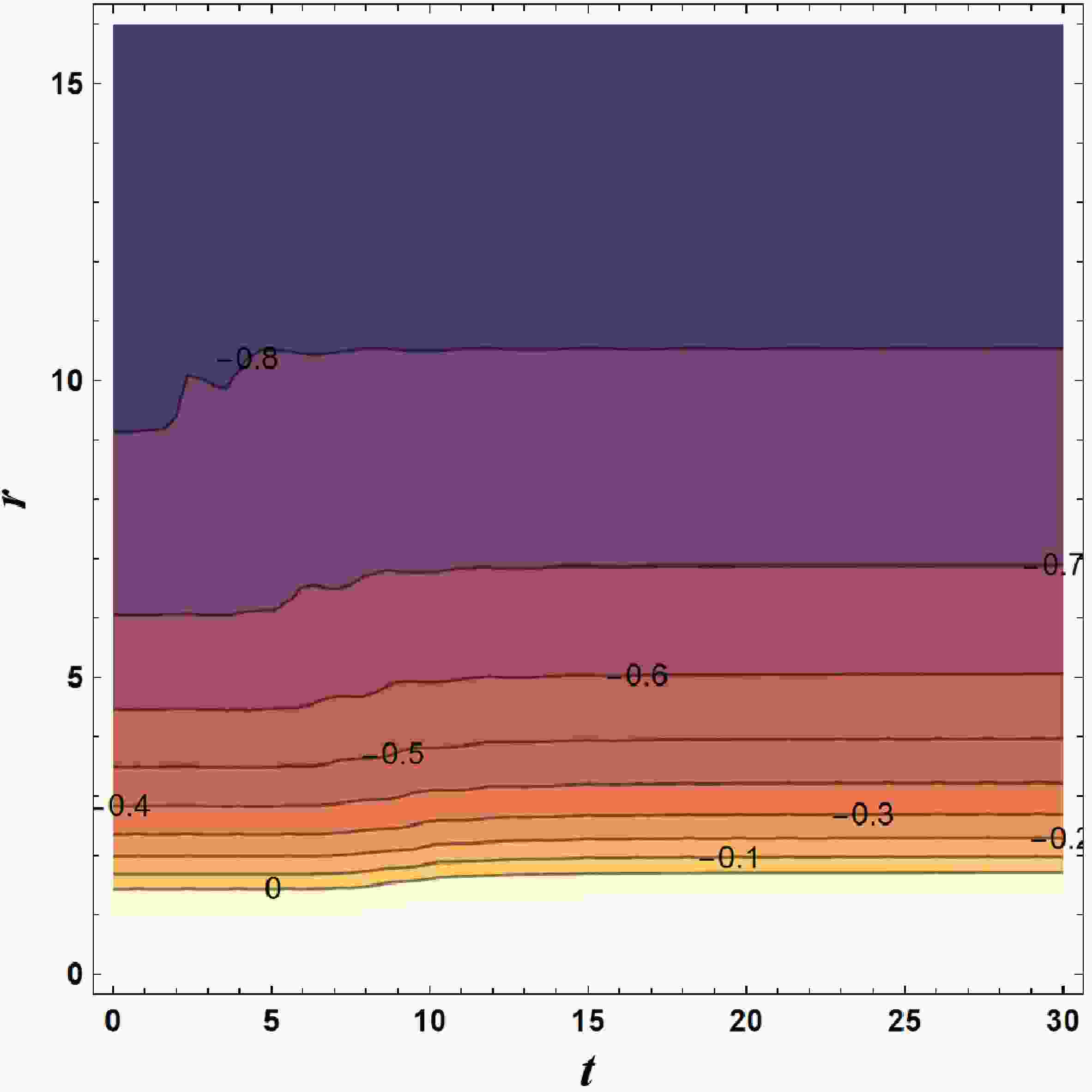
$ \psi(t,r) $ , gauge potential$ A(t,r) $ , and metric {$ \alpha(t,r), \zeta(t,r) $ } over all positions (r) and all times (t). In this study, we set the potential$ V(\psi)=|\psi|^{2}(1-\dfrac{|\psi|^{2}}{0.1^{2}})^{2}, M= 1.09239 $ , the total charge$ Q=0.9 $ , and$ q=3 $ .Figure 1 illustrates the contour plot of the metric component
$ g_{tt} $ as a function of time t and radial coordinate r. The contour line of$ g_{tt}=0 $ corresponds to the location of the apparent horizon$ r_{\rm h} $ , which increases with time t.$ g_{tt} $ shows little variation with t and asymptotically approaches$ -1 $ as r tends to infinity. Figure 2 displays a contour plot of$ g_{tr} $ as a function of t and r.$ g_{tr} $ also shows little variation with t and asymptotically approaches 0 as r tends to infinity. The metric of this dynamic black hole describes an asymptotically flat spacetime. The complex scalar field$ \psi(t, r) $ of this black hole is a function of t and r. Figure 3 depicts how the magnitude of the complex scalar field on the horizon$ |\psi_{\rm h}| $ changes with time. Initially,$ |\psi_{\rm h}|=0 $ , and at this point, the black hole has not yet acquired scalar hair. Then, there is a sharp rise followed by rapid oscillations. As time progresses, the oscillations gradually dampen, and then, the magnitude tends toward stabilization.
Figure 1. (color online) Contour plot of
$ g_{tt} $ as a function of time t and radial coordinate r. This parameter asymptotically approaches$ -1 $ as$ r\rightarrow \infty $ . The contour line of$ g_{tt}=0 $ corresponds to the position of the apparent horizon$ r_{\rm h} $ .
Figure 2. (color online) Contour plot of
$ g_{tr} $ as a function of time t and radial coordinate r. This parameter asymptotically approaches 0 as$ r\rightarrow \infty $ .
Figure 3. Variation in the magnitude of the complex scalar field on the horizon
$ |\psi_{\rm h}| $ with time t.The Lagrangian
$ {\cal{L}} $ of photon propagation in the spacetime can be characterized by$ \begin{aligned}[b]{\cal{L}}=\;&\frac{1}{2} g_{\mu\nu}\dot{x}^{\mu}\dot{x}^{\nu}=\frac{1}{2}[-(1-\zeta^{2})\alpha^{2}\dot{t}^{2}+2\alpha\zeta \dot{t}\dot{r}+\dot{r}^{2}\\&+r^{2}(\dot{\theta}^{2}+\sin^{2}\theta \dot{\phi}^{2})]=0. \end{aligned}$
(18) As the variable
$ \phi $ is not present in$ {\cal{L}} $ ,$ p_{\phi} $ is a conserved quantity in the motions of photons and can be expressed as angular momentum$ L=p_{\phi}=\frac{\partial{\cal{L}}}{\partial\dot{\phi}}=r^{2}\sin^{2}\theta \dot{\phi}. $
(19) As the spacetime is spherically symmetric, without any loss of generality, we investigate the photon motion in the plane
$ \theta=\pi/2 $ . The Lagrangian$ {\cal{L}} $ (18) can be rewritten as$ {\cal{L}}=\frac{1}{2}[-(1-\zeta^{2})\alpha^{2}\dot{t}^{2}+2\alpha\zeta \dot{t}\dot{r}+\dot{r}^{2}+r^{2}\dot{\phi}^{2}]=0. $
(20) The photon sphere is closely associated with the shadows of black holes, satisfying
$ \dot{r}=0\;\;\;\;\;\;\; {\rm and} \;\;\;\;\;\;\;\ddot{r}=0, $
(21) where the dot
$ \cdot $ denotes the derivative with respect to the affine parameter. According to$ {\cal{L}}=0 $ (20) and$ \dot{r}=0 $ , one can obtain$ -(1-\zeta^{2})\alpha^{2}\dot{t}^{2}+r^{2}\dot{\phi}^{2}=-(1-\zeta^{2})\alpha^{2}\dot{t}^{2}+\frac{L^{2}}{r^{2}}=0. $
(22) The equations of geodesic motion in this spacetime are
$\begin{aligned}[b] \ddot{t}=\;&-\left(\frac{1}{2}g^{tt}g_{tt,t}+\frac{1}{2}g^{tr}\left(2g_{tr,t}-g_{tt,r}\right)\right)\dot{t}^{2}-g^{tt}g_{tt,r}\dot{t}\dot{r}\\&-g^{tt}g_{tr,r}\dot{r}^{2}+g^{tr}r\dot{\theta}^{2}+g^{tr}\frac{L^{2}}{r^{3}\sin^{2}\theta},\end{aligned} $
(23) $\begin{aligned}[b] \ddot{r}=\;&-\left(\frac{1}{2}g^{tr}g_{tt,t}+g_{tr,t}-\frac{1}{2}g_{tt,r}\right)\dot{t}^{2}-g^{tr}g_{tt,r}\dot{t}\dot{r}\\&-g^{tr}g_{tr,r}\dot{r}^{2}+r\dot{\theta}^{2}+\frac{L^{2}}{r^{3}\sin^{2}\theta},\end{aligned} $
(24) $ \ddot{\theta}=\frac{L^{2}\cos\theta}{r^{4}\sin^{3}\theta}-2\frac{1}{r}\dot{r}\dot{\theta}, $
(25) $ \dot{\phi}=\frac{L}{r^{2}\sin^{2}\theta} . $
(26) The radius of the photon sphere
$ r_{\rm ps} $ can be determined by solving the combined conditions derived from Eqs. (21), (22), and (24), which require that$ r_{\rm ps} $ satisfies$ g^{tr}g_{tt,t}+2g_{tr,t}-g_{tt,r}+\frac{1}{r}g_{tt}=0. $
(27) Figure 4 illustrates the variations in photon sphere radius
$ r_{\rm ps} $ (marked by a red solid line) and the apparent horizon radius$ r_{\rm h} $ (marked by a black dashed line) with respect to time t. The radius of the photon sphere$ r_{\rm ps} $ remains constant initially, then experiences a significant and rapid increase subsequently, followed by some fluctuations, and finally stabilizes. The variation in the photon sphere radius$ r_{\rm ps} $ exhibits a striking similarity to that of the magnitude$ |\psi_{\rm h}| $ as illustrated in Fig. 3. The complex scalar field$ \psi $ is capable of inducing a variation in the photon sphere radius$ r_{\rm ps} $ . Moreover, it will give rise to a dynamically evolving black hole shadow and endow it with new features. The radius of the apparent horizon$ r_{\rm h} $ also remains constant initially, then increases rapidly, and smoothly approaches a stable value eventually. The appearance of the complex scalar hair$ \psi $ causes an increase in the apparent horizon$ r_{\rm h} $ .
Figure 4. (color online) Variations in the apparent horizon
$ r_{\rm h} $ (marked by a black dashed line) and photon sphere$ r_{\rm ps} $ (marked by a red solid line) with respect to the variable t. -
The black hole spacetime we consider is the Einstein-Maxwell gravity minimally coupled with a self-interacting massive complex scalar
$ \psi $ [59]. The Lagrangian density is$ {\cal{L}}=R-F_{\mu\nu}F^{\mu\nu}-D^{\mu}\psi(D_{}\psi)^{\ast}-V(\psi). $
(1) $ F_{\mu\nu}=\partial_{\mu}A_{\nu}-\partial_{\nu}A_{\mu} $ is the Maxwell field strength, where$ A_{\mu} $ is the gauge potential. The gauge covariant derivative is defined as$ D_{\mu}=\nabla_{\mu}-{\rm i}q A_{\mu} $ , where q denotes the gauge coupling constant of the complex scalar field$ \psi $ . The potential is given by$ V(\psi)=\mu^{2}|\psi|^{2}-\lambda|\psi|^{4}+\nu|\psi|^{6} $ , where$ \mu $ is the scalar field mass, and$ \lambda, \nu $ are positive self-interaction parameters [59]. The Einstein equations are given as$ R_{\mu\nu}-\frac{1}{2}g_{\mu\nu}R=2T^{A}_{\mu\nu}+T^{\psi}_{\mu\nu}, $
(2) where the energy-momentum tensors are
$ T^{A}_{\mu\nu}=F_{\mu\rho}F_{\nu}^{\rho}-\frac{1}{4}g_{\mu\nu}F_{\rho\sigma}F^{\rho\sigma}, $
(3) $\begin{aligned}[b] T^{\psi}_{\mu\nu}=\;&\frac{1}{2}(D_{\mu}\psi)^{\ast}(D_{\nu}\psi)+\frac{1}{2}(D_{\mu}\psi)(D_{\nu}\psi)^{\ast}\\&+\frac{1}{2}g_{\mu\nu}(D^{\mu}\psi(D_{\mu}\psi)^{\ast}+V).\end{aligned} $
(4) The Maxwell equations are written as
$ \nabla_{\mu}F^{\mu\nu}=\frac{1}{4}{\rm i} q[\psi^{\ast}\nabla_{\mu}\psi-\psi(\nabla_{\mu}\psi)^{\ast}]g^{\mu\nu}. $
(5) The scalar equation is written as
$ D^{\mu}D_{\mu}\psi=\frac{\partial V}{\partial|\psi|^{2}}\psi. $
(6) The dynamic black hole with the self-interacting massive complex scalar hair in the
$\mathrm{Painlev \acute{e}} $ -Gullstrand (PG) coordinates is expressed as follows:$\begin{aligned}[b] {\rm d}s^{2}=\;&-[1-\zeta(t,r)^{2}]\alpha(t,r)^{2}{\rm d}t^{2}+2\alpha(t,r)\zeta(t,r) {\rm d}t{\rm d}r\\&+{\rm d}r^{2}+r^{2}({\rm d}\theta^{2}+\sin^{2}\theta {\rm d}\phi^{2}).\end{aligned} $
(7) Here,
$ \alpha, \zeta $ are metric functions dependent on t and r. This coordinate system remains regular at the apparent horizon$ r_{\rm h} $ where$ \zeta(t, r_{\rm h})=1 $ . The gauge potential$ A_{\mu}{\rm d}x^{\mu}=A{\rm d}t $ . Introducing auxiliary variables [59]$ \Phi=\partial_{r}\psi, $
(8) $ \Pi=\frac{1}{\alpha}(\partial_{t}\psi-{\rm i}qA\psi)-\zeta\Phi, $
(9) $ B=\frac{1}{\alpha}\partial_{r}A. $
(10) The Einstein equations can be reduced to
$ 0=\partial_{r}\alpha+\frac{\alpha r \mathrm{Re}(\Pi\Phi^{\ast})}{2\zeta}, $
(11) $ 0=\partial_{r}\zeta+\frac{\zeta}{2r}-\frac{r}{4\zeta}(\Pi\Pi^{\ast}+\Phi\Phi^{\ast}+2B^{2}+V)-\frac{r}{2}\mathrm{Re}(\Pi\Phi^{\ast}), $
(12) $ 0=\partial_{t}\zeta-\frac{1}{2}\alpha r\bigg[\Pi\Pi^{\ast}+\Phi\Phi^{\ast}+\bigg(\zeta+\frac{1}{\zeta}\bigg)\mathrm{Re}(\Pi\Phi^{\ast})\bigg]. $
(13) The Maxwell equations are expressed as
$ 0=\partial_{r}B+\frac{2B}{r}-\frac{q}{2}\mathrm{Im}(\Pi\Phi^{\ast}), $
(14) $ 0=\partial_{t}B-\frac{q}{2}\alpha\mathrm{Im}[(\zeta\Pi+\Phi)\psi^{\ast}]. $
(15) The scalar equation becomes
$ 0=\partial_{t}\Pi-\partial_{r}[\alpha(\Pi\zeta+\Phi)]-\frac{2\alpha(\Pi\zeta+\Phi)}{r}-{\rm i}A\Pi q+\alpha\psi\frac{\partial V}{\partial|\psi|^{2}}. $
(16) At asymptotic spatial infinity, we have
$ \zeta=\sqrt{\frac{2M}{r}\left[1+O\left(\frac{1}{r}\right)\right]}, $
(17) where M is the total mass. By numerically solving the above equations, we can obtain the complex scalar field
$ \psi(t,r) $ , gauge potential$ A(t,r) $ , and metric {$ \alpha(t,r), \zeta(t,r) $ } over all positions (r) and all times (t). In this study, we set the potential$ V(\psi)=|\psi|^{2}(1-\dfrac{|\psi|^{2}}{0.1^{2}})^{2}, M= 1.09239 $ , the total charge$ Q=0.9 $ , and$ q=3 $ .Figure 1 illustrates the contour plot of the metric component
$ g_{tt} $ as a function of time t and radial coordinate r. The contour line of$ g_{tt}=0 $ corresponds to the location of the apparent horizon$ r_{\rm h} $ , which increases with time t.$ g_{tt} $ shows little variation with t and asymptotically approaches$ -1 $ as r tends to infinity. Figure 2 displays a contour plot of$ g_{tr} $ as a function of t and r.$ g_{tr} $ also shows little variation with t and asymptotically approaches 0 as r tends to infinity. The metric of this dynamic black hole describes an asymptotically flat spacetime. The complex scalar field$ \psi(t, r) $ of this black hole is a function of t and r. Figure 3 depicts how the magnitude of the complex scalar field on the horizon$ |\psi_{\rm h}| $ changes with time. Initially,$ |\psi_{\rm h}|=0 $ , and at this point, the black hole has not yet acquired scalar hair. Then, there is a sharp rise followed by rapid oscillations. As time progresses, the oscillations gradually dampen, and then, the magnitude tends toward stabilization.
Figure 1. (color online) Contour plot of
$ g_{tt} $ as a function of time t and radial coordinate r. This parameter asymptotically approaches$ -1 $ as$ r\rightarrow \infty $ . The contour line of$ g_{tt}=0 $ corresponds to the position of the apparent horizon$ r_{\rm h} $ .
Figure 2. (color online) Contour plot of
$ g_{tr} $ as a function of time t and radial coordinate r. This parameter asymptotically approaches 0 as$ r\rightarrow \infty $ .
Figure 3. Variation in the magnitude of the complex scalar field on the horizon
$ |\psi_{\rm h}| $ with time t.The Lagrangian
$ {\cal{L}} $ of photon propagation in the spacetime can be characterized by$ \begin{aligned}[b]{\cal{L}}=\;&\frac{1}{2} g_{\mu\nu}\dot{x}^{\mu}\dot{x}^{\nu}=\frac{1}{2}[-(1-\zeta^{2})\alpha^{2}\dot{t}^{2}+2\alpha\zeta \dot{t}\dot{r}+\dot{r}^{2}\\&+r^{2}(\dot{\theta}^{2}+\sin^{2}\theta \dot{\phi}^{2})]=0. \end{aligned}$
(18) As the variable
$ \phi $ is not present in$ {\cal{L}} $ ,$ p_{\phi} $ is a conserved quantity in the motions of photons and can be expressed as angular momentum$ L=p_{\phi}=\frac{\partial{\cal{L}}}{\partial\dot{\phi}}=r^{2}\sin^{2}\theta \dot{\phi}. $
(19) As the spacetime is spherically symmetric, without any loss of generality, we investigate the photon motion in the plane
$ \theta=\pi/2 $ . The Lagrangian$ {\cal{L}} $ (18) can be rewritten as$ {\cal{L}}=\frac{1}{2}[-(1-\zeta^{2})\alpha^{2}\dot{t}^{2}+2\alpha\zeta \dot{t}\dot{r}+\dot{r}^{2}+r^{2}\dot{\phi}^{2}]=0. $
(20) The photon sphere is closely associated with the shadows of black holes, satisfying
$ \dot{r}=0\;\;\;\;\;\;\; {\rm and} \;\;\;\;\;\;\;\ddot{r}=0, $
(21) where the dot
$ \cdot $ denotes the derivative with respect to the affine parameter. According to$ {\cal{L}}=0 $ (20) and$ \dot{r}=0 $ , one can obtain$ -(1-\zeta^{2})\alpha^{2}\dot{t}^{2}+r^{2}\dot{\phi}^{2}=-(1-\zeta^{2})\alpha^{2}\dot{t}^{2}+\frac{L^{2}}{r^{2}}=0. $
(22) The equations of geodesic motion in this spacetime are
$\begin{aligned}[b] \ddot{t}=\;&-\left(\frac{1}{2}g^{tt}g_{tt,t}+\frac{1}{2}g^{tr}\left(2g_{tr,t}-g_{tt,r}\right)\right)\dot{t}^{2}-g^{tt}g_{tt,r}\dot{t}\dot{r}\\&-g^{tt}g_{tr,r}\dot{r}^{2}+g^{tr}r\dot{\theta}^{2}+g^{tr}\frac{L^{2}}{r^{3}\sin^{2}\theta},\end{aligned} $
(23) $\begin{aligned}[b] \ddot{r}=\;&-\left(\frac{1}{2}g^{tr}g_{tt,t}+g_{tr,t}-\frac{1}{2}g_{tt,r}\right)\dot{t}^{2}-g^{tr}g_{tt,r}\dot{t}\dot{r}\\&-g^{tr}g_{tr,r}\dot{r}^{2}+r\dot{\theta}^{2}+\frac{L^{2}}{r^{3}\sin^{2}\theta},\end{aligned} $
(24) $ \ddot{\theta}=\frac{L^{2}\cos\theta}{r^{4}\sin^{3}\theta}-2\frac{1}{r}\dot{r}\dot{\theta}, $
(25) $ \dot{\phi}=\frac{L}{r^{2}\sin^{2}\theta} . $
(26) The radius of the photon sphere
$ r_{\rm ps} $ can be determined by solving the combined conditions derived from Eqs. (21), (22), and (24), which require that$ r_{\rm ps} $ satisfies$ g^{tr}g_{tt,t}+2g_{tr,t}-g_{tt,r}+\frac{1}{r}g_{tt}=0. $
(27) Figure 4 illustrates the variations in photon sphere radius
$ r_{\rm ps} $ (marked by a red solid line) and the apparent horizon radius$ r_{\rm h} $ (marked by a black dashed line) with respect to time t. The radius of the photon sphere$ r_{\rm ps} $ remains constant initially, then experiences a significant and rapid increase subsequently, followed by some fluctuations, and finally stabilizes. The variation in the photon sphere radius$ r_{\rm ps} $ exhibits a striking similarity to that of the magnitude$ |\psi_{\rm h}| $ as illustrated in Fig. 3. The complex scalar field$ \psi $ is capable of inducing a variation in the photon sphere radius$ r_{\rm ps} $ . Moreover, it will give rise to a dynamically evolving black hole shadow and endow it with new features. The radius of the apparent horizon$ r_{\rm h} $ also remains constant initially, then increases rapidly, and smoothly approaches a stable value eventually. The appearance of the complex scalar hair$ \psi $ causes an increase in the apparent horizon$ r_{\rm h} $ .
Figure 4. (color online) Variations in the apparent horizon
$ r_{\rm h} $ (marked by a black dashed line) and photon sphere$ r_{\rm ps} $ (marked by a red solid line) with respect to the variable t. -
The black hole spacetime we consider is the Einstein-Maxwell gravity minimally coupled with a self-interacting massive complex scalar
$ \psi $ [59]. The Lagrangian density is$ {\cal{L}}=R-F_{\mu\nu}F^{\mu\nu}-D^{\mu}\psi(D_{}\psi)^{\ast}-V(\psi). $

(1) $ F_{\mu\nu}=\partial_{\mu}A_{\nu}-\partial_{\nu}A_{\mu} $ is the Maxwell field strength, where$ A_{\mu} $ is the gauge potential. The gauge covariant derivative is defined as$ D_{\mu}=\nabla_{\mu}-{\rm i}q A_{\mu} $ , where q denotes the gauge coupling constant of the complex scalar field$ \psi $ . The potential is given by$ V(\psi)=\mu^{2}|\psi|^{2}-\lambda|\psi|^{4}+\nu|\psi|^{6} $ , where$ \mu $ is the scalar field mass, and$ \lambda, \nu $ are positive self-interaction parameters [59]. The Einstein equations are given as$ R_{\mu\nu}-\frac{1}{2}g_{\mu\nu}R=2T^{A}_{\mu\nu}+T^{\psi}_{\mu\nu}, $

(2) where the energy-momentum tensors are
$ T^{A}_{\mu\nu}=F_{\mu\rho}F_{\nu}^{\rho}-\frac{1}{4}g_{\mu\nu}F_{\rho\sigma}F^{\rho\sigma}, $

(3) $\begin{aligned}[b] T^{\psi}_{\mu\nu}=\;&\frac{1}{2}(D_{\mu}\psi)^{\ast}(D_{\nu}\psi)+\frac{1}{2}(D_{\mu}\psi)(D_{\nu}\psi)^{\ast}\\&+\frac{1}{2}g_{\mu\nu}(D^{\mu}\psi(D_{\mu}\psi)^{\ast}+V).\end{aligned} $

(4) The Maxwell equations are written as
$ \nabla_{\mu}F^{\mu\nu}=\frac{1}{4}{\rm i} q[\psi^{\ast}\nabla_{\mu}\psi-\psi(\nabla_{\mu}\psi)^{\ast}]g^{\mu\nu}. $

(5) The scalar equation is written as
$ D^{\mu}D_{\mu}\psi=\frac{\partial V}{\partial|\psi|^{2}}\psi. $

(6) The dynamic black hole with the self-interacting massive complex scalar hair in the
$\mathrm{Painlev \acute{e}} $ -Gullstrand (PG) coordinates is expressed as follows:$\begin{aligned}[b] {\rm d}s^{2}=\;&-[1-\zeta(t,r)^{2}]\alpha(t,r)^{2}{\rm d}t^{2}+2\alpha(t,r)\zeta(t,r) {\rm d}t{\rm d}r\\&+{\rm d}r^{2}+r^{2}({\rm d}\theta^{2}+\sin^{2}\theta {\rm d}\phi^{2}).\end{aligned} $

(7) Here,
$ \alpha, \zeta $ are metric functions dependent on t and r. This coordinate system remains regular at the apparent horizon$ r_{\rm h} $ where$ \zeta(t, r_{\rm h})=1 $ . The gauge potential$ A_{\mu}{\rm d}x^{\mu}=A{\rm d}t $ . Introducing auxiliary variables [59]$ \Phi=\partial_{r}\psi, $

(8) $ \Pi=\frac{1}{\alpha}(\partial_{t}\psi-{\rm i}qA\psi)-\zeta\Phi, $

(9) $ B=\frac{1}{\alpha}\partial_{r}A. $

(10) The Einstein equations can be reduced to
$ 0=\partial_{r}\alpha+\frac{\alpha r \mathrm{Re}(\Pi\Phi^{\ast})}{2\zeta}, $

(11) $ 0=\partial_{r}\zeta+\frac{\zeta}{2r}-\frac{r}{4\zeta}(\Pi\Pi^{\ast}+\Phi\Phi^{\ast}+2B^{2}+V)-\frac{r}{2}\mathrm{Re}(\Pi\Phi^{\ast}), $

(12) $ 0=\partial_{t}\zeta-\frac{1}{2}\alpha r\bigg[\Pi\Pi^{\ast}+\Phi\Phi^{\ast}+\bigg(\zeta+\frac{1}{\zeta}\bigg)\mathrm{Re}(\Pi\Phi^{\ast})\bigg]. $

(13) The Maxwell equations are expressed as
$ 0=\partial_{r}B+\frac{2B}{r}-\frac{q}{2}\mathrm{Im}(\Pi\Phi^{\ast}), $

(14) $ 0=\partial_{t}B-\frac{q}{2}\alpha\mathrm{Im}[(\zeta\Pi+\Phi)\psi^{\ast}]. $

(15) The scalar equation becomes
$ 0=\partial_{t}\Pi-\partial_{r}[\alpha(\Pi\zeta+\Phi)]-\frac{2\alpha(\Pi\zeta+\Phi)}{r}-{\rm i}A\Pi q+\alpha\psi\frac{\partial V}{\partial|\psi|^{2}}. $

(16) At asymptotic spatial infinity, we have
$ \zeta=\sqrt{\frac{2M}{r}\left[1+O\left(\frac{1}{r}\right)\right]}, $

(17) where M is the total mass. By numerically solving the above equations, we can obtain the complex scalar field
$ \psi(t,r) $ , gauge potential$ A(t,r) $ , and metric {$ \alpha(t,r), \zeta(t,r) $ } over all positions (r) and all times (t). In this study, we set the potential$ V(\psi)=|\psi|^{2}(1-\dfrac{|\psi|^{2}}{0.1^{2}})^{2}, M= 1.09239 $ , the total charge$ Q=0.9 $ , and$ q=3 $ .Figure 1 illustrates the contour plot of the metric component
$ g_{tt} $ as a function of time t and radial coordinate r. The contour line of$ g_{tt}=0 $ corresponds to the location of the apparent horizon$ r_{\rm h} $ , which increases with time t.$ g_{tt} $ shows little variation with t and asymptotically approaches$ -1 $ as r tends to infinity. Figure 2 displays a contour plot of$ g_{tr} $ as a function of t and r.$ g_{tr} $ also shows little variation with t and asymptotically approaches 0 as r tends to infinity. The metric of this dynamic black hole describes an asymptotically flat spacetime. The complex scalar field$ \psi(t, r) $ of this black hole is a function of t and r. Figure 3 depicts how the magnitude of the complex scalar field on the horizon$ |\psi_{\rm h}| $ changes with time. Initially,$ |\psi_{\rm h}|=0 $ , and at this point, the black hole has not yet acquired scalar hair. Then, there is a sharp rise followed by rapid oscillations. As time progresses, the oscillations gradually dampen, and then, the magnitude tends toward stabilization.
Figure 1. (color online) Contour plot of
$ g_{tt} $ as a function of time t and radial coordinate r. This parameter asymptotically approaches$ -1 $ as$ r\rightarrow \infty $ . The contour line of$ g_{tt}=0 $ corresponds to the position of the apparent horizon$ r_{\rm h} $ .
Figure 2. (color online) Contour plot of
$ g_{tr} $ as a function of time t and radial coordinate r. This parameter asymptotically approaches 0 as$ r\rightarrow \infty $ .
Figure 3. Variation in the magnitude of the complex scalar field on the horizon
$ |\psi_{\rm h}| $ with time t.The Lagrangian
$ {\cal{L}} $ of photon propagation in the spacetime can be characterized by$ \begin{aligned}[b]{\cal{L}}=\;&\frac{1}{2} g_{\mu\nu}\dot{x}^{\mu}\dot{x}^{\nu}=\frac{1}{2}[-(1-\zeta^{2})\alpha^{2}\dot{t}^{2}+2\alpha\zeta \dot{t}\dot{r}+\dot{r}^{2}\\&+r^{2}(\dot{\theta}^{2}+\sin^{2}\theta \dot{\phi}^{2})]=0. \end{aligned}$

(18) As the variable
$ \phi $ is not present in$ {\cal{L}} $ ,$ p_{\phi} $ is a conserved quantity in the motions of photons and can be expressed as angular momentum$ L=p_{\phi}=\frac{\partial{\cal{L}}}{\partial\dot{\phi}}=r^{2}\sin^{2}\theta \dot{\phi}. $

(19) As the spacetime is spherically symmetric, without any loss of generality, we investigate the photon motion in the plane
$ \theta=\pi/2 $ . The Lagrangian$ {\cal{L}} $ (18) can be rewritten as$ {\cal{L}}=\frac{1}{2}[-(1-\zeta^{2})\alpha^{2}\dot{t}^{2}+2\alpha\zeta \dot{t}\dot{r}+\dot{r}^{2}+r^{2}\dot{\phi}^{2}]=0. $

(20) The photon sphere is closely associated with the shadows of black holes, satisfying
$ \dot{r}=0\;\;\;\;\;\;\; {\rm and} \;\;\;\;\;\;\;\ddot{r}=0, $

(21) where the dot
$ \cdot $ denotes the derivative with respect to the affine parameter. According to$ {\cal{L}}=0 $ (20) and$ \dot{r}=0 $ , one can obtain$ -(1-\zeta^{2})\alpha^{2}\dot{t}^{2}+r^{2}\dot{\phi}^{2}=-(1-\zeta^{2})\alpha^{2}\dot{t}^{2}+\frac{L^{2}}{r^{2}}=0. $

(22) The equations of geodesic motion in this spacetime are
$\begin{aligned}[b] \ddot{t}=\;&-\left(\frac{1}{2}g^{tt}g_{tt,t}+\frac{1}{2}g^{tr}\left(2g_{tr,t}-g_{tt,r}\right)\right)\dot{t}^{2}-g^{tt}g_{tt,r}\dot{t}\dot{r}\\&-g^{tt}g_{tr,r}\dot{r}^{2}+g^{tr}r\dot{\theta}^{2}+g^{tr}\frac{L^{2}}{r^{3}\sin^{2}\theta},\end{aligned} $

(23) $\begin{aligned}[b] \ddot{r}=\;&-\left(\frac{1}{2}g^{tr}g_{tt,t}+g_{tr,t}-\frac{1}{2}g_{tt,r}\right)\dot{t}^{2}-g^{tr}g_{tt,r}\dot{t}\dot{r}\\&-g^{tr}g_{tr,r}\dot{r}^{2}+r\dot{\theta}^{2}+\frac{L^{2}}{r^{3}\sin^{2}\theta},\end{aligned} $

(24) $ \ddot{\theta}=\frac{L^{2}\cos\theta}{r^{4}\sin^{3}\theta}-2\frac{1}{r}\dot{r}\dot{\theta}, $

(25) $ \dot{\phi}=\frac{L}{r^{2}\sin^{2}\theta} . $

(26) The radius of the photon sphere
$ r_{\rm ps} $ can be determined by solving the combined conditions derived from Eqs. (21), (22), and (24), which require that$ r_{\rm ps} $ satisfies$ g^{tr}g_{tt,t}+2g_{tr,t}-g_{tt,r}+\frac{1}{r}g_{tt}=0. $

(27) Figure 4 illustrates the variations in photon sphere radius
$ r_{\rm ps} $ (marked by a red solid line) and the apparent horizon radius$ r_{\rm h} $ (marked by a black dashed line) with respect to time t. The radius of the photon sphere$ r_{\rm ps} $ remains constant initially, then experiences a significant and rapid increase subsequently, followed by some fluctuations, and finally stabilizes. The variation in the photon sphere radius$ r_{\rm ps} $ exhibits a striking similarity to that of the magnitude$ |\psi_{\rm h}| $ as illustrated in Fig. 3. The complex scalar field$ \psi $ is capable of inducing a variation in the photon sphere radius$ r_{\rm ps} $ . Moreover, it will give rise to a dynamically evolving black hole shadow and endow it with new features. The radius of the apparent horizon$ r_{\rm h} $ also remains constant initially, then increases rapidly, and smoothly approaches a stable value eventually. The appearance of the complex scalar hair$ \psi $ causes an increase in the apparent horizon$ r_{\rm h} $ .
Figure 4. (color online) Variations in the apparent horizon
$ r_{\rm h} $ (marked by a black dashed line) and photon sphere$ r_{\rm ps} $ (marked by a red solid line) with respect to the variable t. -
The black hole spacetime we consider is the Einstein-Maxwell gravity minimally coupled with a self-interacting massive complex scalar
$ \psi $ [59]. The Lagrangian density is$ {\cal{L}}=R-F_{\mu\nu}F^{\mu\nu}-D^{\mu}\psi(D_{}\psi)^{\ast}-V(\psi). $
(1) $ F_{\mu\nu}=\partial_{\mu}A_{\nu}-\partial_{\nu}A_{\mu} $ is the Maxwell field strength with$ A_{\mu} $ is the gauge potential. The gauge covariant derivative is defined as$ D_{\mu}=\nabla_{\mu}-iq A_{\mu} $ , where q denotes the gauge coupling constant of the complex scalar field$ \psi $ . The potential is given by$ V(\psi)=\mu^{2}|\psi|^{2}-\lambda|\psi|^{4}+\nu|\psi|^{6} $ , with$ \mu $ as the scalar field mass, and$ \lambda, \nu $ as positive self-interaction parameters[59]. The Einstein equations are given as$ R_{\mu\nu}-\frac{1}{2}g_{\mu\nu}R=2T^{A}_{\mu\nu}+T^{\psi}_{\mu\nu}, $
(2) where the energy-momentum tensors are
$ T^{A}_{\mu\nu}=F_{\mu\rho}F_{\nu}^{\rho}-\frac{1}{4}g_{\mu\nu}F_{\rho\sigma}F^{\rho\sigma}, $
(3) $\begin{aligned}[b] T^{\psi}_{\mu\nu}=\;&\frac{1}{2}(D_{\mu}\psi)^{\ast}(D_{\nu}\psi)+\frac{1}{2}(D_{\mu}\psi)(D_{\nu}\psi)^{\ast}\\&+\frac{1}{2}g_{\mu\nu}(D^{\mu}\psi(D_{\mu}\psi)^{\ast}+V).\end{aligned} $
(4) The Maxwell equations are written as
$ \nabla_{\mu}F^{\mu\nu}=\frac{1}{4}iq[\psi^{\ast}\nabla_{\mu}\psi-\psi(\nabla_{\mu}\psi)^{\ast}]g^{\mu\nu}. $
(5) The scalar equation is written as
$ D^{\mu}D_{\mu}\psi=\frac{\partial V}{\partial|\psi|^{2}}\psi. $
(6) The dynamic black hole with the self-interacting massive complex scalar hair in the Painlev
$ \acute{e} $ -Gullstrand (PG) coordinates is described as follows:$\begin{aligned}[b] ds^{2}=\;&-[1-\zeta(t,r)^{2}]\alpha(t,r)^{2}dt^{2}+2\alpha(t,r)\zeta(t,r) dtdr\\&+dr^{2}+r^{2}(d\theta^{2}+\sin^{2}\theta d\phi^{2}).\end{aligned} $
(7) Here
$ \alpha, \zeta $ are metric functions dependent on t and r. This coordinate system remains regular at the apparent horizon$ r_{h} $ where$ \zeta(t, r_{h})=1 $ . The gauge potential$ A_{\mu}dx^{\mu}=Adt $ . Introducing auxiliary variables[59]$ \Phi=\partial_{r}\psi, $
(8) $ \Pi=\frac{1}{\alpha}(\partial_{t}\psi-iqA\psi)-\zeta\Phi, $
(9) $ B=\frac{1}{\alpha}\partial_{r}A. $
(10) The Einstein equations can be reduced to
$ 0=\partial_{r}\alpha+\frac{\alpha r \mathrm{Re}(\Pi\Phi^{\ast})}{2\zeta}, $
(11) $ 0=\partial_{r}\zeta+\frac{\zeta}{2r}-\frac{r}{4\zeta}(\Pi\Pi^{\ast}+\Phi\Phi^{\ast}+2B^{2}+V)-\frac{r}{2}\mathrm{Re}(\Pi\Phi^{\ast}), $
(12) $ 0=\partial_{t}\zeta-\frac{1}{2}\alpha r\bigg[\Pi\Pi^{\ast}+\Phi\Phi^{\ast}+\bigg(\zeta+\frac{1}{\zeta}\bigg)\mathrm{Re}(\Pi\Phi^{\ast})\bigg]. $
(13) The Maxwell equations are give as
$ 0=\partial_{r}B+\frac{2B}{r}-\frac{q}{2}\mathrm{Im}(\Pi\Phi^{\ast}), $
(14) $ 0=\partial_{t}B-\frac{q}{2}\alpha\mathrm{Im}[(\zeta\Pi+\Phi)\psi^{\ast}]. $
(15) The scalar equation becomes
$ 0=\partial_{t}\Pi-\partial_{r}[\alpha(\Pi\zeta+\Phi)]-\frac{2\alpha(\Pi\zeta+\Phi)}{r}-iA\Pi q+\alpha\psi\frac{\partial V}{\partial|\psi|^{2}}. $
(16) At asymptotic spatial infinity, there are
$ \zeta=\sqrt{\frac{2M}{r}\left[1+O\left(\frac{1}{r}\right)\right]}, $
(17) where M is the total mass. By numerically solving the above equations, we can obtain the complex scalar field
$ \psi(t,r) $ , the gauge potential$ A(t,r) $ , and metric {$ \alpha(t,r), \zeta(t,r) $ } over all positions (r) and all times (t). In this paper, we set the potential$ V(\psi)=|\psi|^{2}(1-\dfrac{|\psi|^{2}}{0.1^{2}})^{2}, M=1.09239 $ , the total charge$ Q=0.9 $ , and$ q=3 $ .Figure 1 illustrates the contour plot of the metric component
$ g_{tt} $ as functions of time t and radial coordinate r. The contour line of$ g_{tt}=0 $ corresponds to the location of the apparent horizon$ r_{h} $ , which increases with time t. The$ g_{tt} $ has little variation with t and asymptotically approaches$ -1 $ as r tends to infinity. Figure 2 displays a contour plot of$ g_{tr} $ as a function of t and r. The$ g_{tr} $ also has little variation with t and asymptotically approaches 0 as r tends to infinity. The metric of this dynamic black hole describes an asymptotically flat spacetime. The complex scalar field$ \psi(t, r) $ of this black hole is a function of t and r. Figure 3 depicts how the magnitude of the complex scalar field on the horizon$ |\psi_{h}| $ changes over time. Initially,$ |\psi_{h}|=0 $ , and at this point, the black hole has not yet acquired scalar hair. Then there is a sharp rise followed by rapid oscillations. As time progresses, the oscillation gradually dampen, and then the magnitude tends toward stabilization.
Figure 1. (color online) The contour plot of
$ g_{tt} $ as a function of time t and radial coordinate r, which asymptotically approaches$ -1 $ as$ r\rightarrow \infty $ . The contour line of$ g_{tt}=0 $ corresponds to the position of apparent horizon$ r_{h} $ .
Figure 2. (color online) The contour plot of
$ g_{tr} $ as a function of time t and radial coordinate r, which asymptotically approaches 0 as$ r\rightarrow \infty $ .
Figure 3. The variation of the magnitude of the complex scalar field on the horizon
$ |\psi_{h}| $ with time t.The Lagrangian
$ {\cal{L}} $ of a photon propagation in the spacetime can be characterized by$ \begin{aligned}[b]{\cal{L}}=\;&\frac{1}{2} g_{\mu\nu}\dot{x}^{\mu}\dot{x}^{\nu}=\frac{1}{2}[-(1-\zeta^{2})\alpha^{2}\dot{t}^{2}+2\alpha\zeta \dot{t}\dot{r}+\dot{r}^{2}\\&+r^{2}(\dot{\theta}^{2}+\sin^{2}\theta \dot{\phi}^{2})]=0. \end{aligned}$
(18) Since the variable
$ \phi $ is not present in$ {\cal{L}} $ ,$ p_{\phi} $ is a conserved quantity in the motions of photons, and can be depressed as angular momentum$ L=p_{\phi}=\frac{\partial{\cal{L}}}{\partial\dot{\phi}}=r^{2}\sin^{2}\theta \dot{\phi}. $
(19) Since the spacetime is spherically symmetric, without any loss of generality, we investigate the photon motion in the plane
$ \theta=\pi/2 $ . The Lagrangian$ {\cal{L}} $ (18) can be rewrote as$ {\cal{L}}=\frac{1}{2}[-(1-\zeta^{2})\alpha^{2}\dot{t}^{2}+2\alpha\zeta \dot{t}\dot{r}+\dot{r}^{2}+r^{2}\dot{\phi}^{2}]=0. $
(20) The photon sphere is closely associated with the shadows of black holes, satisfying
$ \dot{r}=0\;\;\;\;\;\;\; and \;\;\;\;\;\;\;\ddot{r}=0, $
(21) where the dot
$ \cdot $ denotes the derivative with respect to the affine parameter. According to$ {\cal{L}}=0 $ (20) and$ \dot{r}=0 $ , one can obtain$ -(1-\zeta^{2})\alpha^{2}\dot{t}^{2}+r^{2}\dot{\phi}^{2}=-(1-\zeta^{2})\alpha^{2}\dot{t}^{2}+\frac{L^{2}}{r^{2}}=0. $
(22) The equations of geodesic motion in this spacetime are
$\begin{aligned}[b] \ddot{t}=\;&-\left(\frac{1}{2}g^{tt}g_{tt,t}+\frac{1}{2}g^{tr}\left(2g_{tr,t}-g_{tt,r}\right)\right)\dot{t}^{2}-g^{tt}g_{tt,r}\dot{t}\dot{r}\\&-g^{tt}g_{tr,r}\dot{r}^{2}+g^{tr}r\dot{\theta}^{2}+g^{tr}\frac{L^{2}}{r^{3}\sin^{2}\theta},\\[-10pt]\end{aligned} $
(23) $\begin{aligned}[b] \ddot{r}=\;&-\left(\frac{1}{2}g^{tr}g_{tt,t}+g_{tr,t}-\frac{1}{2}g_{tt,r}\right)\dot{t}^{2}-g^{tr}g_{tt,r}\dot{t}\dot{r}\\&-g^{tr}g_{tr,r}\dot{r}^{2}+r\dot{\theta}^{2}+\frac{L^{2}}{r^{3}\sin^{2}\theta},\end{aligned} $
(24) $ \ddot{\theta}=\frac{L^{2}\cos\theta}{r^{4}\sin^{3}\theta}-2\frac{1}{r}\dot{r}\dot{\theta}, $
(25) $ \dot{\phi}=\frac{L}{r^{2}\sin^{2}\theta} . $
(26) The radius of the photon sphere
$ r_{ps} $ can be determined by solving the combined conditions derived from Eqs. (21), (22), and (24), which require that$ r_{ps} $ satisfies$ g^{tr}g_{tt,t}+2g_{tr,t}-g_{tt,r}+\frac{1}{r}g_{tt}=0. $
(27) Figure 4 illustrates the variations of photon sphere radius
$ r_{ps} $ (marked by a red solid line) and the apparent horizon radius$ r_{h} $ (marked by a black dashed line) with respect to time t. The radius of the photon sphere$ r_{ps} $ remains constant initially, then experiences a significant and rapid increase subsequently, followed by some fluctuations, and finally stabilizes. The photon sphere radius$ r_{ps} $ exhibits a striking similarity to that of the magnitude$ |\psi_{h}| $ as illustrated in Fig. 3. It can be stated that the complex scalar field$ \psi $ is capable of inducing variation in the photon sphere radius$ r_{ps} $ . Moreover, it will give rise to a dynamically evolving black hole shadow and endow it with new features. The radius of the apparent horizon$ r_{h} $ also remains constant initially, then increases rapidly, and smoothly approaches a stable value eventually. It can be stated that the appearance of the complex scalar hair$ \psi $ causes the increase of the apparent horizon$ r_{h} $ .
Figure 4. (color online) The variations of apparent horizon
$ r_{h} $ (marked by a black dashed line) and photon sphere$ r_{ps} $ (marked by a red solid line) with respect to the variable t. -
In this section, we calculate the shadows of the black hole with a self-interacting massive complex scalar hair using the backward ray-tracing method [4, 22, 33−47]. The light rays are assumed to evolve backward in time from the observer. Accordingly, it is necessary to solve the null geodesic equations numerically (23−26). Figure 5 depicts the light rays from the observer to the vicinity of the black hole. The black disk represents the black hole, and the observer is positioned to its right at a distance of
$ r_{\rm o}=50 $ . The initial time for the reverse evolution of light rays at the position of the observer is$ t_{\rm o}=170 $ . We consider an optically and geometrically thin accretion disk, facing directly toward the observer. Owing to the dynamical spacetime, we only consider the accretion disk extending to the horizon. In this figure, the black light rays directly evolve into the black hole, according to the black hole shadow. The size of the black hole shadow depends on the inner edge of the accretion disk. The blue rays cross the equatorial plane at most once, corresponding to direct emission; the orange rays cross the equatorial plane twice, corresponding to lensing rings; the red rays cross the equatorial plane at least three times, corresponding to photon rings [60, 61]. The total number of orbits is defined as$ n=\phi/2\pi $ [60, 61]. Figure 6(a) shows the variation in the total number n with the angular momentum L. Here, the black hole shadow satisfies the condition$ n< 1/4 $ (black); the direct emission satisfies$ 1/4\leq n<3/4 $ (blue); the lensing ring satisfies$ 3/4\leq n<5/4 $ (orange); the photon ring satisfies$ n\geq5/4 $ (red). Figure 6(b) shows the transfer functions$ r_{m}(L) $ for the direct emission, lensing ring, and photon ring. The blue, orange, and red rays represent the radial coordinates of the first ($ m=1 $ ), second ($ m=2 $ ), and third ($ m=3 $ ) intersections with the thin disk, respectively.
Figure 5. (color online) Light rays corresponding to shadow (black), direct emission (blue), lensing rings (orange), and photon rings (red). The black disk represents the black hole, and the observer is positioned to its right at a distance of
$ r_{\rm o}=50 $ . The accretion disk is viewed face-on by the observer.
Figure 6. (color online) (a) Variation in the total number n with the angular momentum L. The black hole shadow satisfies the condition
$ n<1/4 $ (black); the direct emission satisfies$ 1/4\leq n<3/4 $ (blue); the lensing ring satisfies$ 3/4\leq n<5/4 $ (orange); the photon ring satisfies$ n\geq5/4 $ (red). (b) Transfer functions$ r_{m}(L) $ for the direct emission, lensing ring, and photon ring. The blue, orange, and red rays represent the radial coordinates of the first ($ m=1 $ ), second ($ m=2 $ ), and third ($ m=3 $ ) intersections with the thin disk, respectively.In the spacetime of the dynamic black hole with a self-interacting massive complex scalar hair, we consider that the geometrically and optically thin accretion disk extends to the horizon, and the emitted specific intensity is
$ I_{\rm{em}}(t,r)= \left\{\begin{array}{*{20}{l}} I_0\dfrac{\dfrac{\pi}{2}-\tan^{-1}(r-5)}{\dfrac{\pi}{2}-\tan^{-1}[r_{\rm{h}}(t)-5]},& r>r_{\rm{h}},\\ 0, & r \leq r_{\rm{h}}. \end{array}\right. $
(28) The emitted specific intensity
$ I_{\rm{em}}(t,r) $ changes with time owing to the changing apparent horizon radius$ r_{\rm h}(t) $ , as shown in Eq. (28). As the accretion disk extends to the horizon, the inner radius of the accretion disk increases with time as the apparent horizon radius$ r_{\rm h}(t) $ increases, as shown in Fig. 7. Moreover, the specific intensity received by the observer is
Figure 7. (color online) Variation in the emitted specific intensity
$ I_{\rm{em}}(t,r) $ at different times t as a function of radial coordinate r.$ I_{\rm{obs}} = \sum\limits_{m} g^4 I_{\rm em}|_{r = r_m}, $
(29) where
$ r_{m} $ is the radial coordinate of the$ m^{\rm th} $ intersection with the accretion disk plane [61].$ g=\nu_{\rm o}/\nu_{\rm e} $ is the redshift factor,$ \nu_{\rm e} $ is the photon frequency as measured in the rest-frame of the emitter, and$ \nu_{\rm o} $ is the observed photon frequency. In this dynamical spacetime, the redshift factor g can be rewritten as$ g = \frac{\nu_{\rm o}}{\nu_{\rm e}}=\frac{p_{\mu }u_{\rm o}^{\mu}}{p_{\nu }u_{\rm e}^{\nu}}, $
(30) where
$ p_{\mu} $ is the four-momentum of the photon,$ u_{\rm o}^{\mu}= (1/\sqrt{-g_{tt}|_{(t_{\rm o},r_{\rm o})}}, 0, 0, 0) $ is the four-velocity of the static observer, and$ u_{\rm e}^{\mu}=(1/\sqrt{-g_{tt}|_{(t_{\rm e},r_{\rm e})}}, 0, 0, 0) $ is the four-velocity of the accreting gas emitting the radiation. Figure 8 shows the observed appearance of the accretion disk, viewed face-on by the observer with radius$ r_{\rm o}=50 $ and time$ t_{\rm o}=170 $ . In other words, this is the image of the black hole captured by the observer at the local time$ t_{\rm o}=170 $ . Figure 8 (a) and (b) show the profiles of the observed intensity$ I_{\rm obs} $ as a function of the angular momentum L and radial coordinate$ R=\sqrt{x^{2}+y^{2}} $ in the observer's sky, respectively. Here,$ (x, y) $ are the celestial coordinates. Figure 8 (c) shows the density plot of the observed intensity$ I_{\rm obs} $ in the observer's sky, in which the gray region represents the black hole shadow. Owing to the redshift factor g, the observed intensity$ I_{\rm obs} $ is not similar to the emitted specific intensity$ I_{\rm em} $ , which arises from the horizon, and increases from direct emission to the lensing ring, and reaches a peak in the photon ring as L increases. Then, it declines as L continues to increase. The direct emission dominates a significant portion, constituting the major part in the black hole image. The lensing ring is much brighter than direct emission and forms a brilliant, glowing halo in the black hole image. Although the photon ring exhibits the highest brightness, it is so narrow that its contribution can be ignored.
Figure 8. (color online) Observed appearance of a geometrically and optically thin accretion disk, viewed face-on by the observer with radius
$ r_{\rm o}=50 $ and time$ t_{\rm o}=170 $ . (a) Profiles of the observed intensity$ I_{\rm obs} $ as a function of the angular momentum L. (b) Profiles of the observed intensity$ I_{\rm obs} $ as a function of the radial coordinate$ R=\sqrt{x^{2}+y^{2}} $ in the observer's sky. (c) Density plot of the observed intensity$ I_{\rm obs} $ in the black hole image, in which the gray region represents the black hole shadow.In the dynamical spacetime, the black hole shadow, direct emission, lensing ring, and photon ring are also dynamic with time. The variations in the range of the angular momentum L and R for the black hole shadow, direct emission, lensing ring, and photon ring with the observer time
$ t_{\rm o} $ are shown in Fig. 9. The observer is located at$ r_{\rm o}=50 $ . The shadow range increases with time$ t_{\rm o} $ . The range of direct emission is divided into two parts, and the entire range remains almost invariant with respect to$ t_{\rm o} $ . The range of the lensing ring is also divided into two parts, but the entire range decreases with time$ t_{\rm o} $ . However, the range of the photon ring is narrow and decreases with time$ t_{\rm o} $ .
Figure 9. (color online) Variations in the range of angular momentum L and R for the black hole shadow, direct emission, lensing ring, and photon ring with the observer time
$ t_{\rm o} $ . Here, the observer is located at$ r_{\rm o}=50 $ .Figure 10 shows the black hole images observed at
$ t_{\rm o}=110,140 $ , and 200 with$ r_{\rm o}=50 $ . The upper row of this figure shows the images of the black hole with an accretion disk. The gray inner region is the black hole shadow, whose radius increases as$ t_{\rm o} $ increases, although the increase is small. The shadow radius is approximately$ 2.15 $ . The bottom row of this figure illustrates the black hole shadows without an accretion disk. The gray region increases in size with the increase in$ t_{\rm o} $ . The colored region represents the image of the spherical background light source, consistent with the configuration described in Ref. [34]. The radius of the black hole shadow without an accretion disk is larger than that with an accretion disk, measuring approximately 3.95. Figure 11 illustrates the variations in the black hole shadow radius$ R_{\rm sh} $ with observer time$ t_{\rm o} $ for different observer distances$ r_{\rm o} $ . Figure 11 (a) and (b) correspond to the black hole images with and without an accretion disk, respectively. In either case, the shadow radius$ R_{\rm sh} $ of this dynamic black hole increases with observer time$ t_{\rm o} $ . In the case with an accretion disk, the shadow radius$ R_{\rm sh} $ increases as the observer distance$ r_{\rm o} $ increases only when$ t_{\rm o} $ is sufficiently large. In the absence of an accretion disk, the shadow radius$ R_{\rm sh} $ is larger and increases as$ r_{\rm o} $ increases. We did not start the observer time$ t_{\rm o} $ from 0 because of the time delay for light rays to propagate from the light source to the observer. The light rays observed in the black hole image are emitted at different times from light sources. If$ t_{\rm o} $ is too short, for some light rays (particularly those near the shadow), the backward-evolved time t might be less than 0. Moreover, times$ t<0 $ are beyond the scope of our consideration. From Fig. 4, one can observe that the apparent horizon$ r_{\rm h} $ and photon sphere$ r_{\rm ps} $ approach an asymptotic stable state as the time t increases. Therefore, the variations in the shadow radius$ R_{\rm sh} $ with$ t_{\rm o} $ in Fig. 10 and Fig. 11 are small.
Figure 10. (color online) Black hole shadows observed at
$ t_{\rm o}=110,140 $ , and 200 with$ r_{\rm o}=50 $ . The upper row shows the images of the black hole with an accretion disk. The bottom row illustrates the black hole shadow images without an accretion disk. The gray inner regions represent the black hole shadows.
Figure 11. (color online) Variations in the black hole shadow radius
$ R_{\rm sh} $ with observer time$ t_{\rm o} $ for different observer distances$ r_{\rm o} $ . (a) Shadow radius$ R_{\rm sh} $ for this dynamic black hole with an accretion disk. (b) Shadow radius$ R_{\rm sh} $ without an accretion disk.To investigate the characteristics of the black hole shadow at every time point, we slice the dynamical spacetime into spacelike hypersurfaces at different times t. At every spacelike hypersurface, the time t is fixed. We can study the black hole shadow in the spacelike hypersurface at any moment. Figure 12 shows the black hole shadows with
$ t=0, 10 $ , and 100. The upper row shows the black hole images with an accretion disk, and the bottom row illustrates the black hole shadows without an accretion disk. The radius$ R_{\rm sh} $ of the black hole shadow increases as t increases. Moreover, the variation in the shadow radius$ R_{\rm sh} $ is much larger than that in Fig. 10. The variations in the black hole shadow radius$ R_{\rm sh} $ over time t for different values of$ r_{\rm o} $ are illustrated in Fig. 13. Figure 13 (a) and (b) correspond to the black hole images with and without an accretion disk, respectively. For the case with an accretion disk, the black hole shadow radius$ R_{\rm sh} $ shows no change at the beginning of time t and then increases rapidly. As time t progresses, it exhibits a trend of gradual stabilization. In the absence of an accretion disk,$ R_{\rm sh} $ also shows no change initially and then shows a significant increase. As time t increases, it undergoes damped oscillations before finally converging to a steady state. In either case,$ R_{\rm sh} $ is larger for larger$ r_{\rm o} $ . Comparing with Fig. 4, it can be observed that the variation in$ R_{\rm sh} $ for the case with an accretion disk is similar to that of the apparent horizon$ r_{\rm h} $ , whereas the variation in$ R_{\rm sh} $ for the case without an accretion disk is similar to that of the photon sphere$ r_{\rm ps} $ . This is because the shadow boundary of the black hole with an accretion disk is determined by the inner edge of the accretion disk, which extends to the apparent horizon. For the case without an accretion disk, the shadow boundary of the black hole is determined by the photon sphere. As the variation in$ r_{\rm ps} $ is induced by the change in the complex scalar field$ \psi $ , it can be stated that the variation in the size of the shadow is similarly caused by the change in$ \psi $ . Furthermore, regardless of the presence or absence of the accretion disk, the emergence of the complex scalar hair$ \psi $ causes the radius$ R_{\rm sh} $ of the shadow to start changing.
Figure 12. (color online) Black hole images with and without an accretion disk when t = 0, 10, and 100. The upper row shows the images of the black hole with an accretion disk. The bottom row illustrates the black hole shadow images without an accretion disk.

Figure 13. (color online) (a) Variation in the shadow radius
$ R_{\rm sh} $ for the dynamic black hole with an accretion disk. (b) Variation in the shadow radius$ R_{\rm sh} $ for the dynamic black hole without an accretion disk.As the spacetime of black hole with a self-interacting massive complex scalar hair is dynamical, it is essential to investigate the time delay of light rays in the black hole image. Figure 14 shows the time delay
$ \Delta t=t_{\rm o}-t_{\rm e} $ of light propagating from the accretion disk to the observer. Here, the observer time$ t_{\rm o}=170 $ , and the radius coordinate of the observer$ r_{\rm o}=50 $ . Figure 14 (a) and (b) show the variation in the time delay$ \Delta t $ with the angular momentum L and radius R on the observer's screen, respectively. The blue, orange, and red lines represent the time delays$ \Delta t $ of light from the direct emission, lensing ring, and photon ring, respectively. On average, the time delay$ \Delta t $ of light rays from the photon ring is the longest, followed by that from the lensing ring, and the shortest is that from the direct emission. The time delay$ \Delta t $ in the direct emission decreases with the increase in L and R. The time delay$ \Delta t $ in the lensing ring and photon ring first decreases and then increases as L or R increases. This is because the light rays with small L originate from the accretion disk close to the horizon and are subject to stronger gravity. The light rays with large L originate from the exterior of the accretion disk and require more time to traverse longer trajectories. Figure 14 (c) shows the density plot of the time delay$ \Delta t $ of light in the black hole image, in which the gray inner region represents the black hole shadow.
Figure 14. (color online) Time delay
$ \Delta t=t_{\rm o}-t_{\rm s} $ of light propagating from the accretion disk to the observer. (a) Variation in the time delay$ \Delta t $ with the angular momentum L. (b) Variation in the time delay$ \Delta t $ with the radius R on the observer's screen. (c) Density plot of the time delay$ \Delta t $ of light in the black hole image, in which the gray inner region represents the black hole shadow.In the absence of an accretion disk, light propagates from a spherical background light source with radius
$ r_{\rm s}=50 $ to the observer. Figure 15 illustrates the time delay$ \Delta t=t_{\rm o}-t_{\rm s} $ of light propagating from the light source to the observer. Here, the observer is located at$ r_{\rm o}=50 $ , and the observer time$ t_{\rm o}=170 $ . Figure 15 (a) and (b) show the variation in the time delay$ \Delta t $ with the angular momentum L and radius R on the observer's screen, respectively. Initially, when L is small, the time delay$ \Delta t $ approaches infinity because the corresponding light rays spiral asymptotically toward the photon sphere, where they can orbit the black hole multiple times. Then, the time delay$ \Delta t $ decreases as L or R increases. Figure 15 (c) shows the density plot of the time delay$ \Delta t $ of light in the black hole image, in which the gray inner region represents the black hole shadow.
Figure 15. (color online) Time delay
$ \Delta t=t_{\rm o}-t_{\rm s} $ of light propagating from a spherical background light source to the observer. (a) Variation in the time delay$ \Delta t $ with the angular momentum L. (b) Variation in the time delay$ \Delta t $ with the radius R on the observer's screen. (c) Density plot of the time delay$ \Delta t $ of light in the black hole image, in which the gray inner region represents the black hole shadow. -
In this section, we calculate the shadows of the black hole with a self-interacting massive complex scalar hair by the backward ray-tracing method[4, 22, 33−47]. The light rays are assumed to evolve backward in time from the observer. For this purpose, it is necessary to solve the null geodesic equations numerically (23-26). Figure 5 depicts the light rays from the observer to the vicinity of the black hole. The black disk represents the black hole, and the observer is positioned to its right at a distance of
$ r_{o}=50 $ . The initial time for the reverse evolution of light rays at the position of the observer is$ t_{o}=170 $ . We consider an optically and geometrically thin accretion disk, facing directly towards the observer. Due to the dynamical spacetime, we only consider the accretion disk extending to horizon. In this figure, the black light rays directly evolve into the black hole, according to the black hole shadow. It can be observed that the size of black hole shadow depends on the inner edge of the accretion disk. The blue rays cross the equatorial plane at most once, corresponding to direct emission; the orange rays cross the equatorial plane twice, corresponding to lensing rings; the red rays cross the equatorial plane at least three times, corresponding to photon rings[60, 61]. The total number of orbits is defined as$ n=\phi/2\pi $ [60, 61]. Figure 6(a) shows the variation of total number n with angular momentum L. In which black hole shadow satisfies the condition$ n<1/4 $ (black); the direct emission satisfies$ 1/4\leq n<3/4 $ (blue); the lensing ring satisfies$ 3/4\leq n<5/4 $ (orange); the photon ring satisfies$ n\geq5/4 $ (red). Figure 6(b) exhibits the transfer functions$ r_{m}(L) $ for the direct emission, the lensing ring and the photon ring. The blue rays, orange rays and red rays represent the radial coordinate of the first ($ m=1 $ ), second ($ m=2 $ ), and third ($ m=3 $ ) intersections with the thin disk, respectively.
Figure 5. (color online) The light rays correspond to shadow (black), direct emission (blue), lensing rings (orange), and photon rings (red). The black disk represents the black hole, and the observer is positioned to its right at a distance of
$ r_{o}=50 $ . The accretion disk is viewed face-on by the observer.
Figure 6. (color online) (a)The variation of total number n with angular momentum L. Black hole shadow satisfies the condition
$ n<1/4 $ (black); the direct emission satisfies$ 1/4\leq n<3/4 $ (blue); the lensing ring satisfies$ 3/4\leq n<5/4 $ (orange); the photon ring satisfies$ n\geq5/4 $ (red). (b)The transfer functions$ r_{m}(L) $ for the direct emission, the lensing ring and the photon ring. The blue rays, orange rays and red rays represent the radial coordinate of the first ($ m=1 $ ), second ($ m=2 $ ), and third ($ m=3 $ ) intersections with the thin disk, respectively.In the spacetime of the dynamic black hole with a self-interacting massive complex scalar hair, we consider the geometrically and optically thin accretion disk extends to horizon, and the emitted specific intensity as
$ I_{\rm{em}}(t,r)= \left\{\begin{array}{*{20}{l}} I_0\dfrac{\dfrac{\pi}{2}-\tan^{-1}(r-5)}{\dfrac{\pi}{2}-\tan^{-1}[r_{\rm{h}}(t)-5]},& r>r_{\rm{h}}\\ 0, & r \leq r_{\rm{h}}. \end{array}\right. $

(28) The emitted specific intensity
$ I_{\rm{em}}(t,r) $ changes over time due to the changing apparent horizon radius$ r_{h}(t) $ , as shown in Eq.(28). Since the accretion disk extends to the horizon, the inner radius of the accretion disk increases over time as the apparent horizon radius$ r_{h}(t) $ increases, as shown in Fig. 7. Moreover, the specific intensity received by the observer is
Figure 7. (color online) The variation of emitted specific intensity
$ I_{\rm{em}}(t,r) $ at different times t as a function of radial coordinate r.$ I_{\rm{obs}} = \sum\limits_{m} g^4 I_{em}|_{r = r_m}, $

(29) where
$ r_{m} $ is the radial coordinate of the$ m^{th} $ intersection with the accretion disk plane[61]. And$ g=\nu_{o}/\nu_{e} $ is the redshift factor;$ \nu_{e} $ is the photon frequency as measured in the rest-frame of the emitter;$ \nu_{o} $ is observed photon frequency. In this dynamical spacetime, the redshift factor g can be rewrote as$ g = \frac{\nu_{o}}{\nu_{e}}=\frac{p_{\mu }u_{o}^{\mu}}{p_{\nu }u_{e}^{\nu}}, $

(30) where
$ p_{\mu} $ is the 4-momentum of the photon,$ u_{o}^{\mu}=(1/\sqrt{-g_{tt}|_{(t_{o},r_{o})}}, 0, 0, 0) $ is the 4-velocity of the static observer, while$ u_{e}^{\mu}=(1/\sqrt{-g_{tt}|_{(t_{e},r_{e})}}, 0, 0, 0) $ is the 4-velocity of the accreting gas emitting the radiation. Figure 8 shows the observational appearance of the accretion disk, which viewed from a face-on by the observer with radius$ r_{o}=50 $ and time$ t_{o}=170 $ . In other words, this is the image of the black hole captured by the observer at the local time$ t_{o}=170 $ . Figure 8 (a) and (b) exhibit the profiles of observed intensity$ I_{obs} $ as a function of the angular momentum L and radial coordinate$ R=\sqrt{x^{2}+y^{2}} $ in observer's sky, respectively. Here$ (x, y) $ are the celestial coordinates. Figure 8 (c) exhibits the density plot of the observed intensity$ I_{obs} $ in observer's sky, in which the gray region represents the black hole shadow. Due to the redshift factor g, the observed intensity$ I_{obs} $ are not like the emitted specific intensity$ I_{em} $ , which arises from horizon, and increases from direct emission to lensing ring, and reach peak in photon ring as L increases. Then it falls down as L continues to increase. The direct emission dominates a significant portion, constituting the major part in the black hole image. The lensing ring is much brighter than direct emission, forms a brilliant, glowing halo in black hole image. Although the photon ring exhibits the highest brightness, it is so narrow that its contribution can be ignored.
Figure 8. (color online) The observational appearance of a geometrically and optically accretion disk, viewed from a face-on by the observer with radius
$ r_{o}=50 $ and time$ t_{o}=170 $ . (a)The profiles of observed intensity$ I_{obs} $ as a function of the angular momentum L. (b)The profiles of observed intensity$ I_{obs} $ as a function of radial coordinate$ R=\sqrt{x^{2}+y^{2}} $ in observer's sky. (c)The density plot of the observed intensity$ I_{obs} $ in black hole image, in which the gray region represents the black hole shadow.In the dynamical spacetime, the black hole shadow, direct emission, lensing ring and photon ring are also dynamic with time. The variations in the range of angular momentum L and R for the black hole shadow, direct emission, lensing ring and photon ring with the observer time
$ t_{o} $ are shown in Fig. 9. And the observer is located at$ r_{o}=50 $ . The shadow range increases over time$ t_{o} $ . The range of direct emission is divided into two parts, and the entire range remains almost invariant with respect to$ t_{o} $ . The range of lensing ring is also divided into two parts, but the entire range decreases over$ t_{o} $ . While the range of photon ring is very narrow, and decreases over$ t_{o} $ .
Figure 9. (color online) The variations in the range of angular momentum L and R for the black hole shadow, direct emission, lensing ring, and photon ring with the observer time
$ t_{o} $ . Here the observer is located at$ r_{o}=50 $ .Figure 10 shows the black hole images observed at
$ t_{o}=110,140 $ , and 200 with$ r_{o}=50 $ . The upper row of this figure shows the images of black hole with an accretion disk. The gray inner region is the black hole shadow, whose radius increases as$ t_{o} $ increases, though the increase is very small. The shadow radius is approximately around$ 2.15 $ . The bottom row of this figure illustrates black hole shadows without an accretion disk. The gray region is black hole shadow, which also become bigger with the increase of$ t_{o} $ . The colored region represents the image of the spherical background light source, consistent with the configuration described in Ref.[34]. The radius of the black hole shadow without an accretion disk is larger than that with an accretion disk, measuring approximately 3.95. Figure 11 illustrates the variations in the black hole shadow radius$ R_{sh} $ over observer time$ t_{o} $ for different observer distances$ r_{o} $ . Figure 11 (a) and (b) correspond to the black hole images with and without an accretion disk, respectively. In either case, the shadow radius$ R_{sh} $ of this dynamic black hole increases with observer time$ t_{o} $ . In the case with an accretion disk, the shadow radius$ R_{sh} $ increases as the observer distance$ r_{o} $ increases only when$ t_{o} $ is sufficiently large. In the absence of an accretion disk, the shadow radius$ R_{sh} $ is larger and increases as$ r_{o} $ increases. We did not start the observer time$ t_{o} $ from 0 because of the time delay for light rays to propagate from the light source to the observer. The light rays observed in the black hole image are emitted at different times from light sources. If$ t_{o} $ is too small, for some light rays (particularly those near the shadow), the backward-evolved time t might be less than 0. And times$ t<0 $ are beyond the scope of our consideration. From Fig. 4, one can find the apparent horizon$ r_{h} $ and photon sphere$ r_{ps} $ approach an asymptotic stable state as the time t increases. Therefore, the variation of shadow radius$ R_{sh} $ with$ t_{o} $ in Fig. 10 and Fig. 11 are very small.
Figure 10. (color online) The black hole shadows observed at
$ t_{o}=110,140 $ , and 200 with$ r_{o}=50 $ . The upper row shows the images of black hole with an accretion disk. The bottom row illustrates the black hole shadow images without an accretion disk. The gray inner regions represent the black hole shadows.
Figure 11. (color online) The variations in the black hole shadow radius
$ R_{sh} $ over observer time$ t_{o} $ for different observer distances$ r_{o} $ . (a)The shadow radius$ R_{sh} $ for this dynamic black hole with an accretion disk. (b)The shadow radius$ R_{sh} $ without an accretion disk.In order to investigate the characteristics of the black hole shadow at every time points, we slice the dynamical spacetime into spacelike hypersurfaces at different time t. At every spacelike hypersurface, the time t is fixed. We can study the black hole shadow in the spacelike hypersurface at any moment. Figure 12 exhibits the black hole shadows with
$ t=0, 10 $ , and 100. The upper row shows the black hole images with an accretion disk, and the bottom row illustrates the black hole shadows without an accretion disk. It can be observed that the radius$ R_{sh} $ of black hole shadow increases as t increases. Moreover, the variation of shadow radius$ R_{sh} $ are much bigger than that in Fig. 10. The variations in the black hole shadow radius$ R_{sh} $ over time t for different$ r_{o} $ are illustrated in Fig. 13. Figure 13 (a) and (b) correspond to the black hole images with and without an accretion disk, respectively. For the case with an accretion disk, the black hole shadow radius$ R_{sh} $ has no change at the beginning of time t, then increases rapidly. As time t progresses, it exhibits a trend of gradual stabilization. In the absence of an accretion disk, the$ R_{sh} $ also has no change initially, then shows a significant increase. As time t increases, it undergoes damped oscillations before finally converging to a steady state. In either case, the$ R_{sh} $ is bigger for larger$ r_{o} $ . Compare with Fig. 4, it can be observed that the variation of$ R_{sh} $ for the case with an accretion disk is similar to that of the apparent horizon$ r_{h} $ , while the variation of$ R_{sh} $ for the case without an accretion disk is similar to that of the photon sphere$ r_{ps} $ . It is because that the shadow boundary of black hole with an accretion disk is determined by the inner edge of the accretion disk, which extends to the apparent horizon. For the case without an accretion disk, the shadow boundary of a black hole is determined by the photon sphere. Since the variation of$ r_{ps} $ is induced by the change of the complex scalar field$ \psi $ , it can be stated that the variation in the size of the shadow is likewise caused by the change of$ \psi $ . Furthermore, regardless of the presence or absence of the accretion disk, the emergence of the complex scalar hair$ \psi $ causes the radius$ R_{sh} $ of the shadow to start changing.
Figure 12. (color online) The black hole images with and without an accretion disk when t = 0, 10, and 100. The upper row shows the images of the black hole with an accretion disk. The bottom row illustrates the black hole shadow images without an accretion disk.
Figure 13. (color online) (a)The variation of shadow radius
$ R_{sh} $ for the dynamic black hole with an accretion disk. (b)The variation of shadow radius$ R_{sh} $ for the dynamic black hole without an accretion disk.Since the spacetime of black hole with a self-interacting massive complex scalar hair is dynamical, it is essential to investigate the time delay of light rays in the black hole image. Figure 14 shows the time delay
$ \Delta t=t_{o}-t_{e} $ of lights propagating from accretion disk to observer. Here, the observer time$ t_{o}=170 $ , and the radius coordinate of the observer$ r_{o}=50 $ . Figure 14 (a) and (b) exhibit the variation of time delay$ \Delta t $ with angular momentum L and the radius R on the observer's screen, respectively. Blue, orange and red lines represent the time delay$ \Delta t $ of lights from direct emission, lensing ring and photon ring, respectively. On average, the time delay$ \Delta t $ of light rays from the photon ring is the largest, followed by that from the lensing ring, and the smallest is that from the direct emission. The time delay$ \Delta t $ in the direct emission decreases with the increase of L and R. The time delay$ \Delta t $ in the lensing ring and photon ring first decreases and then increases as L or R increases. It is because the light rays with small L originate from the accretion disk close to the horizon and are subject to stronger gravity. The light rays with large L originate from the exterior of the accretion disk and require more time to traverse longer trajectories. Figure 14 (c) exhibits the density plot of the time delay$ \Delta t $ of lights in black hole image, in which the gray inner region represents the black hole shadow.
Figure 14. (color online) The time delay
$ \Delta t=t_{o}-t_{s} $ of lights propagating from accretion disk to observer. (a)The variation of time delay$ \Delta t $ with angular momentum L. (b)The variation of time delay$ \Delta t $ with the radius R on the observer's screen. (c)The density plot of the time delay$ \Delta t $ of lights in black hole image, in which the gray inner region represents the black hole shadow.In the case of no accretion disk, lights propagate from a spherical background light source with radius
$ r_{s}=50 $ to observer. Figure 15 illustrates the time delay$ \Delta t=t_{o}-t_{s} $ of lights propagating from the light source to observer. Here, the observer is located at$ r_{o}=50 $ , and the observer time$ t_{o}=170 $ . Figure 15 (a) and (b) exhibit the variation of time delay$ \Delta t $ with angular momentum L and the radius R on the observer's screen, respectively. Initially, when L is small, the time delay$ \Delta t $ approaches infinity because the corresponding light rays spiral asymptotically toward the photon sphere, where they can orbit the black hole multiple times. And then the time delay$ \Delta t $ decreases as L or R increases. Figure 15 (c) exhibits the density plot of the time delay$ \Delta t $ of lights in black hole image, in which the gray inner region represents the black hole shadow.
Figure 15. (color online) The time delay
$ \Delta t=t_{o}-t_{s} $ of lights propagating from a spherical background light source to observer. (a)The variation of time delay$ \Delta t $ with angular momentum L. (b)The variation of time delay$ \Delta t $ with the radius R on the observer's screen. (c)The density plot of the time delay$ \Delta t $ of lights in black hole image, in which the gray inner region represents the black hole shadow. -
In this section, we calculate the shadows of the black hole with a self-interacting massive complex scalar hair using the backward ray-tracing method [4, 22, 33−47]. The light rays are assumed to evolve backward in time from the observer. Accordingly, it is necessary to solve the null geodesic equations numerically (23−26). Figure 5 depicts the light rays from the observer to the vicinity of the black hole. The black disk represents the black hole, and the observer is positioned to its right at a distance of
$ r_{\rm o}=50 $ . The initial time for the reverse evolution of light rays at the position of the observer is$ t_{\rm o}=170 $ . We consider an optically and geometrically thin accretion disk, facing directly toward the observer. Owing to the dynamical spacetime, we only consider the accretion disk extending to the horizon. In this figure, the black light rays directly evolve into the black hole, according to the black hole shadow. The size of the black hole shadow depends on the inner edge of the accretion disk. The blue rays cross the equatorial plane at most once, corresponding to direct emission; the orange rays cross the equatorial plane twice, corresponding to lensing rings; the red rays cross the equatorial plane at least three times, corresponding to photon rings [60, 61]. The total number of orbits is defined as$ n=\phi/2\pi $ [60, 61]. Figure 6(a) shows the variation in the total number n with the angular momentum L. Here, the black hole shadow satisfies the condition$ n< 1/4 $ (black); the direct emission satisfies$ 1/4\leq n<3/4 $ (blue); the lensing ring satisfies$ 3/4\leq n<5/4 $ (orange); the photon ring satisfies$ n\geq5/4 $ (red). Figure 6(b) shows the transfer functions$ r_{m}(L) $ for the direct emission, lensing ring, and photon ring. The blue, orange, and red rays represent the radial coordinates of the first ($ m=1 $ ), second ($ m=2 $ ), and third ($ m=3 $ ) intersections with the thin disk, respectively.
Figure 5. (color online) Light rays corresponding to shadow (black), direct emission (blue), lensing rings (orange), and photon rings (red). The black disk represents the black hole, and the observer is positioned to its right at a distance of
$ r_{\rm o}=50 $ . The accretion disk is viewed face-on by the observer.
Figure 6. (color online) (a) Variation in the total number n with the angular momentum L. The black hole shadow satisfies the condition
$ n<1/4 $ (black); the direct emission satisfies$ 1/4\leq n<3/4 $ (blue); the lensing ring satisfies$ 3/4\leq n<5/4 $ (orange); the photon ring satisfies$ n\geq5/4 $ (red). (b) Transfer functions$ r_{m}(L) $ for the direct emission, lensing ring, and photon ring. The blue, orange, and red rays represent the radial coordinates of the first ($ m=1 $ ), second ($ m=2 $ ), and third ($ m=3 $ ) intersections with the thin disk, respectively.In the spacetime of the dynamic black hole with a self-interacting massive complex scalar hair, we consider that the geometrically and optically thin accretion disk extends to the horizon, and the emitted specific intensity is
$ I_{\rm{em}}(t,r)= \left\{\begin{array}{*{20}{l}} I_0\dfrac{\dfrac{\pi}{2}-\tan^{-1}(r-5)}{\dfrac{\pi}{2}-\tan^{-1}[r_{\rm{h}}(t)-5]},& r>r_{\rm{h}},\\ 0, & r \leq r_{\rm{h}}. \end{array}\right. $
(28) The emitted specific intensity
$ I_{\rm{em}}(t,r) $ changes with time owing to the changing apparent horizon radius$ r_{\rm h}(t) $ , as shown in Eq. (28). As the accretion disk extends to the horizon, the inner radius of the accretion disk increases with time as the apparent horizon radius$ r_{\rm h}(t) $ increases, as shown in Fig. 7. Moreover, the specific intensity received by the observer is
Figure 7. (color online) Variation in the emitted specific intensity
$ I_{\rm{em}}(t,r) $ at different times t as a function of radial coordinate r.$ I_{\rm{obs}} = \sum\limits_{m} g^4 I_{\rm em}|_{r = r_m}, $
(29) where
$ r_{m} $ is the radial coordinate of the$ m^{\rm th} $ intersection with the accretion disk plane [61].$ g=\nu_{\rm o}/\nu_{\rm e} $ is the redshift factor,$ \nu_{\rm e} $ is the photon frequency as measured in the rest-frame of the emitter, and$ \nu_{\rm o} $ is the observed photon frequency. In this dynamical spacetime, the redshift factor g can be rewritten as$ g = \frac{\nu_{\rm o}}{\nu_{\rm e}}=\frac{p_{\mu }u_{\rm o}^{\mu}}{p_{\nu }u_{\rm e}^{\nu}}, $
(30) where
$ p_{\mu} $ is the four-momentum of the photon,$ u_{\rm o}^{\mu}= (1/\sqrt{-g_{tt}|_{(t_{\rm o},r_{\rm o})}}, 0, 0, 0) $ is the four-velocity of the static observer, and$ u_{\rm e}^{\mu}=(1/\sqrt{-g_{tt}|_{(t_{\rm e},r_{\rm e})}}, 0, 0, 0) $ is the four-velocity of the accreting gas emitting the radiation. Figure 8 shows the observed appearance of the accretion disk, viewed face-on by the observer with radius$ r_{\rm o}=50 $ and time$ t_{\rm o}=170 $ . In other words, this is the image of the black hole captured by the observer at the local time$ t_{\rm o}=170 $ . Figure 8 (a) and (b) show the profiles of the observed intensity$ I_{\rm obs} $ as a function of the angular momentum L and radial coordinate$ R=\sqrt{x^{2}+y^{2}} $ in the observer's sky, respectively. Here,$ (x, y) $ are the celestial coordinates. Figure 8 (c) shows the density plot of the observed intensity$ I_{\rm obs} $ in the observer's sky, in which the gray region represents the black hole shadow. Owing to the redshift factor g, the observed intensity$ I_{\rm obs} $ is not similar to the emitted specific intensity$ I_{\rm em} $ , which arises from the horizon, and increases from direct emission to the lensing ring, and reaches a peak in the photon ring as L increases. Then, it declines as L continues to increase. The direct emission dominates a significant portion, constituting the major part in the black hole image. The lensing ring is much brighter than direct emission and forms a brilliant, glowing halo in the black hole image. Although the photon ring exhibits the highest brightness, it is so narrow that its contribution can be ignored.
Figure 8. (color online) Observed appearance of a geometrically and optically thin accretion disk, viewed face-on by the observer with radius
$ r_{\rm o}=50 $ and time$ t_{\rm o}=170 $ . (a) Profiles of the observed intensity$ I_{\rm obs} $ as a function of the angular momentum L. (b) Profiles of the observed intensity$ I_{\rm obs} $ as a function of the radial coordinate$ R=\sqrt{x^{2}+y^{2}} $ in the observer's sky. (c) Density plot of the observed intensity$ I_{\rm obs} $ in the black hole image, in which the gray region represents the black hole shadow.In the dynamical spacetime, the black hole shadow, direct emission, lensing ring, and photon ring are also dynamic with time. The variations in the range of the angular momentum L and R for the black hole shadow, direct emission, lensing ring, and photon ring with the observer time
$ t_{\rm o} $ are shown in Fig. 9. The observer is located at$ r_{\rm o}=50 $ . The shadow range increases with time$ t_{\rm o} $ . The range of direct emission is divided into two parts, and the entire range remains almost invariant with respect to$ t_{\rm o} $ . The range of the lensing ring is also divided into two parts, but the entire range decreases with time$ t_{\rm o} $ . However, the range of the photon ring is narrow and decreases with time$ t_{\rm o} $ .
Figure 9. (color online) Variations in the range of angular momentum L and R for the black hole shadow, direct emission, lensing ring, and photon ring with the observer time
$ t_{\rm o} $ . Here, the observer is located at$ r_{\rm o}=50 $ .Figure 10 shows the black hole images observed at
$ t_{\rm o}=110,140 $ , and 200 with$ r_{\rm o}=50 $ . The upper row of this figure shows the images of the black hole with an accretion disk. The gray inner region is the black hole shadow, whose radius increases as$ t_{\rm o} $ increases, although the increase is small. The shadow radius is approximately$ 2.15 $ . The bottom row of this figure illustrates the black hole shadows without an accretion disk. The gray region increases in size with the increase in$ t_{\rm o} $ . The colored region represents the image of the spherical background light source, consistent with the configuration described in Ref. [34]. The radius of the black hole shadow without an accretion disk is larger than that with an accretion disk, measuring approximately 3.95. Figure 11 illustrates the variations in the black hole shadow radius$ R_{\rm sh} $ with observer time$ t_{\rm o} $ for different observer distances$ r_{\rm o} $ . Figure 11 (a) and (b) correspond to the black hole images with and without an accretion disk, respectively. In either case, the shadow radius$ R_{\rm sh} $ of this dynamic black hole increases with observer time$ t_{\rm o} $ . In the case with an accretion disk, the shadow radius$ R_{\rm sh} $ increases as the observer distance$ r_{\rm o} $ increases only when$ t_{\rm o} $ is sufficiently large. In the absence of an accretion disk, the shadow radius$ R_{\rm sh} $ is larger and increases as$ r_{\rm o} $ increases. We did not start the observer time$ t_{\rm o} $ from 0 because of the time delay for light rays to propagate from the light source to the observer. The light rays observed in the black hole image are emitted at different times from light sources. If$ t_{\rm o} $ is too short, for some light rays (particularly those near the shadow), the backward-evolved time t might be less than 0. Moreover, times$ t<0 $ are beyond the scope of our consideration. From Fig. 4, one can observe that the apparent horizon$ r_{\rm h} $ and photon sphere$ r_{\rm ps} $ approach an asymptotic stable state as the time t increases. Therefore, the variations in the shadow radius$ R_{\rm sh} $ with$ t_{\rm o} $ in Fig. 10 and Fig. 11 are small.
Figure 10. (color online) Black hole shadows observed at
$ t_{\rm o}=110,140 $ , and 200 with$ r_{\rm o}=50 $ . The upper row shows the images of the black hole with an accretion disk. The bottom row illustrates the black hole shadow images without an accretion disk. The gray inner regions represent the black hole shadows.
Figure 11. (color online) Variations in the black hole shadow radius
$ R_{\rm sh} $ with observer time$ t_{\rm o} $ for different observer distances$ r_{\rm o} $ . (a) Shadow radius$ R_{\rm sh} $ for this dynamic black hole with an accretion disk. (b) Shadow radius$ R_{\rm sh} $ without an accretion disk.To investigate the characteristics of the black hole shadow at every time point, we slice the dynamical spacetime into spacelike hypersurfaces at different times t. At every spacelike hypersurface, the time t is fixed. We can study the black hole shadow in the spacelike hypersurface at any moment. Figure 12 shows the black hole shadows with
$ t=0, 10 $ , and 100. The upper row shows the black hole images with an accretion disk, and the bottom row illustrates the black hole shadows without an accretion disk. The radius$ R_{\rm sh} $ of the black hole shadow increases as t increases. Moreover, the variation in the shadow radius$ R_{\rm sh} $ is much larger than that in Fig. 10. The variations in the black hole shadow radius$ R_{\rm sh} $ over time t for different values of$ r_{\rm o} $ are illustrated in Fig. 13. Figure 13 (a) and (b) correspond to the black hole images with and without an accretion disk, respectively. For the case with an accretion disk, the black hole shadow radius$ R_{\rm sh} $ shows no change at the beginning of time t and then increases rapidly. As time t progresses, it exhibits a trend of gradual stabilization. In the absence of an accretion disk,$ R_{\rm sh} $ also shows no change initially and then shows a significant increase. As time t increases, it undergoes damped oscillations before finally converging to a steady state. In either case,$ R_{\rm sh} $ is larger for larger$ r_{\rm o} $ . Comparing with Fig. 4, it can be observed that the variation in$ R_{\rm sh} $ for the case with an accretion disk is similar to that of the apparent horizon$ r_{\rm h} $ , whereas the variation in$ R_{\rm sh} $ for the case without an accretion disk is similar to that of the photon sphere$ r_{\rm ps} $ . This is because the shadow boundary of the black hole with an accretion disk is determined by the inner edge of the accretion disk, which extends to the apparent horizon. For the case without an accretion disk, the shadow boundary of the black hole is determined by the photon sphere. As the variation in$ r_{\rm ps} $ is induced by the change in the complex scalar field$ \psi $ , it can be stated that the variation in the size of the shadow is similarly caused by the change in$ \psi $ . Furthermore, regardless of the presence or absence of the accretion disk, the emergence of the complex scalar hair$ \psi $ causes the radius$ R_{\rm sh} $ of the shadow to start changing.
Figure 12. (color online) Black hole images with and without an accretion disk when t = 0, 10, and 100. The upper row shows the images of the black hole with an accretion disk. The bottom row illustrates the black hole shadow images without an accretion disk.
Figure 13. (color online) (a) Variation in the shadow radius
$ R_{\rm sh} $ for the dynamic black hole with an accretion disk. (b) Variation in the shadow radius$ R_{\rm sh} $ for the dynamic black hole without an accretion disk.As the spacetime of black hole with a self-interacting massive complex scalar hair is dynamical, it is essential to investigate the time delay of light rays in the black hole image. Figure 14 shows the time delay
$ \Delta t=t_{\rm o}-t_{\rm e} $ of light propagating from the accretion disk to the observer. Here, the observer time$ t_{\rm o}=170 $ , and the radius coordinate of the observer$ r_{\rm o}=50 $ . Figure 14 (a) and (b) show the variation in the time delay$ \Delta t $ with the angular momentum L and radius R on the observer's screen, respectively. The blue, orange, and red lines represent the time delays$ \Delta t $ of light from the direct emission, lensing ring, and photon ring, respectively. On average, the time delay$ \Delta t $ of light rays from the photon ring is the longest, followed by that from the lensing ring, and the shortest is that from the direct emission. The time delay$ \Delta t $ in the direct emission decreases with the increase in L and R. The time delay$ \Delta t $ in the lensing ring and photon ring first decreases and then increases as L or R increases. This is because the light rays with small L originate from the accretion disk close to the horizon and are subject to stronger gravity. The light rays with large L originate from the exterior of the accretion disk and require more time to traverse longer trajectories. Figure 14 (c) shows the density plot of the time delay$ \Delta t $ of light in the black hole image, in which the gray inner region represents the black hole shadow.
Figure 14. (color online) Time delay
$ \Delta t=t_{\rm o}-t_{\rm s} $ of light propagating from the accretion disk to the observer. (a) Variation in the time delay$ \Delta t $ with the angular momentum L. (b) Variation in the time delay$ \Delta t $ with the radius R on the observer's screen. (c) Density plot of the time delay$ \Delta t $ of light in the black hole image, in which the gray inner region represents the black hole shadow.In the absence of an accretion disk, light propagates from a spherical background light source with radius
$ r_{\rm s}=50 $ to the observer. Figure 15 illustrates the time delay$ \Delta t=t_{\rm o}-t_{\rm s} $ of light propagating from the light source to the observer. Here, the observer is located at$ r_{\rm o}=50 $ , and the observer time$ t_{\rm o}=170 $ . Figure 15 (a) and (b) show the variation in the time delay$ \Delta t $ with the angular momentum L and radius R on the observer's screen, respectively. Initially, when L is small, the time delay$ \Delta t $ approaches infinity because the corresponding light rays spiral asymptotically toward the photon sphere, where they can orbit the black hole multiple times. Then, the time delay$ \Delta t $ decreases as L or R increases. Figure 15 (c) shows the density plot of the time delay$ \Delta t $ of light in the black hole image, in which the gray inner region represents the black hole shadow.
Figure 15. (color online) Time delay
$ \Delta t=t_{\rm o}-t_{\rm s} $ of light propagating from a spherical background light source to the observer. (a) Variation in the time delay$ \Delta t $ with the angular momentum L. (b) Variation in the time delay$ \Delta t $ with the radius R on the observer's screen. (c) Density plot of the time delay$ \Delta t $ of light in the black hole image, in which the gray inner region represents the black hole shadow. -
In this study, we investigated the dynamic shadows of a black hole with a self-interacting massive complex scalar hair. We first provided a brief review of the spacetime of the dynamic black hole. The complex scalar field
$ \psi $ evolves with time t. At the initial time t, the magnitude of the complex scalar field on the horizon is given by$ |\psi_{\rm h}|=0 $ , indicating that the black hole has not yet acquired scalar hair. Subsequently,$ |\psi_{\rm h}| $ exhibits a sharp rise, followed by rapid oscillations, and finally converges to a stable value. Influenced by the complex scalar field$ \psi $ , the variation in the photon sphere radius$ r_{\rm ps} $ is similar to that of the magnitude$ |\psi_{\rm h}| $ . Owing to the emergence of the complex scalar hair$ \psi $ , the apparent horizon radius$ r_{\rm h} $ starts increasing sharply and then smoothly approaches a stable value eventually. Then, we studied the direct emission, lensing ring, and photon ring of a face-on thin disk in the dynamical spacetime. We calculated the specific intensity of light rays received by the observer from an accretion disk, and showed the observed appearance of the dynamic black hole shadow. For the case with an accretion disk, the black hole shadow radius$ R_{\rm sh} $ increases with the observer time$ t_{\rm o} $ . The ranges of the lensing ring and photon ring decrease with$ t_{\rm o} $ , and the range of the direct image remains almost invariant with$ t_{\rm o} $ . In the absence of an accretion disk, the shadow radius$ R_{\rm sh} $ is larger and also increases as$ t_{\rm o} $ increases.Furthermore, we sliced the dynamical spacetime into spacelike hypersurfaces to investigate the black hole shadow for all time points (
$ t\geq0 $ ). For the case with an accretion disk, the variation in$ R_{\rm sh} $ is similar to that of the apparent horizon$ r_{\rm h} $ , because the inner edge of the accretion disk extends to the apparent horizon. In the absence of an accretion disk, the variation in$ R_{\rm sh} $ is similar to that of the photon sphere$ r_{\rm ps} $ , because the black hole shadow boundary is determined by the photon sphere. As the variation in$ r_{\rm ps} $ is induced by the complex scalar field$ \psi $ , it can be stated that the variation in the size of the shadow is similarly caused by the change in$ \psi $ . In addition, regardless of the presence or absence of the accretion disk, the emergence of the complex scalar hair$ \psi $ causes the radius$ R_{\rm sh} $ of the shadow to start changing.In the dynamical spacetime of a black hole with a self-interacting massive complex scalar hair, we investigated the time delay
$ \Delta t=t_{\rm o}-t_{\rm e} $ of light propagating from light sources to the observer. The time delay$ \Delta t $ in the direct emission from the accretion disk decreases with the increase in L or R. The time delay$ \Delta t $ in the lensing ring and photon ring first decreases and then increases as L or R increases. Without an accretion disk, we set a spherical background light source with$ r_{\rm s}=50 $ . The time delay$ \Delta t $ decreases from infinity as L or R increases.This study demonstrated the characteristics of dynamic black hole shadows between scenarios with and without an accretion disk. These findings not only enrich the theoretical models of dynamic black hole shadows but also provide a significant reference value in the research of observational astronomy and theoretical physics on black hole images.
-
In this work, we research dynamic shadows of a black hole with a self-interacting massive complex scalar hair. We first provide a brief review of the spacetime of the dynamic black hole. The complex scalar field
$ \psi $ evolves with time t. At the initial time t, the magnitude of the complex scalar field on the horizon is given by$ |\psi_{h}|=0 $ , indicating that the black hole has not yet acquired scalar hair. Subsequently,$ |\psi_{h}| $ exhibits a sharp rise, followed by rapid oscillations, and finally converges to a stable value. Affected by the complex scalar field$ \psi $ , the variation of the photon sphere radius$ r_{ps} $ is similar to that of the magnitude$ |\psi_{h}| $ . The emergence of the complex scalar hair$ \psi $ causes the apparent horizon radius$ r_{h} $ to start increasing sharply, and smoothly approaches a stable value eventually. Then, we research the direct emission, lensing ring and photon ring of a faced-on thin disk in the dynamical spacetime. We calculated the specific intensity of light rays received by the observer from an accretion disk, and exhibit the observational appearance of the dynamic black hole shadow. For the case with an accretion disk, the black hole shadow radius$ R_{sh} $ increases with the observer time$ t_{o} $ . The ranges of the lensing ring and photon ring decrease with$ t_{o} $ , and the range of the direct image remains almost invariant with$ t_{o} $ . In the absence of an accretion disk, the shadow radius$ R_{sh} $ is larger and also increases as$ t_{o} $ increases.Furthermore, we slice the dynamical spacetime into spacelike hypersurfaces to investigate the black hole shadow for all time points (
$ t\geq0 $ ). For the case with an accretion disk, the variation of$ R_{sh} $ is similar to that of the apparent horizon$ r_{h} $ , because the inner edge of the accretion disk extends to the apparent horizon. In the absence of an accretion disk, the variation of$ R_{sh} $ is similar to that of the photon sphere$ r_{ps} $ , because the black hole shadow boundary is determined by photon sphere. Since the variation of$ r_{ps} $ is induced by the complex scalar field$ \psi $ , it can be stated that the variation in the size of the shadow is likewise caused by the change of$ \psi $ . In addition, regardless of the presence or absence of the accretion disk, the emergence of the complex scalar hair$ \psi $ causes the radius$ R_{sh} $ of the shadow to start changing.In the dynamical spacetime of a black hole with a self-interacting massive complex scalar hair, we investigate the time delay
$ \Delta t=t_{o}-t_{e} $ of lights propagating from light sources to observer. The time delay$ \Delta t $ in the direct emission from accretion disk decreases with the increase of L or R. The time delay$ \Delta t $ in the lensing ring and photon ring first decreases and then increases as L or R increases. Without an accretion disk, we set a spherical background light source with$ r_{s}=50 $ . The time delay$ \Delta t $ decreases from infinity as L or R increases.This paper demonstrates the characteristics in dynamic black hole shadows between scenarios with and without an accretion disk. These findings not only enrich the theoretical models of dynamic black hole shadows but also provide a significant reference value in the research of observational astronomy and theoretical physics on black hole images.
-
In this study, we investigated the dynamic shadows of a black hole with a self-interacting massive complex scalar hair. We first provided a brief review of the spacetime of the dynamic black hole. The complex scalar field
$ \psi $ evolves with time t. At the initial time t, the magnitude of the complex scalar field on the horizon is given by$ |\psi_{\rm h}|=0 $ , indicating that the black hole has not yet acquired scalar hair. Subsequently,$ |\psi_{\rm h}| $ exhibits a sharp rise, followed by rapid oscillations, and finally converges to a stable value. Influenced by the complex scalar field$ \psi $ , the variation in the photon sphere radius$ r_{\rm ps} $ is similar to that of the magnitude$ |\psi_{\rm h}| $ . Owing to the emergence of the complex scalar hair$ \psi $ , the apparent horizon radius$ r_{\rm h} $ starts increasing sharply and then smoothly approaches a stable value eventually. Then, we studied the direct emission, lensing ring, and photon ring of a face-on thin disk in the dynamical spacetime. We calculated the specific intensity of light rays received by the observer from an accretion disk, and showed the observed appearance of the dynamic black hole shadow. For the case with an accretion disk, the black hole shadow radius$ R_{\rm sh} $ increases with the observer time$ t_{\rm o} $ . The ranges of the lensing ring and photon ring decrease with$ t_{\rm o} $ , and the range of the direct image remains almost invariant with$ t_{\rm o} $ . In the absence of an accretion disk, the shadow radius$ R_{\rm sh} $ is larger and also increases as$ t_{\rm o} $ increases.Furthermore, we sliced the dynamical spacetime into spacelike hypersurfaces to investigate the black hole shadow for all time points (
$ t\geq0 $ ). For the case with an accretion disk, the variation in$ R_{\rm sh} $ is similar to that of the apparent horizon$ r_{\rm h} $ , because the inner edge of the accretion disk extends to the apparent horizon. In the absence of an accretion disk, the variation in$ R_{\rm sh} $ is similar to that of the photon sphere$ r_{\rm ps} $ , because the black hole shadow boundary is determined by the photon sphere. As the variation in$ r_{\rm ps} $ is induced by the complex scalar field$ \psi $ , it can be stated that the variation in the size of the shadow is similarly caused by the change in$ \psi $ . In addition, regardless of the presence or absence of the accretion disk, the emergence of the complex scalar hair$ \psi $ causes the radius$ R_{\rm sh} $ of the shadow to start changing.In the dynamical spacetime of a black hole with a self-interacting massive complex scalar hair, we investigated the time delay
$ \Delta t=t_{\rm o}-t_{\rm e} $ of light propagating from light sources to the observer. The time delay$ \Delta t $ in the direct emission from the accretion disk decreases with the increase in L or R. The time delay$ \Delta t $ in the lensing ring and photon ring first decreases and then increases as L or R increases. Without an accretion disk, we set a spherical background light source with$ r_{\rm s}=50 $ . The time delay$ \Delta t $ decreases from infinity as L or R increases.This study demonstrated the characteristics of dynamic black hole shadows between scenarios with and without an accretion disk. These findings not only enrich the theoretical models of dynamic black hole shadows but also provide a significant reference value in the research of observational astronomy and theoretical physics on black hole images.
Dynamic shadow of a black hole with a self-interacting massive complex scalar hair
- Received Date: 2025-08-03
- Available Online: 2026-02-15
Abstract: We investigate the dynamic shadows of a black hole with a self-interacting massive complex scalar hair. The complex scalar field $\psi$ evolves with time t, and its magnitude on the apparent horizon $|\psi_{\rm h}|$ starts from zero, undergoes a sharp rise followed by rapid oscillations, and eventually converges to a constant value. The variation in the photon sphere radius $r_{\rm ps}$ is similar to that of the magnitude $|\psi_{\rm h}|$. Owing to the emergence of the complex scalar hair $\psi$, the apparent horizon radius $r_{\rm h}$ starts increasing sharply and then smoothly approaches a stable value eventually. The shadow radius $R_{\rm sh}$ of the black hole with an accretion disk increases with time $t_{\rm o}$ at the observer's position. In the absence of an accretion disk, the shadow radius $R_{\rm sh}$ is larger and also increases as $t_{\rm o}$ increases. Furthermore, we slice the dynamical spacetime into spacelike hypersurfaces for all time points $t$. For the case with an accretion disk, the variation in $R_{\rm sh}$ is similar to that in the apparent horizon $r_{\rm h}$, because the inner edge of the accretion disk extends to the apparent horizon. In the absence of an accretion disk, the variation in $R_{\rm sh}$ is similar to that in the photon sphere radius $r_{\rm ps}$, because the black hole shadow boundary is determined by the photon sphere. As the variation in $r_{\rm ps}$ is induced by $\psi$, it can be stated that the variation in the size of the shadow is similarly caused by the change in $\psi$. Regardless of the presence or absence of the accretion disk, the emergence of the complex scalar hair $\psi$ causes the radius $R_{\rm sh}$ of the shadow to start changing. Moreover, we investigate the time delay $\Delta t$ of light propagating from light sources to the observer. These findings not only enrich the theoretical models of dynamic black hole shadows but also provide a foundation for testing black hole spacetime dynamics.


 DownLoad: