Lorentz-symmetry violation in charged black-hole thermodynamics and gravitational lensing: effects of the Kalb-Ramond field

The concept of Lorentz symmetry, which is fundamental in modern physics, asserts that physical laws remain consistent across different inertial reference frames. While extensively supported by experimental evidence, various theoretical frameworks suggest that under specific energy conditions, Lorentz symmetry may deviate [1, 2]. These frameworks include string theory [3], loop quantum gravity [4, 5], Horava–Lifshitz gravity [6], non-commutative field theory [7, 8], the Einstein-aether theory [9, 10], massive gravity [11], $ f(T) $ gravity [12], $ f(R,T) $ gravity [13], $ f(R,T,L_M) $ [14], very special relativity [15], and others [16, 17].

The breakdown of Lorentz symmetry occurs in two ways: explicitly and spontaneously [18]. Explicit breaking involves the absence of Lorentz invariance in the Lagrangian density, leading to different physical laws in certain frames. However, spontaneous breaking occurs when the Lagrangian density maintains Lorentz invariance, but the system ground state does not exhibit Lorentz symmetry [19, 20]. Moreover, the exploration of spontaneous Lorentz-symmetry breaking is rooted in the Standard-Model Extension [2], where bumblebee models encapsulate the simplest field theories. In these models, the non-zero vacuum expectation value of the bumblebee field violates local Lorentz invariance, impacting thermodynamic properties and other phenomena [21−26].

Recent studies have focused on bumblebee gravity, analyzing solutions for static and spherically symmetric spacetime similar to Schwarzschild and (Anti-)de Sitter-Schwarzschild configurations [27, 28]. The introduction of rotating bumblebee black holes and their properties, such as Hawking radiation, greybody factors, accretion processes, and quasinormal modes, has expanded this research domain [29−41]. Additionally, the Kalb-Ramond (KR) field [42], coupled with gravity, has been explored for its spontaneous Lorentz-symmetry breaking effects [43], leading to investigations into gravitational lensing, quasinormal modes, greybody factors, shadows cast, and the dynamics of particles near the KR black holes [44−49].

Gravitational-wave studies, particularly in black-hole physics, have gained prominence with advancements in detection technology such as LIGO and VIRGO [50−52]. Recent studies have yielded novel exact solutions for charged static and spherically symmetric spacetime, both with and without a cosmological constant, within the background of the non-zero vacuum expectation value of the KR field [53]. In this study, we refer to these black holes as charged black holes within the KR field (CBHwKRF), which have recently been the focus of significant research [44, 54−57].

Advances in black-hole thermodynamics have explored the impact of quantum corrections on black-hole entropy [57−60]. The black-hole entropy is modified by a corrected term due to non-perturbative quantum effects. These corrections significantly affect the black-hole mass and other thermodynamic quantities, especially for small black holes. For example, the Schwarzschild black-hole mass decreases due to quantum corrections, and the stability of 4D Schwarzschild and Schwarzschild-AdS black holes is influenced in small areas [61, 62]. The thermodynamics and statistics of black holes are analyzed by computing the partition function and deriving conditions to satisfy the Smarr–Gibbs–Duhem [63] relation in the presence of these quantum corrections [64].

In this study, we investigate the effects of Lorentz-symmetry breaking by studying the thermodynamics and gravitational lensing of the CBHwKRF. Notably, the static, spherically symmetric charged black-hole solution in the presence of the KR field, as examined in this work, was originally derived in Ref. [53]. In this manuscript, we aim to explore the novel consequences of Lorentz-symmetry violation on quantum-corrected thermodynamic properties and gravitational lensing, building on this established solution. The remainder of this paper is organized as follows: In Sec. II, we present the CBHwKRF spacetime and derive the relevant field equations. We also discuss the first law of thermodynamics and Smarr's formula for this spacetime. Section III analyzes thermal fluctuations with quantum corrections in the CBHwKRF spacetime. In Sec. IV, we explore gravitational lensing from the perspective of the Lorentz-breaking effect. Section V presents relevant applications in astrophysics. Finally, Sec. VI summarizes our results and discussion.

In this study, we focus on exploring a static and spherically symmetric spacetime with a non-zero vacuum expectation value (VEV) for the KR field [53]. The action of the gravity theory under consideration is explicitly given as [65, 66]

where $ H_{\mu v \rho} $ is the KR-field strength, Λ represents the cosmological constant, and $ \xi_{2,3} $ denotes the non-minimal coupling constants between gravity and the KR field ($ B_{\mu \nu} $), which is a rank-two antisymmetric tensor field satisfying $ B_{\mu \nu} = -B_{\nu \mu} $. Notably, $ 8 \pi G=1 $ for simplicity. The matter Lagrangian $ {\cal{L}}_{\text{M}} $ corresponds to the electromagnetic field, expressed as $ {\cal{L}}_{\text{M}}=-\dfrac{1}{2} F^{\mu \nu} F_{\mu \nu}+ {\cal{L}}_{\text {int }} $, with $F_{\mu \nu}= \partial_\mu A_\nu-\partial_\nu A_\mu$ (the reader is referred to the specifics outlined in Ref. [53]).

The CBHwKRF spacetime metric is described by [53]

where $ A(r) $ and $ B(r) $ are radial-dependent metric functions reflecting the KR-field impact with the pseudo-electric field $ \tilde{E}(r) :$

in which $ \ell $ is associated with the constant norm condition $ b_{\mu\nu} b^{\mu\nu} = -b^2 $ as $ b=\xi_2\ell^2 / 2 $. Here, $ \ell_{\mu\nu} $ represents the background antisymmetric tensor field associated with the KR field, which is responsible for spontaneous Lorentz-symmetry breaking [53]. After straightforward calculations, $ A(r)={B(r)}^{-1} $ was determined as

where q is the electric charge. The Lorentz-violating parameter b is constrained by gravitational experiments, and as $ b \to 0 $, we recover the Reissner-Nordström case [67]. The horizons are given by

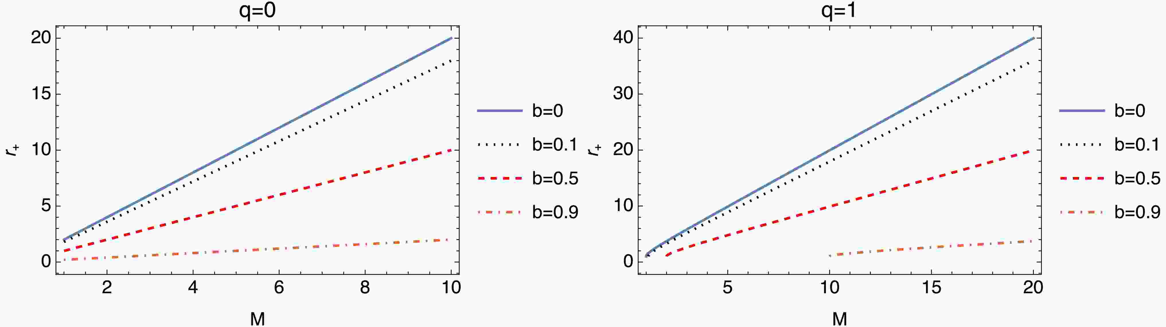
When $q \to 0$, these results align with those of previous studies [68−68]. Figure 1 and Fig. 2 illustrate the behaviors of the horizons under different parameters and values. The plots of both figures demonstrate how the Lorentz-violating parameter b and charge q affect the horizon formation of the CBHwKRF. Higher values of b reduce the horizon radius showing that Lorentz violation plays a crucial role in determining the horizons.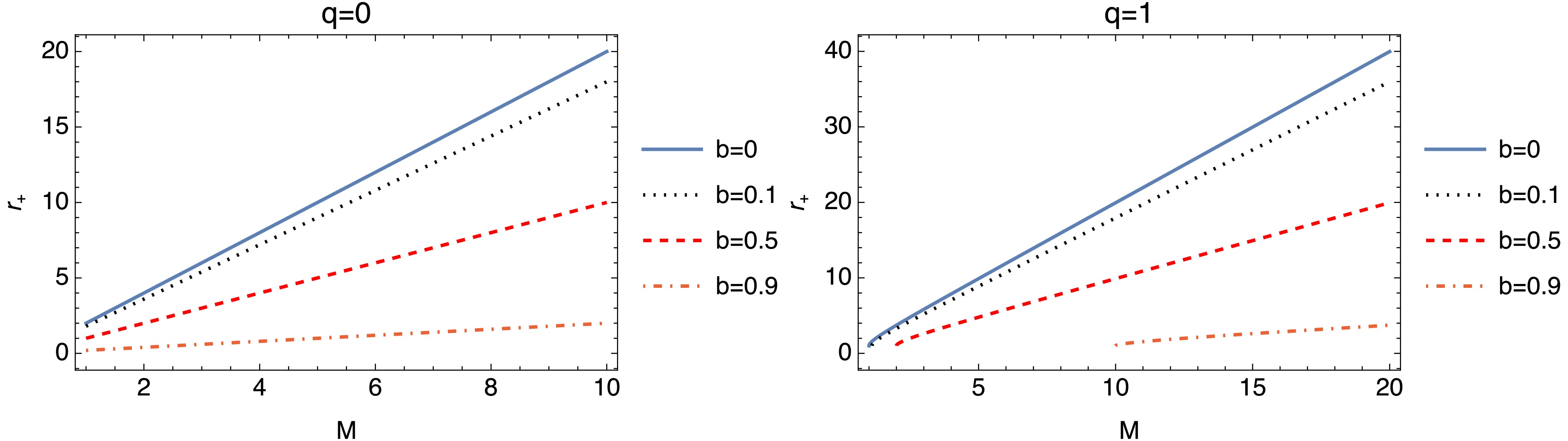

Figure 1.  (color online) Event horizon ($ r_+ $) versus mass graph. The plots are governed by Eq. (5).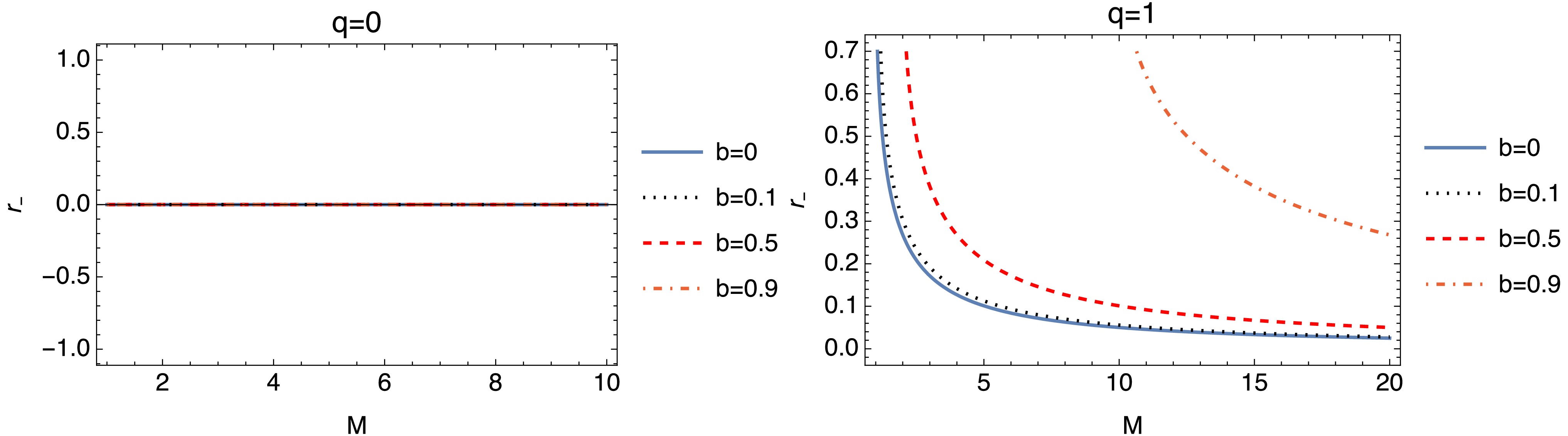

Figure 2.  (color online) Inner or Cauchy horizon ($ r_- $) versus mass graph. The plots are governed by Eq. (5).

The following exact differential form can define the thermodynamic structure of the thermal system, which is the so-called first law of thermodynamics of black holes [68, 69]:

where $ T_{H} $ is the black-hole or Hawking temperature, S is the black hole or so-called Hawking-Bekenstein entropy, and Φ is the electric potential given in Eq. (7). If we substitute $ r=r_{+} $ into the metric function, the metric function tends to zero, and the mass of the black hole can be calculated as follows:

In geometric units ($ G=c=\hbar=1 $), the Hawking-Bekenstein entropy for standard spherically symmetric black holes is given by [70]

Therefore, one can rewrite Eq. (7) as follows:

Now we can use the Euler homogeneous-function theorem to determine the Smarr formula [71]. Based on Euler's homogeneous theorem, the two-variable homogeneous function of order n is given by

where λ is a constant and $ (i,j,k) $ are integer powers [72]. For this case, the differentiation of Eq. (10) becomes

When we choose $(i=2n,\, j=n)$ and define the new shifted variables as $(S \rightarrow \lambda^{i} S,\; q \rightarrow \lambda^{j} q)$, the Smarr formula is constructed as follows using Eq. (9) and Eq. (10):

To find the Hawking temperature, $ T_{H} $ can be isolated from Eq. (6):

which results in

or

However, the result can be checked by considering the surface gravity κ, which is calculated from the derivative of the metric function at the event horizon [73]:

where a prime symbol denotes the derivative with respect to r. Evaluating this at $ r = r_{+} $, we have

Substituting the expression for M:

we obtain

The surface gravity (ξ) of a spherically symmetric static metric is given by [73]

Thus,

Because the Hawking temperature ($ T_H $) [73] is defined by

we can obtain

which is in good agreement with the result obtained in Eq. (15).

The subsequent derivative in the Smarr formula specifies the electric potential energy at the horizon. Therefore, the electric-potential interaction is represented by

In addition, the electric field of CBHwKRF spacetime is given by

In summary, the compact Smarr expression can be written as follows:

Moreover, we can calculate the heat capacity [74, 75], which plays a key role in the analysis of thermal stability, using the following formula:

Thus, the heat capacity may be determined as follows:

The plots presented in Fig. 3 illustrate the behavior of the quantity $ C_H $ as a function of r, under different settings of the parameters q and b. Each subplot corresponds to a unique value of q, showing the variation in $ C_H $ with $ r_+ $ for different values of b. For $ q = 0 $, the system remains thermally stable with no divergences. As q increases, divergences emerge (becoming more pronounced at higher q) while an increasing b mitigates these effects by smoothing the transitions and shifting critical points to a larger $ r_+ $. This suggests that b plays a stabilizing role in the thermodynamic behavior of the system.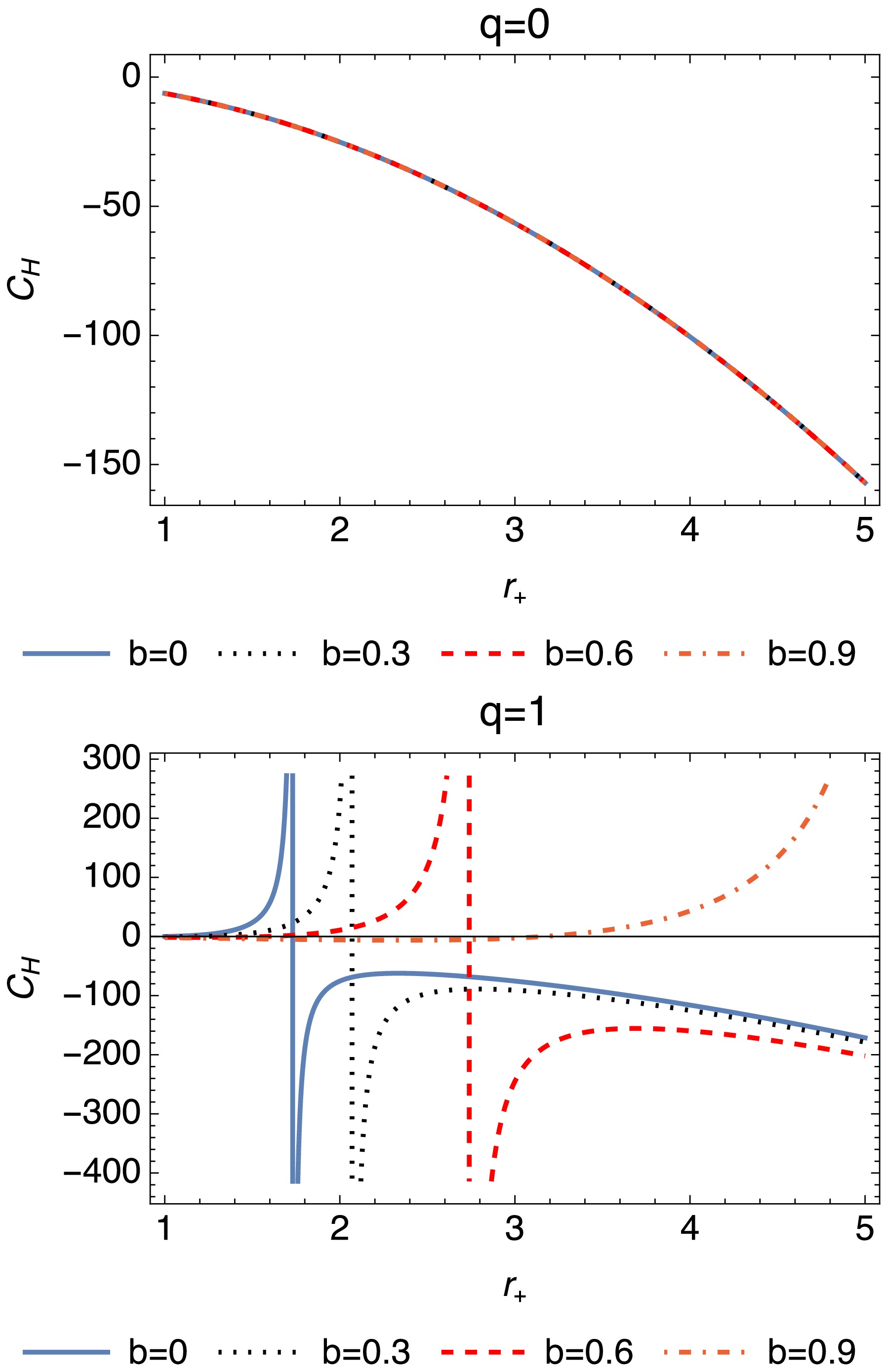

Figure 3.  (color online) Plots of $ C_{H} $ are governed by Eq. (27).

Our analysis focuses on the outer spacetime of the black hole, relevant for astrophysical observations. For $ q > q_{\text{crit}} = \sqrt{(1-b)^3}M $, a naked singularity forms; however, we restrict our study to regimes where the outer horizon exists, enabling the examination of thermodynamic and lensing properties. The thermodynamic behavior of a charged black hole with Lorentz-symmetry violation shows critical phenomena in $ C_H $, signaling second-order phase transitions. However, the Helmholtz free energy F [76] does not exhibit similar transitions, likely due to the influence of b. This suggests a modified thermodynamic framework, where conventional phase-transition behavior may not apply. The existence of critical points in $ C_H $ underscores the system complexity, warranting future investigation for deeper insights.

Standard thermodynamic analysis, supplemented by corrections from statistical mechanics, allows us to examine thermal fluctuations in the structures considered [77, 78]. These corrections lead to notable variations in the classical thermodynamic potentials. In this context, if the system is in thermal equilibrium, the density of states is given by [79]

where $ S_0 $ represents the uncorrected entropy, and $ \beta_0=1/T_H $. The formula for the logarithmic corrected (LC) entropy is given as

where $ S_{0}=\pi r^{2}_{+} $ and α is the parameter representing thermal fluctuations [79]. Notably, $ \alpha=1 $ corresponds to the maximum effect of thermal fluctuations [79, 80]. Substituting Eq. (15) and Eq. (28) into Eq. (30), the LC entropy of the CBHwKRF spacetime can be expressed as

The plots provided in Fig. 4 illustrate the behavior of the quantity $ S^{LC} $ as a function of the event horizon $ r_+ $ for various settings of the parameters q and b. Each plot is indicative of how $ S^{LC} $ responds to changes in $ r_+ $ under different parameter configurations. As q increases, the behavior of $ S^{LC} $ transitions from linear and predictable (for $ q = 0 $) to complex and non-linear (for $ q = 1.5 $). Higher q values introduce intricate interactions and abrupt changes, highlighting the sensitivity of the system entropy to both $ r_+ $ and b. This suggests a critical role for q in driving the thermodynamic complexity of the black hole. With this new expression for entropy, we can analyze significant thermodynamic energies and expressions under the influence of maximum thermal fluctuations $ (\alpha=1) $. First, let us calculate the internal energy formulated as

Figure 4.  (color online) Plots of $ S^{LC} $ are governed by Eq. (31) under the influence of maximum thermal fluctuations $ (\alpha=1) $.

Upon substituting $ (T_H) $ and the differential of $ (S^{LC}) $ into Eq. (32) and integrating, the internal energy is determined as follows:

The graphs of Fig. 5 illustrate the variation of a physical quantity, $ E^{LC} $, with respect to the event-horizon radius $ r_+ $for different values of the charge parameter q and parameter b. As q increases, the behavior of $ E^{LC} $ shifts from linear and stable (for $ q = 0 $) to non-linear and complex (for $ q = 1.5 $). Higher q values highlight intricate interactions and a stronger influence of b, especially as $ E^{LC} $ transitions to non-monotonic or decreasing trends with $ r_+ $.

Figure 5.  (color online) Plots of $ E^{LC} $ are governed by Eq. (33).

The expression for the corrected Helmholtz free energy $ (F^{LC}) $ is given by

Integrating Eqs. (15) and (31) into Eq. (34), the corrected Helmholtz free energy can be formulated as

The plots of Fig. 6 represent the variation of the quantity $ F^{LC} $ with respect to the radius of the event horizon r, for different values of the parameters q and b. For $ q = 0 $, $ F^{LC} $ exhibits a linear increase with $ r_+ $, maintaining a stable dependence on b. As q increases, particularly at $ q = 1.5 $, this growth slows, with higher b values causing a plateau or slight decline. Overall, increasing b mitigates these fluctuations, underscoring its crucial role in governing the thermodynamic behavior of the system.

Figure 6.  (color online) Plots of $ F^{LC} $ are governed by Eq. (35).

Referring to the definition of Helmholtz free energy $ (F=E-TS) $, the pressure of the black hole is expressed as

where $ V=\dfrac{4}{3}\pi r^{3}_{H} $, represents the volume of the black hole. Substituting Eq. (35) into Eq. (36) and deriving the expression for pressure, we obtain

The plots given in Fig. 7 illustrate the behavior of the physical quantity $ P_{LC} $ as a function of the event-horizon radius $ r_+$, parameterized by charge q and another variable b. For $ q=0 $, $ P_{LC} $ decreases monotonically with $ r_+ $, stabilizing as it approaches zero. As q increases, a peak emerges for certain b values, followed by a decline, indicating more complex interactions. For example, at $ q=1.5 $, the behavior becomes increasingly varied, with $ P_{LC} $ crossing zero or exhibiting chaotic fluctuations, highlighting significant dependencies on both b and $ r_+ $. Overall, these trends reveal intricate dynamics influenced by the parameters q and b.

Figure 7.  (color online) Plots of $ P^{LC} $ are governed by Eq. (37).

Furthermore, the enthalpy $ (H) $ is defined as follows:

By substituting the corresponding values of internal energy, pressure, and volume into Eq. (38), we derive

As illustrated in Fig. 8, for $ q=0 $, $ H_{LC} $ displays a linear relationship with $ r_+ $, consistent across all b values. With increasing q, such as $ q=1.5 $, linearity continues, but with minor slope differences influenced by b, where higher b values result in a more gradual rise. These variations do not disrupt the primary proportionality between $ H_{LC} $ and $ r_+ $, as b mainly modulates the growth rate without altering the fundamental trend.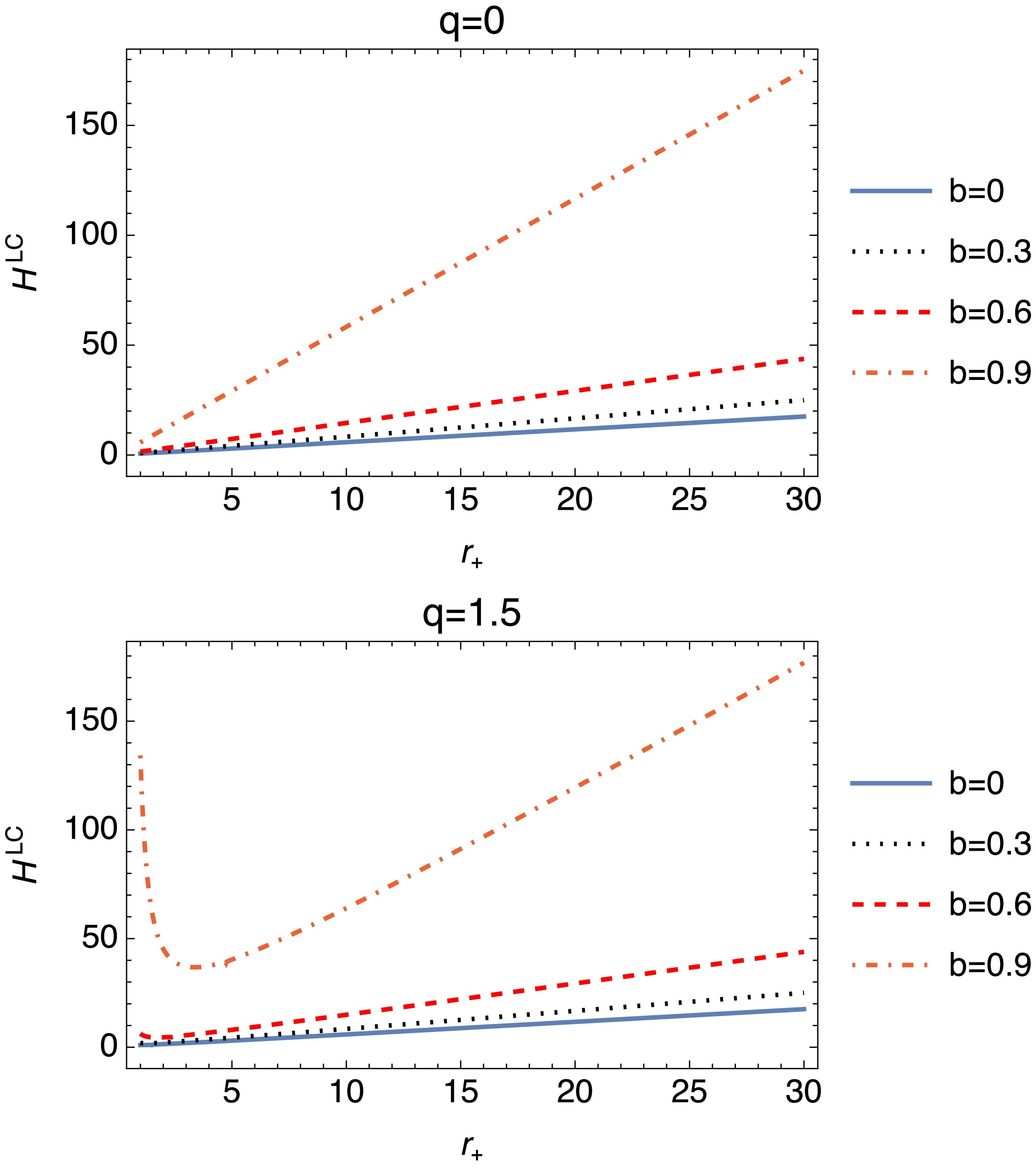

Figure 8.  (color online) Plots of $ H^{LC} $ are governed by Eq. (39).

The thermodynamic expression for the Gibbs free energy $ (G) $ can be written as follows:

When the values of $ F^{LC} $, $ P^{LC} $, and V are substituted into Eq. (40), the Gibbs free energy reduces to

The plots of $ G_{LC} $ in Fig. 9 show a consistent increase with $ r_+ $ across all q values, with $ q = 0 $ starting at a lower value and exhibiting a steeper slope compared to higher q values, such as $ q=2 $. As b increases, the initial value of $ G_{LC} $ at $ r_+ = 5 $ decreases, while the growth rate remains largely unaffected, indicating that b primarily shifts the baseline without altering the trend. Overall, $ G_{LC} $ demonstrates a strong dependence on $ r_+ $, with b modulating its initial value across different charge scenarios.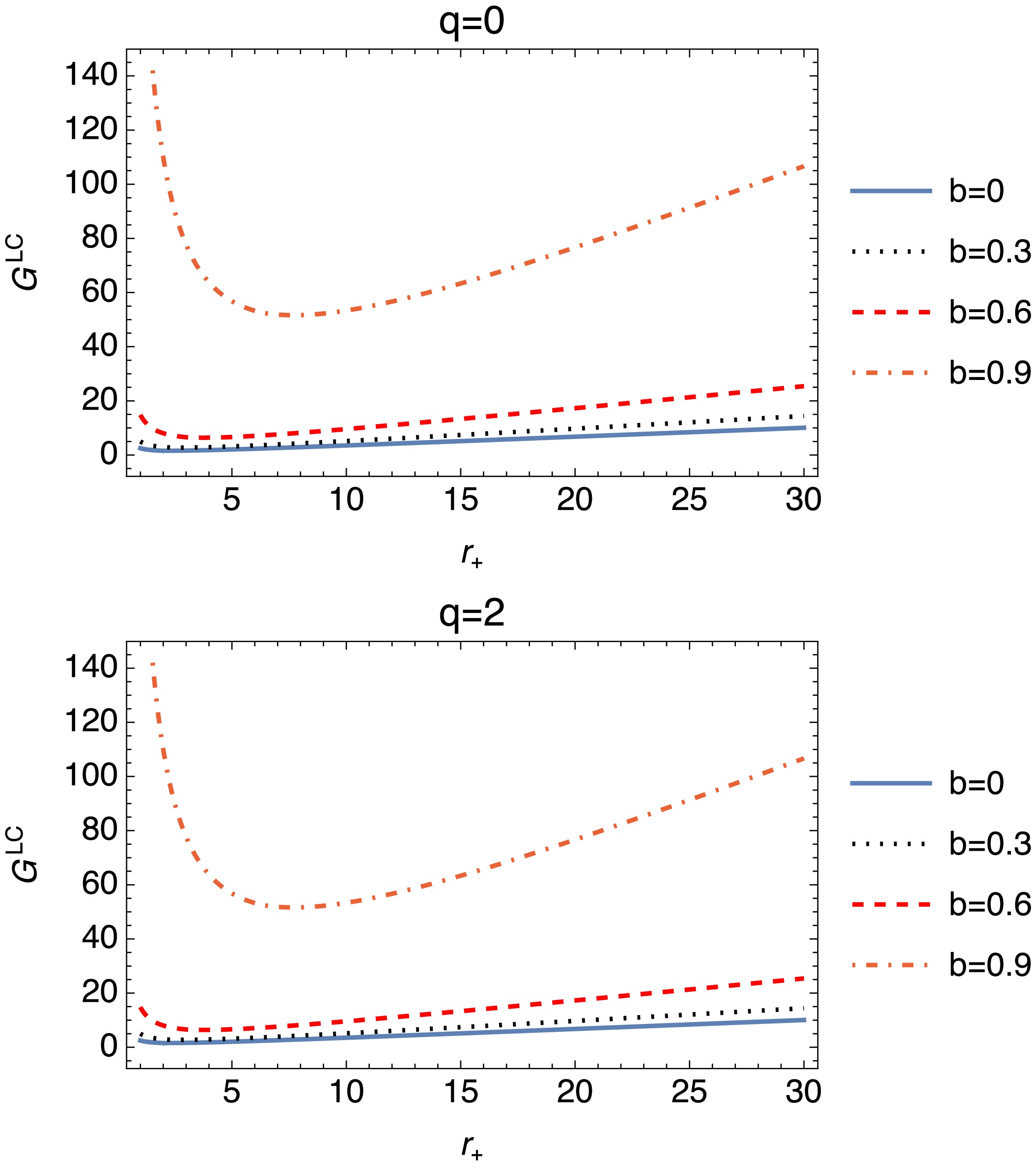

Figure 9.  (color online) Plots of $ G^{LC} $ are governed by Eq. (41).

The corrected specific heat $ (C^{LC}) $ can be described as follows:

Using Eq. (33) and Eq. (15), we can compute the expression governing the corrected specific heat of black holes. Consequently, the corrected specific heat is expressed as

The plots in Fig. 10 show that for $ q=0 $, $ C^{LC} $ decreases smoothly with increasing $ r_+ $, indicating predictable thermal behavior. At higher q values (i.e., $ q=2 $), the behavior becomes more complex, with fluctuations and divergences near specific $ r_+ $ values. An increasing b value stabilizes these fluctuations, moderating the abrupt changes and shifting critical points to a higher $ r_+ $, thereby highlighting its role in improving the thermal stability of the system. Moreover, Fig. 10 highlights the sensitivity of $ C_{LC} $ to the thermal-fluctuation parameter α alongside q and b. For $ q=2 $, higher b values shift the divergence point of $ C_{LC} $ to larger $ r_+ $, indicating that the instability occurs in larger black holes. This emphasizes the role of b in modulating thermal properties and stability.

Figure 10.  (color online) Plots of $ C^{LC} $ are governed by Eq. (43).

The isothermal compressibility, which plays an important role in stability, is defined as

Notably, the condition $ \kappa\geq 0 $ ensures that the system returns to equilibrium under spontaneous changes of the parameters, and this is known as Le Chatelier's principle [81]. By substituting Eq. (37) into Eq. (44) and using the chain rule, the isothermal compressibility can be written as

Figure 11 illustrates the behavior of the isothermal compressibility κ as a function of $ r_+ $. For $ q = 0 $, κ remains positive and increases with $ r_+ $ across all b values, indicating stable thermodynamic behavior. In contrast, for higher q values such as $ q = 1.5 $, κ exhibits regions of negativity, particularly for higher b values, signaling instability in certain parameter ranges. Additionally, divergence points appear, highlighting regions of extreme compressibility. This suggests that both q and b play crucial roles in determining stability, with higher values leading to greater instability.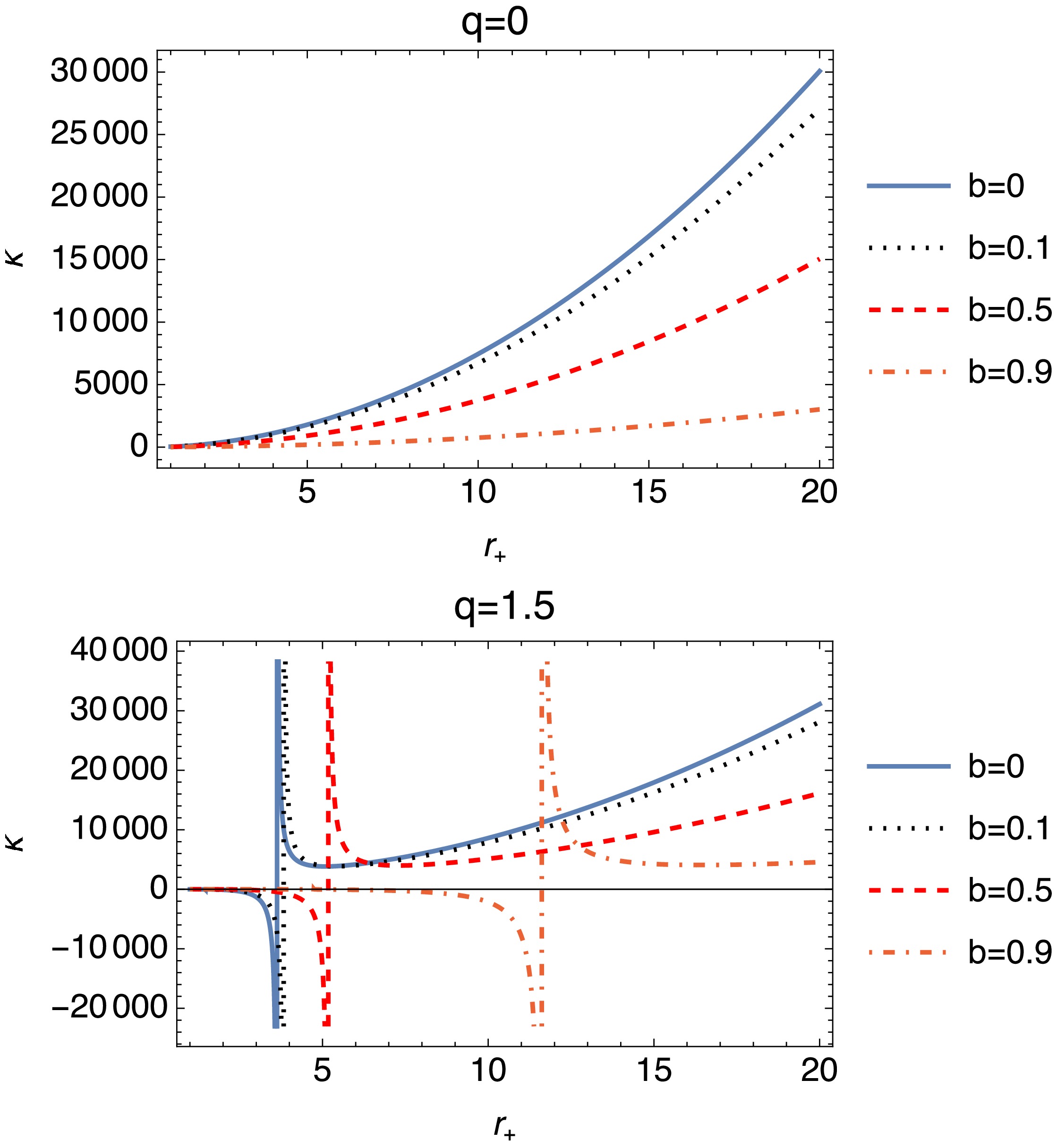

Figure 11.  (color online) Plots of the isothermal compressibility with respect to the event horizon. The graphs are governed by Eq. (44).

In summary, our thermodynamic analysis notably advances LSV studies, particularly concerning charged black holes in KR-field models. Unlike previous studies that predominantly explore uncharged black holes or simplified LSV contexts, our study investigates the relationship between the LSV parameter b and charge Q, revealing unique fluctuation behaviors in thermodynamic quantities such as the Hawking temperature T, heat capacity $ C_P $, and Helmholtz free energy F. The critical transitions observed in $ C_P $ demonstrate a distinct dependence on b, setting our findings apart from other modified-gravity scenarios. Additionally, our work integrates gravitational-lensing effects using the Gauss-Bonnet theorem to establish an observational link to LSV. The explicit deflection-angle calculations provide insights into the astrophysical manifestations of the KR field, offering a complementary perspective to the thermodynamic results. This dual approach—bridging black-hole thermodynamics and astrophysical observables—enhances the significance of our analysis. Thus, our study contributes to the literature by extending LSV effects to charged black holes in KR-field models, uncovering novel thermodynamic characteristics, and providing an observational context through lensing analysis.

One of the renowned predictions of Einstein's theory of relativity is the gravitational-lensing effect, which provides an experimental verification of the theory. Rindler and Ishak (RI) investigated a lensing-analysis method using the generalization of the inner product in a Riemannian manifold [82]. In the symmetry plane ($ \theta=\pi/2 $), the generic RI lensing-geometry structure can be illustrated as follows:

The lensing invariant between the path of light (d) and radial line (δ), as shown in Fig. 1, is given by

where $ g_{ij} $ is the metric tensor of the spacetime. The geometrical coordinates of the lensing geometry are defined by

where $A(r,\varphi) \equiv \dfrac{{\rm d}r}{{\rm d}\varphi}.$ When the information from Eq. (47) is substituted into Eq. (46), the invariant formula simplifies to

Consequently, the one-sided bending angle can be measured as $ \epsilon = \psi - \varphi $. Moreover, we can calculate the light trajectory by solving the null geodesics equation. In this context, the RI lensing-geometry line-element (optical metric) for standard spherically symmetric spacetimes at a constant time slice can be written as follows:

where $ f(r) $ is the metric function of the given spacetime. If E and L represent energy and angular momentum, respectively, the constraints of the null geodesics equations are given by

Here, τ is the proper time. Combining the constraints, the general null geodesics equation becomes

Defining the new variable $ u = \dfrac{1}{r} $ ($ u \ll 1 $), the second-order differential form of Eq. (51) is

Substituting the metric function into Eq. (52), the null geodesics equation for the spacetime reads

where $ \beta = 1/(1-b) $. Equation (53) represents a second-order nonlinear differential equation; however, we can solve the equation using a well-known perturbative solution method. In this method, we consider the solution of the linear and homogeneous differential equation, $\dfrac{{\rm d}^{2}u}{{\rm d}\varphi^{2}} + \beta u = 0$, in the form of $ u(\varphi) = \dfrac{\sin(\sqrt{\beta} \varphi)}{R} $. Note that R is called the impact parameter and $ R \gg 1 $. When we substitute the solution of the linear and homogeneous differential equation into the nonlinear part of Eq. (53), the perturbative solution of Eq. (53) is given by

Moreover, the derivative of $ u(\varphi) $ with respect to φ is

If we choose $ \theta=\pi/2 $ in Eq. (54), the parameter representing the minimum distance between a light ray and massive object during gravitational lensing $ r_0 $, known as the closest approach distance, is determined to be

When we set $ \varphi = 0 $ and consider $ R \gg 1 $, the dominant terms of Eq. (54) and Eq. (55) are as follows:

Based on the information in Eq. (57), Eq. (48) can be rewritten as

The parameter b, and hence β, which characterizes the extent of the Lorentz-symmetry violation, can indeed have observable consequences in the context of gravitational lensing. Although current astrophysical observables are not finely tuned to detect such small deviations from general relativity, future high-precision measurements, especially in the vicinity of compact objects such as supermassive black holes or neutron stars, could provide a method to constrain b. For example, gravitational-lensing experiments, using techniques such as very long baseline interferometry (VLBI) [83] in the Event Horizon Telescope (EHT) [84], can detect minute deviations in the bending angle of light, which are sensitive to the Lorentz-violating effects encapsulated by b.

The influence of b on the lensing angle (Eq. (58)) suggests that larger deviations from zero would manifest as an enhancement of the lensing effect, particularly noticeable in regions of strong gravitational fields. This offers a potential pathway for using gravitational lensing as a probe for the Lorentz-symmetry violation in future astrophysical observations.

Astrophysics continually benefits from the theoretical frameworks provided by general relativity, particularly in understanding phenomena such as gravitational lensing and redshift. This section explores significant astrophysical applications that rely on the principles of general relativity to explain the behavior of compact stars. We present empirical data and theoretical analyses that not only validate these principles, but also help in estimating key celestial parameters. Additionally, the impact of Lorentz-violation parameters on these phenomena is examined, offering insights into their potential implications on the conventional understanding of spacetime dynamics.

As shown in Table 1, we list the mass, radius, and electric-charge values for three different charged compact stars [79]. These data provide insight into how varying masses and radii correlate with relatively large electric charges (on the order of $10^{20} $ C), which can influence gravitational lensing and redshift effects. In the graphical analysis, we used standard international units (S.I units) with conversion factors $G \mathrm {c^{-2}}$ and $G^{1/2}{\mathrm c^{-2}}(4\pi \varepsilon _{0})^{-1/2}$ for mass and charge, respectively. Note that, $G= 6.67408\times 10^{-11}\;{\rm m}^{3}{\rm{kg}}^{-1}{\rm s}^{-2}$, $ c=3\times 10^{8}\;{\rm{ms}}^{-1} $, and $\varepsilon _{0}=8.85418\times 10^{-12}\;{\rm C}^{2}{\rm N}^{-1}{\rm m}^{2}$.

Charged Compact Stars	Mass $/M_{\odot}$	Radius /km	Electric Charge /C
Vela X-1	$ 1.77M_{\odot} $	$ 9.56 $	$ 1.81\times 10^{20} $
SAXJ 1808.4-3658	$ 1.435M_{\odot} $	$ 7.07 $	$ 1.87\times 10^{20} $
4U 1820-30	$ 2.25M_{\odot} $	$ 10 $	$ 1.89\times 10^{20} $

Table 1.  Tabulated numerical values of mass, radius, and electric charge for compact stars expressed in solar masses ($ M_{\odot} $) [85].

In Fig. 12, the one-sided bending angles of the compact stars are plotted for the RN limit $ (b=0) $ and the maximum value of the horizon condition $(1-b= \left({M}/{q}\right)^{2/3})$. For all compact stars, the Lorentz-violation parameter b plays a crucial role as the lensing effect increases dramatically when b approaches $1-\left({M}/{q}\right)^{2/3}$.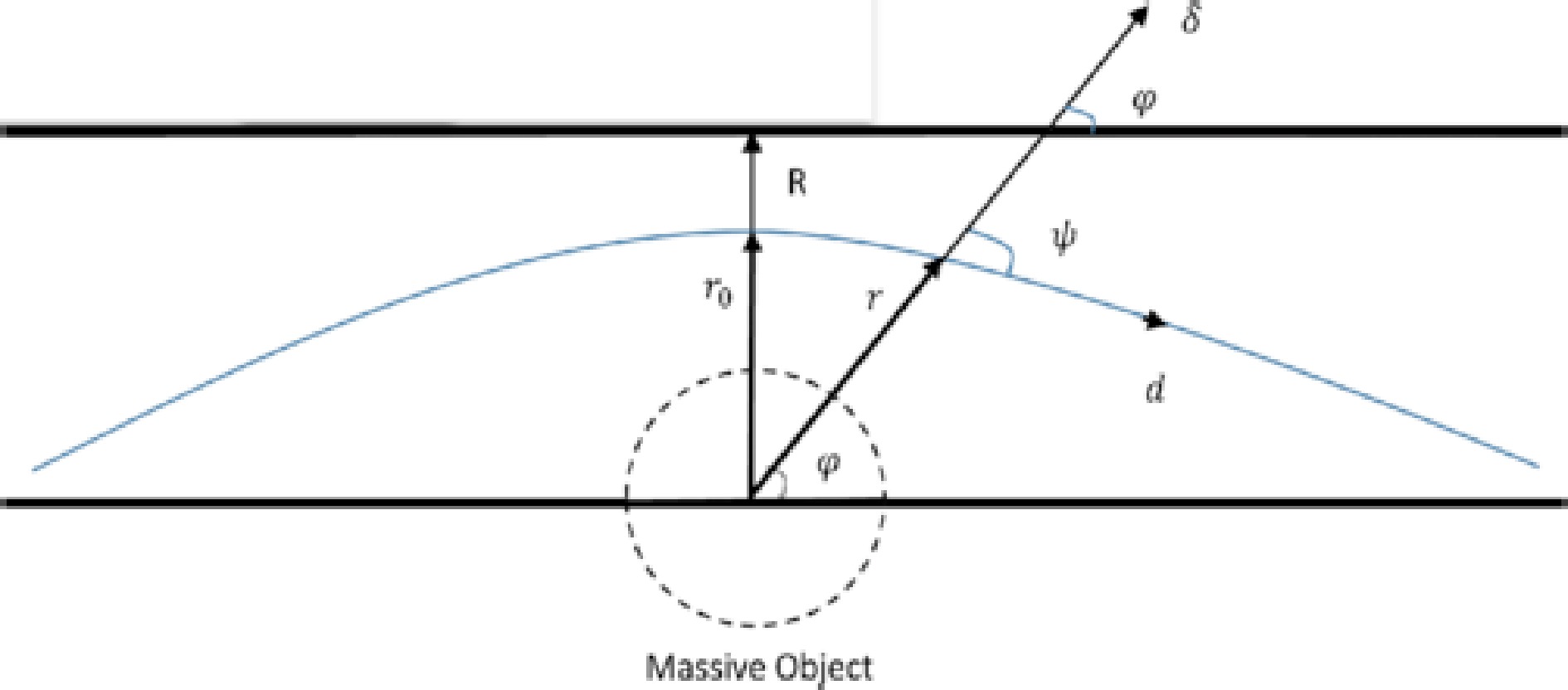

Figure 12.  (color online) General bending of light geometry of the RI method

Another intriguing astronomical effect from Einstein's theory of general relativity is gravitational redshift. For static spacetimes, the gravitational redshift is given by

where $ \lambda_O $ and $ \lambda_e $ are the observed and emitted wavelengths, respectively [86, 87]. Substituting $ f(r) $ into Eq. (59) under the assumption of large r ($ r \rightarrow R $ and $ R>>1 $), Eq. (59) simplifies to

In Fig. 13, we observe a similar graphical structure for gravitational-redshift values of compact objects as in the bending of light analysis. In these graphs, the Lorentz violation contributes positively. Figure 14 compares the gravitational-redshift parameter $z $ for both the RN limit (b = 0) and Lorentz-violating case $(1-b=\left({M}/{q}\right)^{2/3})$ as a function of R/R_star. In each subplot, the presence of the Lorentz-symmetry violation enhances the redshift at smaller radii, indicating a stronger gravitational effect. As R/R_star increases, the two curves gradually converge, revealing that the Lorentz-violating effects diminish at larger distances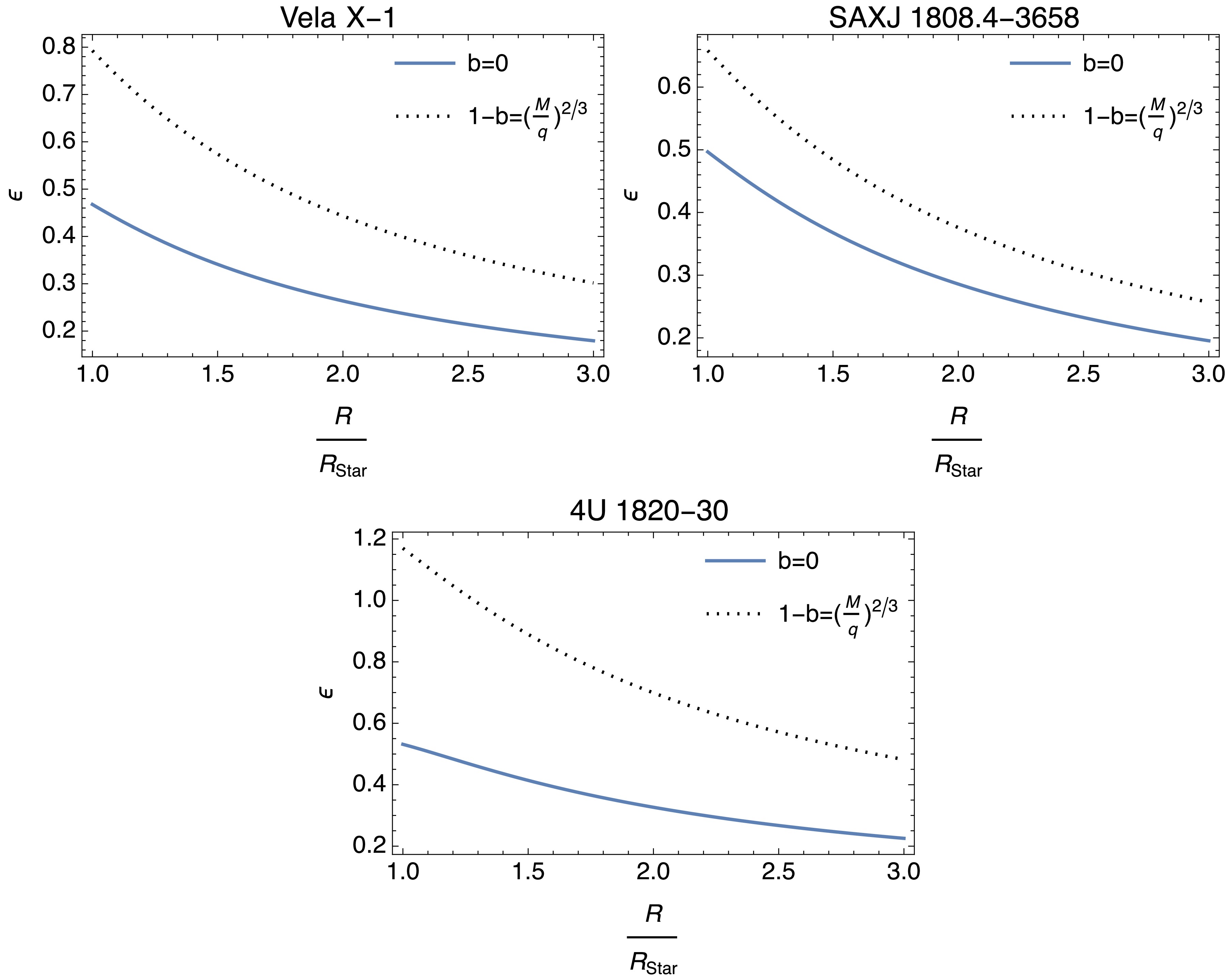

Figure 13.  (color online) These figures depict how the bending angle $ \epsilon $ changes with respect to $ R/R_{\text{star}} $ for charged compact stars. Each graph compares the RN case ($ b=0 $) with the Lorentz-violation effect ($ b\neq0 $).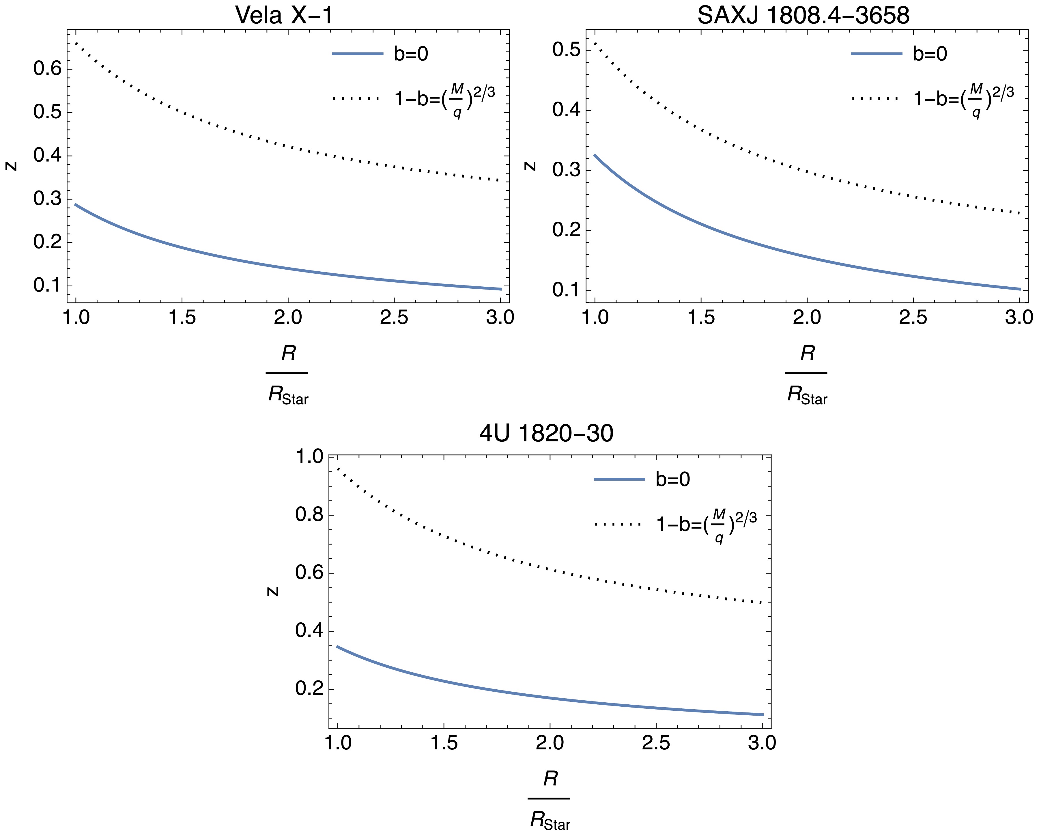

Figure 14.  (color online) These graphs show how the gravitational-redshift parameter z evolves with respect to $ R/R_{\text{star}} $ for compact objects. Each graph includes trends for both the RN limit ($ b=0 $) and Lorentz-violation effect ($ b\neq0 $).

Finally, we aim to analyze potential constraints on b related to thermal attributes and lensing observations. Given the influence of b on black-hole thermodynamics and lensing, constraints are derived from criticality conditions in these areas. Typically, the thermodynamic-stability criteria are used to derive the thermal-threshold parameter $ b_{\text{crit,thermal}} $ on b. For a CBHwKRF, this condition is linked to the behavior of the heat capacity $ C_H $, which undergoes divergence at a phase transition. The critical value of b is determined by solving the condition for the divergence:

The divergence occurs when $ \dfrac{\partial T}{\partial r_{+}}=0 $. Differentiating $ T_H $ with respect to $ r_+ $, we obtain

Setting Eq. (62) to zero, we obtain the following condition:

Solving for $ b_{\text{crit,thermal}} $ gives

The photon-sphere condition [88−90] is provided as follows:

in which a prime symbol denotes the derivative with respect to r. Substituting Eq. (4), $f(r, b)\equiv A(r)$, into Eq. (65), we have

After solving for $ b_{\text{crit,lensing}} $, we obtain

These derivations explicitly highlight the dependencies of the critical values of b on the black-hole parameters q, $ r_+ $, M, and $ r_{\text{ph}} $. They also demonstrate how b plays a pivotal role in both thermodynamic and optical behavior. The explicit constraints on b bridge the thermodynamic and lensing phenomena in CBHwKRF spacetimes. These results may provide a direct method to link theoretical predictions with future astrophysical observations, enabling a more comprehensive analysis of Lorentz violation in the context of charged black holes.

This study has systematically explored the influence of Lorentz-symmetry violation on the gravitational lensing and thermodynamic properties of CBHwKRF. The findings have revealed marked modifications in both gravitational and thermodynamic behaviors resulting from Lorentz-symmetry violation, elucidated through a detailed analysis of the space-time metrics and their astrophysical implications.

The gravitational-lensing analysis, employing the RI method modified for Lorentz-violating spacetimes, indicated that the Lorentz-violating parameters notably enhance the bending angles of light around black holes. This enhancement, as shown in the graphical representations of Fig. 13, underscores the potential for observing such deviations in environments harboring compact objects. The bending angles were sensitive to variations in the Lorentz-violating parameter b (or $ \beta=1/(1-b) $), as quantified by Eq. (58), suggesting observable effects in real-world astrophysical scenarios.

Thermodynamically, the inclusion of the KR field introduced significant changes in the Hawking temperature, entropy, and specific heat of the black holes. The first law of thermodynamics, represented in Eq. (6), and the Smarr formula in Eq. (26) emphasize the non-trivial contributions of the Lorentz-violating terms to black-hole thermodynamics. In particular, the graphical analyses in Figs. 3−10 elucidate the impact of Lorentz violation on thermodynamics across different configurations of the CBHwKRF. The introduction of LC thermal fluctuations has further refined our understanding of the modified entropy, energy, enthalpy, and specific-heat profiles, illustrating the extended implications of quantum-gravity corrections under Lorentz-symmetry breaking.

The relationship between thermodynamic properties and gravitational-lensing phenomena becomes particularly intriguing within the framework of LSV theories. In our study, the KR-field parameter b serves as a crucial link influencing both the thermodynamic behavior and deflection of light. Thermodynamic quantities such as the Hawking temperature T and entropy S depend explicitly on the metric function, which governs the spacetime geometry around the black hole. Similarly, gravitational lensing, characterized by the deflection angle α, is sensitive to the same geometric structure, particularly to the effects introduced by b. Recent studies such as [91] highlight how critical thermodynamic points, such as phase transitions marked by heat capacity $ C_P $, correlate with changes in the deflection angle α. In our analysis, the KR-field parameter b modifies the metric function in a way that simultaneously impacts the photon sphere and thermodynamic stability. This shared dependence on the metric establishes an indirect but profound connection between the two phenomena, providing a novel perspective within the LSV framework. This relationship between thermodynamics and gravitational lensing not only enhances our understanding of black-hole physics, but also offers potential observational probes for testing the validity of LSV models. By combining thermodynamic and lensing analyses, a unified framework emerges to explore the broader implications of LSV theories.

In conclusion, our study provides a comprehensive investigation of the effects of Lorentz-symmetry violation on gravitational lensing and black-hole thermodynamics in the presence of the KR field. Future work should focus on the observational validation of these theoretical predictions, particularly through high-precision astrophysical measurements [92]. Such investigations may profoundly impact our understanding of fundamental physics, offering new insights into the nature of Lorentz-symmetry violations and their observable signatures in cosmological phenomena. Moreover, extending this analysis to include rotating (and/or higher dimensional) black holes and examining interactions with nearby astrophysical objects can uncover further nuances in the relationship between Lorentz-violating fields and gravitational dynamics.

We acknowledge the networking support of COST Actions CA21106, CA22113, and CA23130. We also thank EMU, TÜBİTAK, SCOAP³, and ANKOS for their support.