


 Abstract
 HTML
HTML Reference
 Related
 PDF
PDF


-
The Wide Field of view (FOV) Cherenkov/Fluorescence Telescope Array (WFCTA) is a major component of the Large High Altitude Air Shower Observatory (LHAASO) [1]. The main features of these third generation telescopes are: i) small silicon photomultiplier (SiPM) pixels on the camera with a
$ 0.5^{\circ} $ FOV; ii) precise electronics with 50 MHz flash analog-to-digital converter (FADC); and iii) optimized optics [2]. The main goals of the WFCTA are to measure the cosmic ray (CR) energy spectrum and composition accurately from 100 TeV to several EeV. Because the CRs observed by the WFCTA cover a wide energy range of over four orders of magnitude, two detection techniques are adopted, using the same telescopes with different detector configurations. Below 100 PeV, the Cherenkov technique is used. It is divided into two phases with energies from 100 TeV to 10 PeV [3] and 10 to 100 PeV [4], respectively. Above 100 PeV, the fluorescent light observation mode is utilized. This paper describes the geometrical reconstruction of extensive air showers (EASs) viewed by the WFCTA in the fluorescent light observation mode.In fluorescent light observation mode, the WFCTA experiment is composed of 20 telescopes distributed over three sites to form a stereo-viewing system. When an EAS propagates through the FOV of the telescope array, its track will be recorded by at least two sites simultaneously. To obtain all the primary EAS information, such as the energy and
$ X_{\max} $ , which will be used in the CR energy spectrum measurement and composition discrimination, one has to consider the propagation of the EAS along its track. Thus an accurate determination of the EAS trajectory is vital. The trajectory can be reconstructed by one or two sites (mono or stereo reconstruction, respectively). Mono reconstruction uses the triggering time of the SiPMs to determine the orientation of the EAS, while stereo reconstruction uses the intersection of two shower-detector-planes (SDPs) determined by the shower track and the detectors. The results of experiments such as HiRes and Auger indicate that stereo reconstruction (using only geometrical information from two 'eyes') is superior to mono reconstruction (using geometrical and timing information from one 'eye') [5, 6]. Two different methods of stereo reconstruction for the tracks observed by the WFCTA have been investigated. In the reconstruction, the key issue is to obtain the SDPs. In the first method, only the geometrical information of the triggered SiPMs is used, while in the second one, to fully exploit the high-speed electronics, the triggering time is also used [5, 6].In this study, these two methods are investigated in detail through WFCTA simulated fluorescence events. The paper is structured as follows. First, a description of the WFCTA experiment in fluorescent light observation mode is provided. Two geometrical reconstruction approaches are then introduced, followed by a discussion of reconstructed resolution. Finally, conclusions are presented.
-
The WFCTA is composed of 20 telescopes in fluorescent light observation mode. As shown in Fig. 1, the telescopes are located at the three vertices of an isosceles triangle with a base line of 10 km and a height of 5 km. The telescope arrays at the three vertices are named FD1, FD2 and FD3, respectively. At FD1, 16 telescopes are configured as a
$ 4\times4 $ array, covering a range of$ 64^{\circ} $ in azimuth and$ 64^{\circ} $ in elevation starting from$ 3^{\circ} $ . The FD2 and FD3 sites, having 2 telescopes each, are located at the bottom vertices. They are configured as a$ 1\times2 $ array, covering a range of$ 32^{\circ} $ in azimuth and$ 16^{\circ} $ in elevation starting from$ 3^{\circ} $ .
Figure 1. (color online) Configuration of WFCTA in fluorescence mode. The small solid circles represent fluorescence telescopes; the arrows illustrate the detector FOV along the azimuth; the large circle close to the center of the FOV represents the ground array of LHAASO. Their relative locations in the coordinate system are displayed at the bottom right.
Each telescope has a spherical reflector made of 20 full and 5 half hexagonal mirror segments. A ray tracing procedure, considering the shadowing of the camera and the gaps between the mirror segments, indicates that the geometrical effective area of the mirror is approximately
$ 4.7 {\rm m}^{2} $ . The imaging camera is constituted of 1024 SiPMs, forming a$ 32\times 32 $ array with a FOV of$ 16^{\circ} \times 16^{\circ} $ . Each SiPM in the camera is a square with a side length of 15.0 mm [2]. A Winston-cone, with the upper and lower square surfaces of 25.4 and 15.0 mm in length, respectively, and with an angular aperture of$ 0.5^{\circ} $ , is coupled to each SiPM. Each SiPM is read out by a 50 MHz FADC to measure the shower signals, with a typical duration of 20 ns. A peak finding algorithm has been developed in order to provide an individual SiPM trigger using a field programmable gate array (FPGA).Three trigger levels are required for event detection. The first is set by requiring a signal-noise ratio greater than
$ 4.0\sigma $ for the FD1 telescopes and$ 3.5\sigma $ for the FD2 (or FD3) telescopes, where$ \sigma $ is a standard deviation describing the background fluctuation within a running window of 320 ns [7]. According to the simulations, there are two main types of pattern for the images of air showers detected by the WFCTA telescopes. Fluorescent light images of air showers seen from several kilometers away tend to make line-shaped patterns on the camera, whereas Cherenkov light images of showers hitting the telescope head-on tend to form round-shaped patterns. Therefore, pattern recognition is performed on patches of$ 6\times6 $ SiPMs running over the whole camera. The 'track-type' pattern requires at least six triggered pixels forming a straight line and the 'circular-type' pattern forms with a triggered SiPM surrounded by another six adjacent SiPMs. Details of the pattern recognition are given in Ref. [7]. It should be noted that the method described in this article does not attempt to reconstruct such Cherenkov events from the EAS shower. A second level trigger decision is based on which of the telescopes in the array has issued a trigger, and is therefore referred to as the telescope trigger. The third level of trigger requires that FD1 is triggered in coincidence with at least one other of the two FDs. -
A complete Monte Carlo simulation was carried out, beginning with EAS generation using CORSIKA (version 75600) [8]. The QGSJET-II-04 and Gheisha models were selected for the high and low energy interactions of particles, respectively. The zenith angle was set in the range of
$ 30^{\circ} $ to$ 60^{\circ} $ and the azimuth was from$ -180^{\circ} $ to$ 180^{\circ} $ . The energies were fixed at 100, 200, 300, 500, 700, 900 and 1100 PeV. The statistics are shown in Table 1. Given the large number of particles in the EAS above 100 PeV, a thinning option was chosen, setting different thinning levels for each energy. For each event, the shower's longitudinal development was recorded in steps of$ 5\; {\rm{g/cm^2}} $ . The development curve of charged particles was input into the simulation procedure of the WFCTA fluorescence experiment. Each event was used five times, by sampling the shower core in a range of$ 15\; {\rm{km}} \times 12\; {\rm{km}} $ . Reference [9] provides further details of light generation and propagation, as well as the response of the detectors.Parameter Values E/PeV 100 200 300 500 700 900 1100 N 5000 4000 3000 2500 2500 2500 2500 Table 1. Statistics of the CORSIKA events produced for this work.
-
When an EAS moves through the atmosphere at the speed of light, it isotropically emits fluorescent light along the shower axis, which can be traced back to the arrival direction of the primary particle. A trajectory will be observed by the telescopes viewing this EAS. The correct determination of this trajectory is vital for measuring all the information of this shower. Propagation and attenuation of the light along the shower axis have to be taken into account, while reconstructing the other fundamental parameters of the shower, like energy,
$ X_{\max} $ , etc. In principle, determination of the EAS trajectory is straightforward. A series of triggered SiPMs in an event define a great circle on the celestial sphere. An SDP can be defined as the plane containing the detector and this circle, and the trajectory can be determined by either one or two sites (mono and stereo reconstruction, respectively). Mono reconstruction uses SiPM triggering times to determine the orientation of the shower axis within the SDP, while stereo reconstruction relies on the intersection of SDPs from two sites to obtain the shower trajectory. Stereo reconstruction is used in the WFCTA experiment, as it is known to perform better than mono reconstruction even when the timing information is added. The two approaches used for the determination of the SDPs, i.e. stereo-angular fitting based on the pointing direction of triggered SiPMs, and stereo-timing fitting using SiPM triggering time, will be described in detail in this section. -
A trajectory can be found within the coordinate system of triggering time versus viewing angle of the SiPM (time-elevation space) for each event. In the simulation, all photons collected by one SiPM form a complete waveform according to their arrival time. Based on the measurement, night sky background (NSB) photons with a flux of 10 photons per microsecond per square meter of the light collector are randomly added to the waveform. The electronic noise, with a mean of 1.2 FADC counts per 20 ns, is also added to every channel. A typical signal pulse detected by a SiPM is shown in Fig. 2. As shown in the top panel of Fig. 3, many isolated SiPMs which are not in the trajectory can be triggered by the night sky background and electronics noise and mimic the weak signal of fluorescence light. For a reliable trajectory reconstruction, the noisy SiPMs are removed in three steps:

Figure 2. Distribution of the signal pulse for a typical SiPM. The total FADC bins are 900 for each SiPM. Here, to display the signal area clearly, only 300 FADC bins around the signal area are shown.

Figure 3. (color online) Triggering time distribution as a function of viewing angle of SiPMs. The dots are SiPMs. The red curves are the results of conic fitting to the data. (top) The distribution of surviving channels after applying the SNR cut. (middle) The distribution after applying a further cut on the SiPM triggering time. (bottom) The distribution applying also the trajectory fitting cuts.
● SNR suppression of triggered SiPM: The SiPMs marked as noisy channels by the signal-noise ratio (SNR) described in Sec. II are removed.
● SiPM triggering time: Once a photon gets into a SiPM, its arrival time is recorded and referred to as
$ t_0 $ of the SiPM. An algorithm for finding the pulse area is applied to determine how many photons are detected by each SiPM. The triggering time of the SiPM is calculated by$ T = t_0+t', $

(1) where,
$ t' = \sum\limits_{i = 1}^{N} t_i \cdot \omega_i, $

(2) where N is the number of FADC bins included in the signal pulse area,
$ \omega_i = \dfrac{P_i}{\sum P_i} $ , with$ P_i $ being the number of counts in the$ i^{\rm th} $ FADC bin after subtracting the pedestal, and$t_i = 20 \;{\rm (ns)} \cdot n_i$ , with$ n_i $ the ordinal of FADC bin i.To investigate the time distribution of the SiPMs, a further MC study has been performed based on random shower sampling from the whole data set described in Sec. II.B. As an example, the distribution of time intervals of 500 PeV showers, that is, the time difference between the arrival of the first and last photons, is shown in Fig. 4. The results presented in Table 2 indicate that at all energies, only a few SiPMs (
$ N_2 $ ) in more than 30,000 ($ N_1 $ ) have photon arrival time intervals greater than 2500 ns. However, most of these SiPMs ($ N_2 $ ) only receive several photons and after the SNR cut, only a very few ($ N_3 $ ) can survive. Therefore, all SiPMs with$ t' $ exceeding 2500 ns are marked as noisy. The triggering time distribution versus viewing angle of a shower following this cut is shown in the middle panel of Fig. 3.
Figure 4. Photon arrival time interval of triggered SiPMs for 500 PeV showers.
Parameter Values E/PeV 100 200 300 500 700 900 1100 $N_1$ 

39640 36619 34263 34889 33398 32133 38085 $N_2$ 

1 3 6 11 32 61 70 $N_3$ 

0 0 0 2 3 4 4 Table 2. Distribution of SiPMs versus energy.
$N_1$ is the total number of SiPMs that received photons from the shower.$N_2$ and$N_3$ are the numbers of SiPMs in which the time interval was greater than 2500 ns.$N_3$ is the number of triggered SiPMs.● Trajectory fitting: The trajectory of a shower in the time-elevation space can be fitted by a polynomial function,
$ T_{\rm fit}(\chi_i) = A+B\chi_i+C\chi_i^2, $

(3) where
$ \chi_i $ is the elevation of the$ i^{\rm th} $ SiPM. A SiPM is marked as noisy if its time residual is more than three standard deviations$ \sigma $ , where$ \sigma = \sqrt{ \frac{\displaystyle\sum\limits_{i = 1}^{N}(T(\chi_i)-T_{\rm fit}(\chi_i))^{2}}{N} }. $

(4) Then, three iterations are applied to mark all noisy SiPMs as accurately as possible. The triggering time distribution versus viewing angle of a shower following this cut is shown in the bottom panel of Fig. 3.
-
To describe the geometry of the SiPMs, a right-handed Cartesian coordinate system has been defined with the Z-axis pointing at the zenith and the X-axis pointing east. Once the pointing position of each telescope is fixed, the direction vector of the SiPMs in the coordinate system can be calculated accordingly. In the reconstruction of stereo-angular fitting, with N signal SiPMs marked by the above procedures, a function can be constructed:
$ \Delta \theta_{\rm tol} = \sum \limits_{i = 1}^{N} ( 90^{\circ} - \Delta \theta_i )\cdot \omega_i, $

(5) where
$ \Delta \theta_i $ is the space angle between the direction vector of the$ i^{\rm th} $ SiPM and the normal vector of the SDP, and$ \omega_i = \dfrac{s_i}{\sum s_i} $ , where$ s_i $ is the number of photons received by the$ i^{\rm th} $ SiPM.$ \Delta \theta_{i} $ and therefore$ \Delta \theta_{\rm tol} $ varies with the SDP. By minimizing$ \Delta \theta_{\rm tol} $ , one can get the direction of the SDP. -
Due to its wide FOV, the shower track length of FD1 in the image plane is longer than that of FD2 (or FD3); thus the accuracy of SDP reconstruction of FD1 via the stereo-angular method is superior to that of FD2 (or FD3). To take full advantage of this, another approach, called "stereo-timing fitting", is investigated. In this method, the SDP of FD1 is also reconstructed with stereo-angular fitting. For FD2 (or FD3), firstly, an average vector
$ \vec{V_{C}} $ , weighted by the SiPM signals, is calculated from all triggered SiPMs in each event:$ \vec{V_C} = \sum\limits_{i = 1}^{N} \vec{V_i} \cdot \omega_i, $

(6) where
$ \vec{V_i} $ is the direction vector of the$ i^{\rm th} $ SiPM.The simulation results shown in Fig. 5 indicate that the space angles between
$ \vec{V_C} $ and the SDP of FD2 (or FD3) for events above 300 PeV are less than$ 0.06^{\circ} $ . That is,$ \vec{V_C} $ is almost within the SDP. Thus, in the fitting, the SDP of FD2 (or FD3) can be restricted to rotate around$ \vec{V_C} $ . Secondly, a$ \chi_t^2 $ is constructed: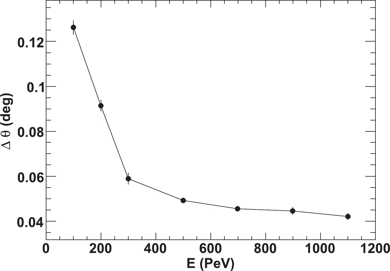
Figure 5. Width of the space angle distribution between the vector
$\vec{V_{C}}$ and the SDP of FD2 (or FD3).$ \chi^2_t = \sum \limits_{i = 1}^{N} \frac{(T_i - T_{\exp}(i))^2}{\sigma_i^2}, $

(7) where i represents the
$ i^{\rm th} $ SiPM of FD1,$ T_i $ is the observed triggering time, and$ \sigma_i $ is the width of the signal pulse.$ T_{\exp}(i) $ is the expected triggering time:$ T_{\rm exp}(i) = T_0+\frac{1}{c}(R_i - R_0 + \gamma \cdot R_{0i}), $

(8) where c is the speed of light,
$ T_0 $ is the observed triggering time of a reference SiPM which is selected in the center of the shower track and with a strong signal, and$ \gamma $ equals 1 for$ T_{\exp}(i) > T_0 $ and -1 for$ T_{\exp}(i) < T_0 $ . A schematic diagram of its calculation is shown in Fig. 6. As shown in Fig. 6,$ R_i $ and$ R_0 $ are the lengths of lines DA and DB, which extend from the FD1 site to the shower axis along the direction of the$ i^{\rm th} $ and reference SiPMs, respectively. Their lengths vary with the rotation of the FD2 (or FD3) SDP around a vector along$ \vec{V_{C}} $ .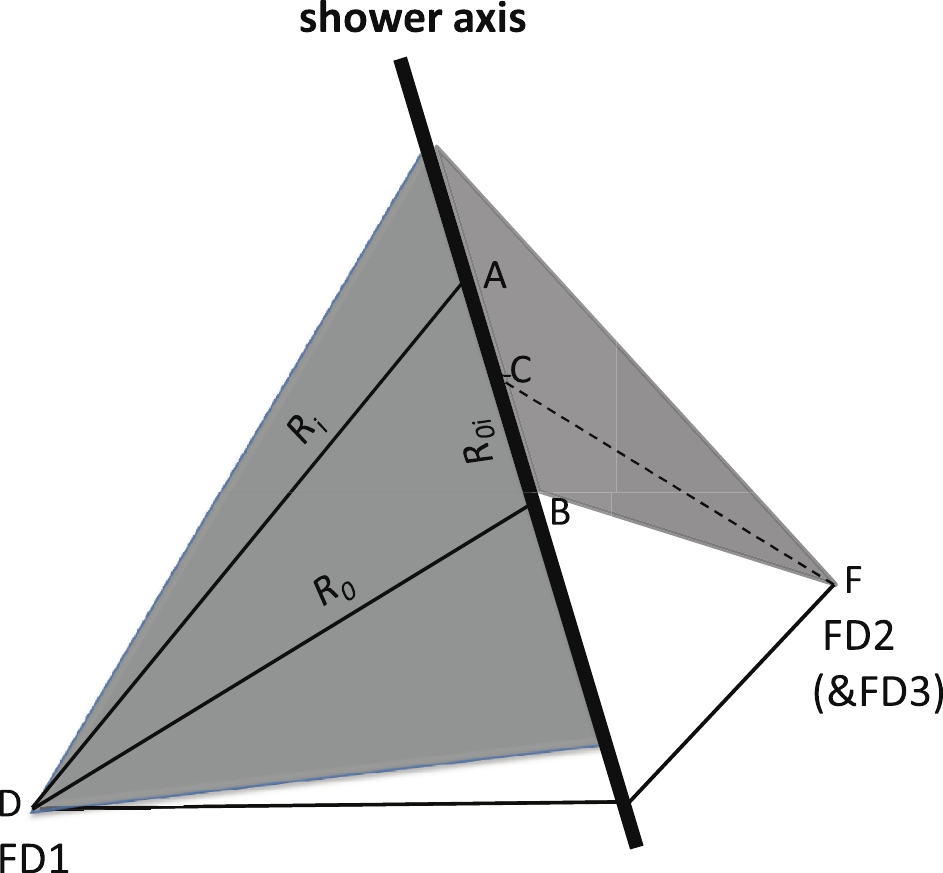
Figure 6. (color online) Schematic diagram of
$T_{\rm exp}$ calculation in stereo-timing fitting. Shaded areas represent the FOV of FD1 and FD2 (or FD3) respectively. DA and DB are lines from the FD1 site to the shower axis along the SiPM directions. FC is the central vector of the image observed by FD2 (or FD3).By minimizing
$ \chi_t^2 $ by changing the normal vector of SDP of FD2 (or FD3), one can obtain the true SDP. -
To have good resolution, events with poor reconstruction accuracy are cut with the following selections:
● Cut (i): Events falling in the edge of the FOV of the telescope array cannot be precisely reconstructed. To avoid such edge effects, an average vector for each event, weighted by the signals of the triggered SiPMs, i.e. the center of the image, is calculated. The minimal angular distances between the vector and the four FOV edges of the telescope array, called
$ \Delta \theta_t $ ,$ \Delta \theta_b $ ,$ \Delta \theta_l $ and$ \Delta \theta_r $ , are calculated. A parameter$ \Delta \theta $ which represents the minimal value of$ \Delta \theta_t $ ,$ \Delta \theta_b $ ,$ \Delta \theta_l $ and$ \Delta \theta_r $ , is applied. Events with$ \Delta \theta < 2^{\circ} $ (FD1) or$ \Delta\theta < 3^{\circ} $ (FD2 (or FD3)) are treated as marginal events and will be cut.● Cut (ii): For SDP reconstruction with the stereo-angular method, its resolution is significantly affected by the track length of the event. Thus, only events with track lengths greater than
$ 16^{\circ} $ in FD1 and greater than$ 14^{\circ} $ in FD2 (or FD3) are chosen for stereo-angular fitting. The resolution of the SDP of FD2 (or FD3) does not depend on the track length in stereo-timing fitting, and thus, it has no cut on the track length of FD2 (or FD3).● Cut (iii): Due to the fact that the shower trajectory is obtained by the intersection of two SDPs of FD1 and FD2 (or FD3), the trajectory cannot be reconstructed accurately if the opening angle of the two SDPs is either too small or too large; hence, a parameter
$ \Delta \phi $ is defined to describe this opening angle and events with$ \Delta \phi <10 ^{\circ} $ or$ \Delta \phi >170 ^{\circ} $ are rejected.The above event cuts are optimized considering both the improvement of reconstructed accuracy and the event survival rate. Figure 7 shows the event survival rate after each cut, which indicates that after all cuts, more than 48% of events remain in the stereo-angular method, and 57% of events in the stereo-timing method.
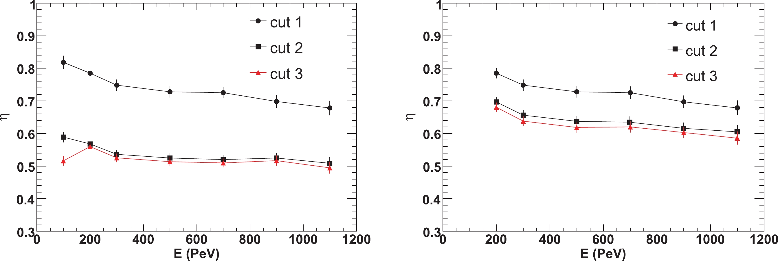
Figure 7. (color online) Event retention rate after Cut (i) (solid circles), Cut (i) + Cut (ii) (solid squares) and all cuts (solid triangles) at each energy for stereo-angular fitting (left) and stereo-timing fitting (right).
-
From the medians of the SDP reconstruction errors displayed in Table 3, it can be seen that FD1 has the best SDP resolution. For FD2 (or FD3), the SDP resolution with the stereo-timing method is better than that with the stereo-angular method. Taking the energy of 500 PeV as an example, their medians are
$ 0.064^{\circ} $ for FD1, and$ 0.366^{\circ}$ for FD2 (or FD3) with angular fitting (FD2_A), and$ 0.209^{\circ} $ for FD2 (or FD3) with timing fitting (FD2_T).Parameter Values E/PeV 100 200 300 500 700 900 1100 FD1/ $(^{\circ})$ 

0.210 0.116 0.089 0.064 0.060 0.056 0.052 FD2_A/ $(^{\circ})$ 

1.032 0.756 0.536 0.366 0.360 0.348 0.307 FD2_T/ $(^{\circ})$ 

− 0.737 0.310 0.209 0.201 0.182 0.156 Table 3. Medians of the distributions of the SDP reconstruction errors. FD2_A and FD2_T represent the errors obtained by the stereo-angular and stereo-timing method, respectively. For 100 PeV showers, the fluorescent light signal is too small, leading to a large error on the SiPM triggering times, so the SDP resolution of FD2 (or FD3) is too bad at this energy and is not recorded in the table.
Once the SDPs are obtained, reconstruction of the shower's primary direction is straightforward. By intersecting two SDPs from FD1 and FD2 (or FD3), the shower trajectory, and therefore its primary direction, can be obtained:
$ \overrightarrow{V_s}(m_s,n_s,l_s) = \overrightarrow{V_1}(m_1,n_1,l_1)\times\overrightarrow{V_2}(m_2,n_2,l_2), $

(9) where
$ \overrightarrow{V_1}(m_1,n_1,l_1) $ and$ \overrightarrow{V_2}(m_2,n_2,l_2) $ are the SDP normal vectors of FD1 and FD2 (or FD3) respectively.As an example, the distribution of the space angle between the reconstructed and the real shower directions at 500 PeV is shown in Fig. 8. They have quasi-two-dimensional Gaussian distributions and the medians of the distributions are taken to present the reconstruction accuracy. The medians as a function of energy after each cut are shown in Fig. 9 for the two reconstruction methods, and the final reconstruction accuracies after all cuts are shown in Fig. 10 and Table 4. The results indicate that at all energies, the stereo-timing method has better reconstruction ability than the stereo-angular method. Taking 500 PeV showers as an example, the angular resolutions are
$ 0.44^{\circ} $ and$ 0.23^{\circ} $ for the stereo-angular and stereo-timing methods, respectively. Figure 11 shows the event retention rates after all cuts. In stereo-timing fitting, the track length of the image of FD2 (or FD3) is not required to be greater than$ 14^{\circ}$ in the event selection. Therefore, its event retention rates are slightly higher than those in stereo-angular fitting.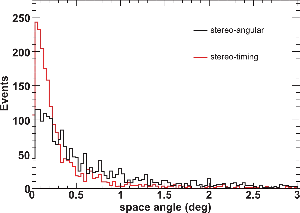
Figure 8. (color online) Distribution of space angle between reconstructed and simulated shower trajectories at 500 PeV for stereo-angular fitting (black curve) and stereo-timing fitting (red curve), respectively.

Figure 9. Distribution of space angle between reconstructed and actual shower trajectories after each cut at all energies for stereo-angular (left) and stereo-timing (right) methods, respectively.
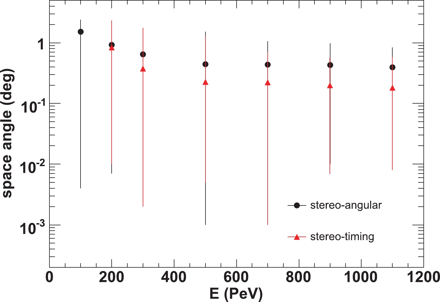
Figure 10. (color online) Distribution of space angle between reconstructed and actual shower trajectories after event selection at all energies for stereo-angular fitting (solid circles) and stereo-timing fitting (solid triangles), respectively. The 0-95% ranges of the distribution are also plotted (vertical lines).
Parameter Values E/PeV 100 200 300 500 700 900 1100 angular/ $(^{\circ})$ 

1.51 0.92 0.64 0.44 0.43 0.43 0.39 timing/ $(^{\circ})$ 

− 0.83 0.38 0.23 0.22 0.20 0.18 Table 4. Medians of the distributions of the shower direction reconstructed error for stereo-angular and stereo-timing techniques.
Figure 11. Event retention rates at each energy for stereo-angular fitting (solid triangles) and stereo-timing fitting (solid circles), respectively.
Once the trajectory is fixed, the impact parameter (Rp), which is the minimum distance from the site FD1 to the shower axis, can be calculated. Its reconstructed accuracy represented by both the relative and the absolute resolutions are shown in Tables 5 and 6 and Fig. 12. They indicate that the WFCTA also has good reconstruction ability in Rp and the resolution with stereo-timing fitting is also better than with stereo-angular fitting. For example, at 500 PeV, the relative resolutions are 0.41% for stereo-angular fitting and 0.25% for stereo-timing fitting. The absolute resolutions are 25.5 m for stereo-angular fitting and 14.3 m for stereo-timing fitting.
Parameter Values E/PeV 100 200 300 500 700 900 1100 angular (%) 0.91 0.59 0.53 0.41 0.39 0.39 0.28 timing (%) − 0.46 0.32 0.25 0.24 0.23 0.18 Table 5. Relative resolution of Rp (%) described by the standard deviation for stereo-angular and stereo-timing techniques.
Parameter Values E/PeV 100 200 300 500 700 900 1100 angular/m 63.6 44.8 31.9 25.5 25.1 23.5 22.0 timing/m − 27.5 21.6 14.3 13.8 13.5 13.3 Table 6. Absolute resolution of Rp (m) described by the standard deviation for stereo-angular and stereo-timing techniques.

Figure 12. Relative resolution (left) and absolute resolution (right) of Rp for stereo-angular fitting (solid circles), and stereo-timing fitting (solid triangles), respectively.
-
Errors in the geometry determination will contribute to errors in the reconstruction of shower energy and
$ X_{\max} $ . However, there are other uncertainty sources which are as important or more important. Measuring the energy and$ X_{\max} $ requires accurate determination of a shower's longitudinal development profile. Uncertainties in the profile are mainly from atmosphere attenuation uncertainty related to aerosol attenuation, calibration uncertainty, fluorescent light generation efficiency, and so on. These uncertainties will be discussed in detail in a future publication on energy and$ X_{\max} $ measurements.The uncertainty in shower geometry determination will introduce an error in the light attenuation from the shower to the detector in the energy measurement. For a distance error
$ \vartriangle r $ , the fractional change in the light attenuation is approximately$ {\rm e}^{\vartriangle r/\lambda} $ , where$ \lambda $ is the attenuation length of light. The average attenuation length is about 12 km at 350 nm [10]. Even with a distance error of 0.1 km, which is larger than the core error discussed in this paper, the resulting attenuation correction change is only about 1%. This is very small compared with the uncertainty in attenuation length itself (leading to an energy uncertainty of order 10%), and uncertainty in the detector calibration, which is also of the order of 10% [11].An error in the zenith angle of the shower axis can lead to an uncertainty in the position of
$ X_{\max} $ . Taking a typical shower with zenith angle of$ 45^{\circ} $ and$ X_{\max} $ of$ 750 \;{\rm{g/cm^2}} $ , an error of$ 1.5^{\circ} $ in this angle will lead to an error in$ X_{\max} $ of approximately$ 14 \;{\rm{g/cm^2}} $ . This is an extreme case because: 1) we consider the largest zenith angle error discussed in this paper; and 2) we derive all the zenith angle error from the error in$ \Psi $ , which is the angle of the shower axis in the SDP. In real measurements, the uncertainty of$ X_{\max} $ will be smaller than this estimation. -
In this study, the geometrical reconstruction of the WFCTA experiment in fluorescence observation mode was tested. First, the reconstruction principles of two approaches, the stereo-angular and stereo-timing methods, were described. The principle of the shower direction reconstruction in both these methods uses the intersection of two SDPs (from FD1 and FD2 (or FD3)); thus the fundamental issue is the reconstruction of the SDPs. Given the wider FOV and consequently longer tracks, FD1 has better performance in reconstructing the SPD (less than
$ 0.09^{{\circ}} $ above 300 PeV). For FD2 (or FD3), it is only less than$ 0.54^{{\circ}} $ above 300 PeV using the same reconstruction method as FD1 (stereo-angular method). However, for the SDP reconstruction with the stereo-timing method, which does not depend on the length of the shower tracks, their resolution can be as good as$ 0.31^{{\circ}} $ . With the described event selection, the WFCTA has good geometrical reconstruction ability in terms of both shower direction and shower distance. In addition, the geometrical resolution of the stereo-timing method is shown to be superior to that of the stereo-angular method. Above 500 PeV, the medians of the reconstruction error of the cosmic ray direction with the stereo-timing method are better than$ 0.23^{{\circ}} $ , and the relative resolution of Rp is better than 0.25%, whereas for the stereo-angular method these are$ 0.44^{{\circ}} $ and 0.41%, respectively. As well as the better geometrical resolution for the stereo-timing method, the acceptance of the telescope array is also increased by about 10%. This will decrease the statistical uncertainty, which is important since we focus on the measurement of ultra-high energy showers which only have low flux. Furthermore, geometry errors lead to an uncertainty component in the measurement of other shower parameters, like energy,$ X_{\max} $ . We have shown that the geometric accuracy is at a level that does not dominate these errors.
Geometrical reconstruction of fluorescence events observed by the LHAASO experiment
- Received Date: 2020-09-30
- Available Online: 2021-04-15
Abstract: The LHAASO-WFCTA experiment, which aims to observe cosmic rays in the sub-EeV range using the fluorescence technique, uses a new generation of high-performance telescopes. To ensure that the experiment has excellent detection capability associated with the measurement of the energy spectrum, the primary composition of cosmic rays, and so on, an accurate geometrical reconstruction of air-shower events is fundamental. This paper describes the development and testing of geometrical reconstruction for stereo viewed events using the WFCTA (Wide Field of view Cherenkov/Fluorescence Telescope Array) detectors. Two approaches, which take full advantage of the WFCTA detectors, are investigated. One is the stereo-angular method, which uses the pointing of triggered SiPMs in the shower trajectory, and the other is the stereo-timing method, which uses the triggering time of the fired SiPMs. The results show that both methods have good geometrical resolution; the resolution of the stereo-timing method is slightly better than the stereo-angular method because the resolution of the latter is slightly limited by the shower track length.


 DownLoad: