


 Abstract
 HTML
HTML Reference
 Related
 PDF
PDF


-
The observed neutrino oscillation data, including the neutrino mass-squared differences, mixing angles, and the Dirac CP phases given in Table 1, is a subject of intense interest in current particle physics. This pattern provides inspiration for constructing models with additional scalars and symmetries and makes it interesting to extend the SM. Among the various extensions of the SM, the
$ B-L $ gauge model is one of the simplest extensions which has been studied in previous works [2-12], whereby the anomalies are canceled in different ways [13-15]①. In this work, we improve the model proposed in Refs. [7, 8], where neutrino masses and various other phenomena involving leptogenesis, dark matter, etc, are satisfied. It is emphasized that the above-mentioned model by itself cannot predict the recently observed neutrino oscillation data.Parameters NH IH $ {\rm{bfp}}\pm 1 \sigma $ 

$ 3 \sigma $ range

$ {\rm{bfp}}\pm 1 \sigma $ 

$ 3 \sigma $ range

$ \sin^2\theta_{23} $ 

$ 0.573_{-0.020}^{+0.016} $ 

$ 0.415 \to 0.616 $ 

$ 0.575_{-0.019}^{+0.016} $ 

$ 0.419 \to 0.617 $ 

$\theta_{23}/(^\circ)$ 

$ 49.2_{-1.2}^{+0.9} $ 

$ 40.1 \to 51.7 $ 

$ 49.3_{-1.1}^{+0.9} $ 

$ 40.3 \to 51.8 $ 

$ \sin^2\theta_{12} $ 

$ 0.304_{-0.012}^{+0.012} $ 

$ 0.269 \to 0.343 $ 

$ 0.304_{-0.012}^{+0.013} $ 

$ 0.269 \to 0.343 $ 

$\theta_{12}/(^\circ)$ 

$ 33.44_{-0.74}^{+0.77} $ 

$ 31.27 \to 35.86 $ 

$ 33.45_{-0.75}^{+0.78} $ 

$ 31.27 \to 35.87 $ 

$ \sin^2\theta_{13} $ 

$ 0.02219_{-0.00063}^{+0.00062} $ 

$ 0.02032 \to 0.02410 $ 

$ 0.02238_{-0.00062}^{+0.00063} $ 

$ 0.02052 \to 0.02428 $ 

$\theta_{13}/(^\circ)$ 

$ 8.57_{-0.12}^{+0.12} $ 

$ 8.20 \to 8.93 $ 

$ 8.60_{-0.12}^{+0.12} $ 

$ 8.24 \to 8.96 $ 

$\delta _{\rm CP}(^\circ)$ 

$ 197_{-24}^{+27} $ 

$ 120 \to 369 $ 

$ 282_{-30}^{+26} $ 

$ 193 \to 352 $ 

$\dfrac{ \Delta m^2_{21} }{10^{-5}\, {\rm{eV} }^2}$ 

$ 7.42_{-0.20}^{+0.21} $ 

$ 6.82 \to 8.04 $ 

$ 7.42_{-0.20}^{+0.21} $ 

$ 6.82 \to 8.04 $ 

$\dfrac{ \Delta m^2_{3 l} }{10^{-3}\, {\rm{eV} }^2}$ 

$ +2.517_{-0.028}^{+0.026} $ 

$ +2.435 \to +2.598 $ 

$ -2.498_{-0.028}^{+0.028} $ 

$ -2.581 \to -2.414 $ 

Table 1. Observed neutrino oscillation data taken from Ref. [1]. Here,
$ \Delta m^2_{3l}\equiv \Delta m^2_{31} >0 $ for NH and$ \Delta m^2_{3l}\equiv \Delta m^2_{32} < 0 $ for IH.It is worth mentioning that non-Abelian discrete symmetries have revealed many outstanding issues. Consequently, many of them have been applied in explaining the observed neutrino oscillation pattern. One of them, the
$ S_{4} $ symmetry, has been widely used because it provides a viable description of the observed neutrino oscillation data [15-41]. However, the above-mentioned models contain non-minimal scalar sectors with many Higgs doublets. Thus, it is interesting to find an alternative extension which can give a better explanation of the observed neutrino oscillation data with less scalar content than previous models. In this work, we propose an alternative and improved version of the$ B-L $ model with an additional flavor symmetry group,$ S_4\otimes Z_{3} $ , which accommodates the current neutrino oscillation data given in Table 1. In this work, all left-handed leptons are put in$ \underline{3} $ while for the right-handed leptons, the first generation is put in$ \underline{1} $ and the two others are in$ \underline{2} $ . The$ S_4 $ group contains 24 elements dispensed into five conjugacy classes and five irreducible representations, denoted as$ \underline{1},\; \underline{1}^{'} $ ,$ \underline{2}, \;\underline{3} $ , and$ \underline{3}^{'} $ . In this paper, we work in the basis where$ \underline{3} $ and$ \underline{3}^{'} $ are real whereas$ \underline{2} $ is complex. For a detailed description of the$ S_4 $ group, the reader is referred to Ref. [15]. Despite the$ S_4 $ symmetry being previously studied in various works [15-41], to the best of our knowledge, this symmetry has not been considered before in the$ B-L $ scenario.This paper is arranged as follows. The model is described in Section II. Section III is devoted to neutrino mass and mixing. The results of the numerical analysis are presented in Section IV and finally, some conclusions are given in Section V.
-
The full symmetry of the model is
$ G = G_{\rm SM}\otimes U(1)_{B-L}\otimes S_4\otimes Z_3 $ , where$ G_{\rm SM} = SU(3)_{\rm C} \otimes SU(2)_{\rm L} \otimes U(1)_{\rm Y} $ is the gauge group of the SM. In this model, the first generation of right-handed leptons is put in$ \underline{1} $ while the two others are put in$ \underline{2} $ under$ S_4 $ and the three generations of left-handed leptons as well as the three right-handed neutrinos are put in$ \underline{3} $ . The model particle content is given in Table 2, where$ \phi, \phi^{'} $ and$ \eta $ are$ S_4 $ triplets whose components are$ SU(2)_{\rm L} $ singlets, and$ \chi $ is one$ S_4 $ doublet whose components are$ SU(2)_{\rm L} $ singlets.Fields $ \psi_{\rm L} $ 

$ l_{1{\rm R}} (l_{ \alpha {\rm R}}) $ 

$ \nu_{\rm R} $ 

H $ \phi $ 

$ \phi^{'} $ 

$ \chi $ 

$ \eta $ 

$ SU(3)_{\rm C} $ 

$ {\bf{1}} $ 

$ {\bf{1}} $ 

$ {\bf{1}} $ 

$ {\bf{1}} $ 

$ {\bf{1}} $ 

$ {\bf{1}} $ 

$ {\bf{1}} $ 

$ {\bf{1}} $ 

$ SU(2)_{\rm L} $ 

$ {\bf{2}} $ 

$ {\bf{1}} $ 

$ {\bf{1}} $ 

$ {\bf{2}} $ 

$ {\bf{1}} $ 

$ {\bf{1}} $ 

$ {\bf{1}} $ 

$ {\bf{1}} $ 

$U(1)_{\rm Y}$ 

$ - \frac{1}{2} $ 

$ -1 $ 

$ 0 $ 

$ \frac{1}{2} $ 

$ 0 $ 

$ 0 $ 

$ 0 $ 

$ 0 $ 

$ U(1)_{B-L} $ 

$ -1 $ 

$ -1 $ 

$ -1 $ 

$ 0 $ 

$ 0 $ 

$ 0 $ 

$ 2 $ 

$ 2 $ 

$ S_4 $ 

$ \underline{3} $ 

$ \underline{1} (\underline{2}) $ 

$ \underline{3} $ 

$ \underline{1} $ 

$ \underline{3} $ 

$ \underline{3}^{'} $ 

$ \underline{2} $ 

$ \underline{3} $ 

$ Z_3 $ 

$ \omega^2 $ 

$ \omega $ 

$ \omega^2 $ 

$ 1 $ 

$ \omega $ 

$ \omega $ 

$ \omega^2 $ 

$ \omega^2 $ 

Table 2. The model particle and scalar contents (
$ \alpha = 2,3 $ ).Under G symmetry,
$ \bar{\psi}_{\rm L} l_{1{\rm R}} $ and$ \bar{\psi}_{\rm L} l_{ \alpha {\rm R}} $ transform as$ (1, 2, -1/2, 0, \underline{3}, \omega^2) $ and$ (1, 2, -1/2, 0, \underline{3}\oplus \underline{3}^{'} , \omega^2) $ , respectively. Thus, we need one$ SU(2)_{\rm L} $ doublet H and two$ SU(2)_{\rm L} $ singlets$ \phi, \phi^{'} $ , as presented in Table 2, to generate masses for the charged leptons.Furthermore, the neutrino masses arise from
$ \bar{\psi}_{\rm L} \nu_{\rm R} $ and$ \bar{\nu}^c_{\rm R} \nu_{\rm R} $ to scalars, where under G symmetry,$ \bar{\psi}_{\rm L} \nu_{\rm R}\sim (1,2,1/2, 0, \underline{1} \oplus \underline{2}\oplus \underline{3}\oplus \underline{3}^{'}, 1) $ and$ \bar{\nu}^c_{\rm R} \nu_{\rm R}\sim (1, 1,0, -2, \underline{1} \oplus \underline{2}\oplus \underline{3}\oplus \underline{3}^{'} , \omega) $ . For the known scalars ($ H, \phi, \phi^{'} $ ), under G symmetry, there is only one invariant term$ (\bar{\psi}_{\rm L} \nu_{\rm R})_{\underline{1}}\widetilde{H} $ which is responsible for generating Dirac masses for the neutrinos. In order to generate realistic neutrino masses and mixings, we add two singlets$ \chi, \eta $ , respectively put in$ \underline{2} $ and$ \underline{3} $ under$ S_4 $ coupling to$ \bar{\nu}^c_{\rm L}\nu_{\rm R} $ which are responsible for generating Majorana masses for the neutrinos.Up to five dimensions, the Yukawa couplings invariant under all symmetries are②
$ \begin{aligned}[b] -{\cal{L}}_{l} =& \frac{h_1}{ \Lambda } (\bar{\psi}_{\rm L} l_{1{\rm R}})_{\underline{3}} (H\phi)_{\underline{3}}+ \frac{h_2}{ \Lambda } (\bar{\psi}_{\rm L} l_{ \alpha {\rm R}})_{\underline{3}} (H\phi)_{\underline{3}} \\&+ \frac{h_3}{ \Lambda } (\bar{\psi}_{\rm L} l_{ \alpha {\rm R}})_{\underline{3}^{'}} (H\phi^{'})_{\underline{3}^{'}} + x (\bar{\psi}_{\rm L} \nu_{\rm R})_{\underline{1}}\widetilde{H}\\&+ \frac{y}{2} (\bar{\nu}^c_{\rm R} \nu_{\rm R})_{\underline{2}}\chi + \frac{z}{2} (\bar{\nu}^c_{\rm R} \nu_{\rm R})_{\underline{3}}\eta+{\rm H.c}, \end{aligned} $

(1) where
$ \Lambda $ is the cut-off scale of the theory, and$ h_{1,2,3} $ as well as$ x, \;y,\; z $ are the dimensionless Yukawa coupling constants.To generate a suitable neutrino oscillation pattern, the following structure of VEVs is chosen:
$ \begin{aligned}[b] \langle H \rangle^T =& ( 0 v_H) , \langle \phi \rangle = (\langle \phi_1 \rangle,\langle \phi_1 \rangle, \langle \phi_1 \rangle),\langle \phi_1 \rangle = v_\phi, \\ \langle \phi^{'} \rangle =& (\langle \phi^{'}_1 \rangle,\langle \phi^{'}_1 \rangle,\langle \phi^{'}_1 \rangle), \langle \phi^{'}_1 \rangle = v_{\phi^{'}},\\ \langle \eta \rangle =& (0,0, \langle \eta_3 \rangle) ,\langle \eta_3 \rangle = v_\eta, \\ \langle \chi \rangle =& (\langle \chi_1 \rangle,\langle \chi_2 \rangle),\langle \chi_{1,2} \rangle = v_{\chi_{1,2}}. \end{aligned} $

(2) The VEVs of
$ \phi $ and$ \phi^{'} $ , respectively, break$ S_4 $ down to$ S_3 $ and$ Z_3 $ , while the VEVs of$ \chi $ and$ \eta $ break$ S_4 $ down to the Klein four group$ K_4 $ .From Eq. (1), with expansion
$ \phi_i = \langle \phi_i\rangle +\phi^{'}_i $ and$ H = (H^+ H^0)^T $ , we get the lepton flavor changing interactions:$ \begin{aligned}[b] -{\cal{L}}_{\rm clep}\supset &\frac{h_1 v_{\phi}}{ \Lambda }(\bar{l}_{\rm 2L}H^0 + \bar{\nu}_{2{\rm L}}H^+) l_{1{\rm R}} + \frac{h_1 v_{\phi}}{ \Lambda }(\bar{l}_{\rm 3L}H^0\\ & +\bar{\nu}_{\rm 3L}H^+) l_{\rm 1R} + \frac{h_2 v_{\phi}}{ \Lambda } (\bar{l}_{\rm 1L}H^0+ \bar{\nu}_{\rm 1L}H^+)l_{\rm 2R}\\ & + \frac{h_2 v_{\phi}}{ \Lambda } (\bar{l}_{\rm 1L}H^0 + \bar{\nu}_{\rm 1L}H^+)l_{\rm 3R} - \frac{h_3 v_{\phi^{'}}}{ \Lambda }(\bar{l}_{\rm 1L}H^0 \\ &+ \bar{\nu}_{\rm 1L}H^+)l_{\rm 2R} + \frac{h_3 v_{\phi^{'}}}{ \Lambda }(\bar{l}_{\rm 1L}H^0 + \bar{\nu}_{\rm 1L}H^+)l_{\rm 3R} + {\rm H.c} \, . \end{aligned} $

(3) Equation (3) shows that, in the case
$ v_{\phi^{'}}\simeq v_{\phi} $ , the usual Yukawa couplings are proportional to$ \dfrac{v_{\phi}}{ \Lambda} $ and the lepton flavor changing processes in this model are suppressed by the factor③$ \dfrac{v_{\phi}}{ \Lambda G_F^2M_H^2} $ associated with the above small Yukawa couplings and the large mass scale of the heavy scalars. For further details, the reader is referred to Refs. [42-45]. Furthermore, this model contains only one$ SU(2)_{\rm L} $ Higgs doublet; therefore, the flavor changing neutral current processes are absent at tree level. -
From the Yukawa interactions in Eq. (1), using the tensor product of
$ S_4 $ [15], together with the VEVs of H,$ \phi $ and$ \phi^{'} $ in Eq. (2), the charged lepton mass terms are written as follows:$ {\cal{L}}^{\rm{mass}}_{cl} = - (\bar{l}_{\rm 1L} \bar{l}_{\rm 2L} \bar{l}_{\rm 3L}) M_l (l_{\rm 1R} l_{\rm 2R} l_{\rm 3R})^T+{\rm H.c}, $

(4) where
$ {M_l} = \frac{{{v_H}}}{\Lambda }\left( {\begin{array}{*{20}{c}} {{h_1}{v_\phi }}&{{h_2}{v_\phi } - {h_3}{v_{\phi '}}}&{{h_2}{v_\phi } + {h_3}{v_{\phi '}}}\\ {{h_1}{v_\phi }}&{{\omega ^2}({h_2}{v_\phi } - {h_3}{v_{\phi '}})}&{\omega ({h_2}{v_\phi } + {h_3}{v_{\phi '}})}\\ {{h_1}{v_\phi }}&{\omega ({h_2}{v_\phi } - {h_3}{v_{\phi '}})}&{{\omega ^2}({h_2}{v_\phi } + {h_3}{v_{\phi '}})} \end{array}} \right).$

(5) The matrix
$ M_l $ is diagonalized as$ U^\dagger_l M_l U_r = {\rm{diag}}(m_e, \, m_\mu , \,m_\tau) $ , where$ \begin{array}{*{20}{l}} {U_{\rm L}^\dagger = \dfrac{1}{{\sqrt 3 }}\left( {\begin{array}{*{20}{c}} 1&{ 1}&{ 1}\\ 1&{ \omega }&{ {\omega ^2}}\\ 1&{ {\omega ^2}}&{ \omega } \end{array}} \right),\;\;\;{U_{\rm R}} = {I_{3 \times 3}},\;\;\;\omega = {{\rm e}^{{\rm i}2\pi /3}},} \end{array}$

(6) $ m_e = \frac{\sqrt{3} h_1 v_H v_{\phi}}{ \Lambda },\;\;\; m_{\mu,\tau} = \frac{\sqrt{3}v_H}{ \Lambda } \left(h_2v_{\phi} \mp h_3v_{\phi^{'}}\right). \ $

(7) The left-handed mixing matrix
$ U_{\rm L} $ is non-trivial in our model and hence will contribute to the leptonic mixing matrix. Equation (7) shows that$ m_{\mu} $ and$ m_{\tau} $ are differentiated by$ \phi^{'} $ . This is why$ \phi^{'} $ is additionally introduced to$ \phi $ in the charged-lepton sector. Now, comparing the result in Eq. (7) with the best fit values for the masses of charged leptons taken from Ref. [46],$ m_e \simeq 0.511 \; \rm{MeV} $ ,$ \, m_\mu \simeq 105.66 \; \rm{MeV} $ , and$ \, m_\tau \simeq 1776.86 \; \rm{MeV} $ , we find the relations$ \dfrac{h_1 v_{H} v_\phi}{ \Lambda } = 0.295\; {\rm{MeV}},\; \dfrac{h_2 v_{H} v_\phi}{ \Lambda } = 543\; {\rm{MeV}},\; \dfrac{h_3 v_{H} v_{\phi^{'}}}{ \Lambda } = 482\, {\rm{MeV}},\; {\rm i.e.},\; h_1:h_2:h_3\sim 1.00: 1.840\times 10^3: 1.634\times 10^3 $ .Regarding the neutrino sector, from the Yukawa terms in Eq. (1) and using the tensor product of
$ S_4 $ [15], the Yukawa Lagrangian invariant under G symmetry in the neutrino sector reads:$ \begin{aligned}[b] -{\cal{L}}_{\nu} = & x \left(\bar{\psi}_{\rm 1L} \nu_{\rm 1R} +\bar{\psi}_{\rm 2L} \nu_{\rm 2R} +\bar{\psi}_{\rm 2L} \nu_{\rm 3R} \right)\widetilde{H} \\ & + \frac{y}{2} \left[(\chi_1+\chi_2)\bar{\nu}^c_{\rm 1R}\nu_{\rm 1R} + \omega( \omega \chi_1+ \chi_2)\bar{\nu}^c_{\rm 2R}\nu_{\rm 2R} \right.\\& \left.+ \omega(\chi_1+ \omega \chi_2)\bar{\nu}^c_{\rm 3R}\nu_{\rm 3R}\right] \\ & +\frac{z}{2} \left[(\bar{\nu}^c_{\rm 2R}\nu_{\rm 3R}+\bar{\nu}^c_{\rm 3R}\nu_{\rm 2R})\eta_1+(\bar{\nu}^c_{\rm 3R}\nu_{\rm 1R}+\bar{\nu}^c_{\rm 1R}\nu_{\rm 3R})\eta_2 \right.\\&+(\bar{\nu}^c_{\rm 1R}\nu_{\rm 2R} +\bar{\nu}^c_{\rm 2R}\nu_{\rm 1R})\eta_3 \Big] + {\rm H.c}. \end{aligned} $

(8) After symmetry breaking, the mass Lagrangian for the neutrinos takes the following form:
$ -{\cal{L}}^{\rm mass}_{\nu} = \frac 1 2 \bar{\chi}^c_{\rm L} M_\nu \chi_{\rm L}+ {\rm H.c}, $

(9) where
$\begin{aligned}[b] &{{\chi _{\rm L}} = {{\left( {{\nu _{\rm L}}\;\;\nu _{\rm R}^c} \right)}^T},\;\;\;{M_\nu } = \left( {\begin{array}{*{20}{c}} 0&{M_D^T}\\ {{M_D}}&{{M_{\rm R}}} \end{array}} \right),}\\ &{{\nu _{\rm L}} = {{({\nu _{\rm 1L}}\;\;{\nu _{\rm 2L}}\;\;{\nu _{\rm 3L}})}^T},\;\;\;\nu _{\rm R}^c = {{(\nu _{\rm 1R}^c\;\;\nu _{\rm 2R}^c\;\;\nu _{\rm 3R}^c)}^T},} \end{aligned} $

(10) and the mass matrices
$ M_D, \;M_{\rm R} $ take the following forms:$ \begin{aligned}[b] {{M_D} = &{\rm{diag}}({a_D},{a_D},{a_D}),\\ {M_{\rm R}} =& \left( {\begin{array}{*{20}{c}} {{a_{\rm 1R}} + {a_{\rm 2R}}}&{{a_{\rm R}}}&0\\ {{a_{\rm R}}}&{\omega (\omega {a_{\rm 1R}} + {a_{\rm 2R}})}&0\\ 0&0&{\omega ({a_{\rm 1R}} + \omega {a_{\rm 2R}})} \end{array}} \right),} \end{aligned} $

(11) where
$ a_D = x v^*_{\phi}, \,\,\;\;\;\;\; a_{1,2 {\rm R}} = y v_{\chi_{1,2}},\,\, \;\;\;\;\;a_{\rm R} = z v_\eta. $

(12) In the seesaw mechanism, the effective neutrino mass matrix is given by
$ {M_{{\rm{eff}}}} = - M_D^TM_R^{ - 1}{M_D} = \left( {\begin{array}{*{20}{c}} {{A_1} + i{A_2}}&{{A_7} + i{A_8}}&0\\ {{A_7} + i{A_8}}&{{A_3} + i{A_4}}&0\\ 0&0&{{A_5} + i{A_6}} \end{array}} \right), $

(13) where
$ \begin{aligned}[b] A_1 A_0 =& -\left[2 (a_{\rm 1R}^3 + a_{\rm 2R}^3) + (a_{\rm 1R} + a_{\rm 2R}) a_{\rm R}^2\right]a_D^2, \\ A_2 A_0 =& \sqrt{3} (a_{\rm 2R}-a_{\rm 1R}) a_D^2 a_{\rm R}^2, \\ A_3 A_0 =& (a_{\rm 1R} + a_{\rm 2R}) a_D^2 [(a_{\rm 1R} + a_{\rm 2R})^2 + 2 a_{\rm R}^2], \\ A_4 A_0 = &\sqrt{3} (a_{\rm 2R} - a_{\rm 1R}) (a_{\rm 1R} + a_{\rm 2R})^2 a_D^2, \\ A_5 =& \frac{(a_{\rm 1R} + a_{\rm 2R}) a_D^2}{2\left(a_{\rm 1R}^2 - a_{\rm 1R} a_{\rm 2R} + a_{\rm 2R}^2\right)}, \\ A_6 = &\frac{\sqrt{3}}{2} \frac{(a_{\rm 2R}-a_{\rm 1R}) a_D^2}{a_{\rm 1R}^2 - a_{\rm 1R} a_{\rm 2R} + a_{\rm 2R}^2}, \\ A_7 A_0 =& -a_D^2 a_{\rm R} \left[(a_{\rm 1R} + a_{\rm 2R})^2 + 2 a_{\rm R}^2\right], \\ A_8 A_0 =& \sqrt{3} (a_{\rm 1R}^2-a_{\rm 2R}^2) a_D^2 a_{\rm R}, \\ A_0 =& 2 \Big[a_{\rm 1R}^4 + a_{\rm 1R}^3 a_{\rm 2R} \\&+ a_{\rm 1R} a_{\rm 2R}^3 + a_{\rm 2R}^4 + (a_{\rm 1R} + a_{\rm 2R})^2 a_{\rm R}^2 + a_{\rm R}^4\Big]. \end{aligned} $

(14) Let us first define a Hermitian matrix
$ {\cal{M}}^2 $ , given by$ {M^2} = {M_{{\rm{eff}}}}M_{{\rm{eff}}}^ + = \left( {\begin{array}{*{20}{c}} {{a_0}}&{{d_0} + {\rm i}{g_0}}&0\\ {{d_0} - {\rm i}{g_0}}&{{b_0}}&0\\ 0&0&{{c_0}} \end{array}} \right), $

(15) where
$ \begin{aligned}[b] a_0 =& a_1^2 + a_2^2 + a_7^2 + a_8^2 + 2 a_1 a_2 \sin( \alpha _1- \alpha _2) \\&+ 2 a_7 a_8 \sin( \alpha _7- \alpha _8), \\ b_0 =& a_3^2 + a_4^2 + a_7^2 + a_8^2 + 2 a_3 a_4 \sin( \alpha _3- \alpha _4) \\&+ 2 a_7 a_8 \sin( \alpha _7- \alpha _8), \\ c_0 =& a_5^2 + a_6^2 + 2 a_5 a_6 \sin( \alpha _5- \alpha _6),\\ d_0 =& a_7 [a_1 \cos( \alpha _1- \alpha _7)- a_2 \sin( \alpha _2- \alpha _7)\\&+ a_3 \cos( \alpha _3- \alpha _7)+a_4 \sin( \alpha _4- \alpha _7)] \\& +\, a_8 [a_1 \sin( \alpha _1- \alpha _8)+a_2 \cos( \alpha _2- \alpha _8)\\& + a_3 \sin( \alpha _3- \alpha _8)+ a_4 \cos( \alpha _4- \alpha _8)], \\ g_0 =& a_7[a_1 \sin( \alpha _1- \alpha _7)+a_2\cos( \alpha _2- \alpha _7) \\&-a_3 \cos( \alpha _3- \alpha _7)-a_4 \sin( \alpha _4- \alpha _7)] \\& -\, a_8[a_1 \cos( \alpha _1- \alpha _8)-a_2 \sin( \alpha _2- \alpha _8)\\&-a_3 \cos( \alpha _3- \alpha _8)+ a_4\sin( \alpha _4- \alpha _8)], \end{aligned} $

(16) with
$ a_i = |A_i| $ and$ \alpha _i\, (i = 1-8) $ being the arguments of$ A_i $ .The squared-mass matrix
$ {\cal{M}}^2 $ in Eq. (15) has three exact eigenvalues:$ m_1 = \kappa _1- \kappa _2,\;\; m_2 = c_0, \;\;m_{3} = \kappa _1+ \kappa _2, $

(17) with
$ 2 \kappa _1 = a_0 + b_0, \;\;2 \kappa _2 = \sqrt{(a_0 - b_0)^2 + 4 (d_0^2 + g_0^2)}, $

(18) and the corresponding mixing matrix is
$U= \left( {\begin{array}{*{20}{c}} {{\rm{cos}}\theta }&0&{ - \sin \theta {\mkern 1mu} {{\rm e}^{{\rm i}\alpha }}}\\ 0&1&0\\ {{\rm{sin}}\theta {{\rm e}^{ - {\rm i}\alpha }}}&0&{\cos \theta } \end{array}} \right),$

(19) with
$ \begin{aligned}[b] \alpha =& -{\rm i}\ln\left(- \frac{d_0 +{\rm i} g_0}{\sqrt{d^2_0 + g^2_0}}\right),\\ \theta =& \arcsin\left( \frac{1}{K^2+1}\right),\end{aligned}$

(20) $ K = \frac{b_0-m_1}{\sqrt{d_0^2 + g_0^2}} = \frac{m_3-a_0}{\sqrt{d_0^2 + g_0^2}}. $

(21) The sign of
$ \Delta m^2_{31} $ plays a pivotal role in the form of the neutrino mass hierarchy. In the NH,$ m_1\ll m_{2}\sim m_{3} $ , and thus the lightest neutrino mass is$ m_1 $ , while in the IH,$ m_3\ll m_1\sim m_2 $ , thus the lightest neutrino mass is$ m_3 $ [46]. The neutrino mass matrix$ {M}_{\rm{eff}} $ in Eq. (13) is diagonalized as$U_\nu ^ + {{\cal{M}}^2}{U_\nu } = \left\{ {\begin{array}{*{20}{l}} {\left( {\begin{array}{*{20}{c}} {{m_1}}&0&0\\ 0&{{m_2}}&0\\ 0&0&{{m_3}} \end{array}} \right),\;{U_\nu } = \left( {\begin{array}{*{20}{c}} {{\rm{cos}}\theta }&0&{ - {\rm{sin}}\theta {\mkern 1mu} {{\rm e}^{{\rm i}\alpha }}}\\ {{\rm{sin}}\theta {{\rm e}^{ - {\rm i}\alpha }}}&0&{{\rm{cos}}\theta }\\ 0&1&0 \end{array}} \right)\;\;{\rm{for}}\;{\rm{NH,}}\;\;}\\ {\left( {\begin{array}{*{20}{c}} {{m_3}}&0&0\\ 0&{{m_2}}&0\\ 0&0&{{m_1}} \end{array}} \right),\;{U_\nu } = \left( {\begin{array}{*{20}{c}} {{\rm{sin}}\theta {\mkern 1mu} {{\rm e}^{{\rm i}\alpha }}}&0&{{\rm{cos}}\theta }\\ { - {\rm{cos}}\theta }&0&{{\rm{sin}}\theta {{\rm e}^{ - {\rm i}\alpha }}}\\ 0&1&0 \end{array}} \right)\;\;{\rm{for}}\;{\rm{IH,}}} \end{array}} \right. $

(22) where
$ m_{2,3} $ and$ \alpha , \theta $ are given in Eqs. (17) and (20), respectively. The corresponding leptonic mixing matrix is$ {U_{\rm lep}} = U_{\rm L}^\dagger {U_\nu } = \left\{ {\begin{array}{*{20}{l}} {\dfrac{1}{{\sqrt 3 }}\left( {\begin{array}{*{20}{c}} {\cos \theta + \sin \theta .{{\rm e}^{ - {\rm i}\alpha }}}&1&{\cos \theta - \sin \theta .{{\rm e}^{{\rm i}\alpha }}}\\ {\cos \theta + \omega \sin \theta .{{\rm e}^{ - {\rm i}\alpha }}}&{{\omega ^2}}&{\omega \cos \theta - \sin \theta .{{\rm e}^{{\rm i}\alpha }}}\\ {\cos \theta + {\omega ^2}\sin \theta .{{\rm e}^{ - {\rm i}\alpha }}}&\omega &{{\omega ^2}\cos \theta - \sin \theta .{{\rm e}^{{\rm i}\alpha }}} \end{array}} \right)\;\;{\rm{for}}{\mkern 1mu} \;\;{\rm{NH}},}\\ {\dfrac{1}{{\sqrt 3 }}\left( {\begin{array}{*{20}{c}} { - \cos \theta + \sin \theta .{{\rm e}^{{\rm i}\alpha }}}&1&{\cos \theta + \sin \theta .{{\rm e}^{ - {\rm i}\alpha }}}\\ { - \omega \cos \theta + \sin \theta .{{\rm e}^{{\rm i}\alpha }}}&{{\omega ^2}}&{\cos \theta + \omega \sin \theta .{{\rm e}^{ - {\rm i}\alpha }}}\\ { - {\omega ^2}\cos \theta + \sin \theta .{{\rm e}^{{\rm i}\alpha }}}&\omega &{\cos \theta + {\omega ^2}\sin \theta .{{\rm e}^{ - {\rm i}\alpha }}} \end{array}} \right)\;\;{\rm{for}}\;\;{\rm{IH}}.} \end{array}} \right. $

(23) In the three-neutrino scheme, lepton mixing angles can be defined as:
$ s_{13}^2 = \left| {{U}}_{e 3}\right|^2, \;\;\; t_{12}^2 = \left| \frac{{{U}}_{e 2}}{{{U}}_{e 1}}\right|^2,\;\;\; t_{23}^2 = \left| \frac{{{U}}_{\mu 3}}{{{U}}_{\tau 3}}\right|^2, $

(24) where
$ t_{12} = s_{12}/c_{12} $ ,$ t_{23} = s_{23}/c_{23} $ ,$ c_{ij} = \cos \theta_{ij} $ ,$ s_{ij} = \sin \theta_{ij} $ with$ \theta_{ij} $ are neutrino mixing angles.Combining the standard parametrization of the lepton mixing matrix [47-54] and Eq. (23), the Jarlskog invariant constraining the size of CP violation in lepton sector is determined as [52-54]:
$ J_{\rm CP} = {\rm{Im}} (U_{12} U_{23} U^*_{13} U^*_{22}) = \left\{ \begin{array}{l} - \dfrac{\cos(2\theta)}{6\sqrt{3}} \;\;{\rm{for}}\;\;{\rm{NH}}, \\ \;\;\dfrac{\cos(2\theta)}{6\sqrt{3}} \;\;{\rm{for}}\;\;{\rm{IH}}. \end{array} \right. $

(25) Equations (23), (24) and (25) yield the following relations:
$ \cos\theta = \left\{ \begin{array}{l} \sqrt{ \dfrac{1}{2} - 3 \sqrt{3} J_{\rm CP}} \;\;{\rm{for}}\;\;{\rm{NH}}, \\ \sqrt{ \dfrac{1}{2} + 3 \sqrt{3} J_{\rm CP}} \;\;{\rm{for}}\;\;{\rm{IH}}. \end{array} \right. , $

(26) $ \cos \alpha = \left\{ \begin{array}{l} \dfrac{1-3 s_{13}^2}{\sqrt{1 - 108 J^2_{\rm CP}}} \;\;{\rm{for}}\;\;{\rm{NH}}, \\ \dfrac{-1+3 s_{13}^2}{\sqrt{1 - 108 J^2_{\rm CP}}} \;\;{\rm{for}}\;\;{\rm{IH}}. \end{array} \right., $

(27) $ \sin \delta = - \frac{1}{2}\sqrt{4- {\cal{O}}(s^2_{13}, s^2_{23})} \;\;{\rm{for \;\; both\; NH \;and\; IH}}, $

(28) $ {\cal{O}}(s^2_{13}, s^2_{23}) = \frac{(1 - 2 s_{13}^2)^2 (1 - 2 s_{23}^2)^2}{s_{13}^2 s_{23}^2(2 - 3 s_{13}^2) (1 - s_{23}^2)}, $

(29) $ t^2_{12} = \frac{1}{2 - 3 s_{13}^2} \;\;{\rm{for \;\; both\; NH\; and \;IH}}. $

(30) Since
$ s^2_{13} $ is a very small positive number and$ s^2_{23} $ is very close to$ \dfrac{1}{2} $ , we can approximate that$ {\cal{O}}(s^2_{13}, s^2_{23}) \ll 1 $ . Thus, from Eqs. (28)-(30) we can approximate$ t^2_{12}> \frac{1}{2},\;\;\;\;\; \sin \delta \simeq -1 + \frac{{\cal{O}}(s^2_{13}, s^2_{23})}{8} <0. $

(31) From Eqs. (17), (22) and (23), one can determine the effective neutrino masses governing beta decay (
$ m_{\beta } $ ) and neutrinoless double beta decay ($ \langle m_{ee}\rangle $ ), which can in principle determine the absolute neutrino mass scale [55-57]:$ \begin{aligned}[b] {m_\beta } = \sqrt {\sum\limits_{i = 1}^3 {{{\left| {{U_{ei}}} \right|}^2}} m_i^2} ,\;\;\;\;\; \langle {m_{ee}}\rangle = \left| {\sum\limits_{i = 1}^3 {U_{ei}^2} {m_i}} \right|, \end{aligned}$

(32) where
$ m_{i}\, (i = 1,2,3) $ are the masses of the three active neutrinos defined from Eqs. (17) and (22) while$ U_{ei} $ are the elements of$ U_{\rm{PMNS}} $ determined from Eq. (23). -
In the
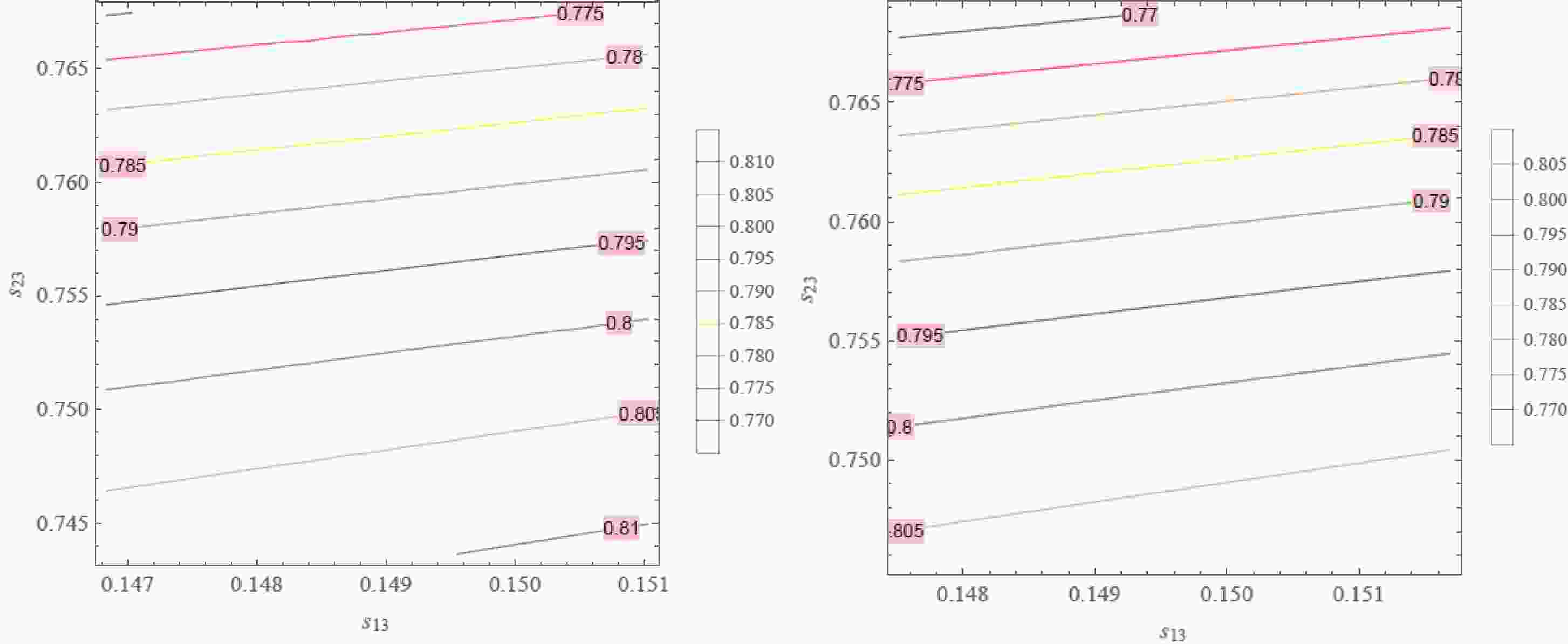
$ 1\, \sigma $ range④ [1],$ s_{13}\in (0.1468,\, 0.1510) $ and$ s_{23}\in (0.7436,\, 0.7675) $ for NH, while$ s_{13}\in (0.1475,\, 0.1517) $ and$ s_{23}\in (0.7457,\, 0.7688) $ for IH. Thus, from Eqs. (1) and (2) we can find the range of values of$ \cos\theta $ and$ \cos \alpha $ as plotted in Figs. 1, 2 and 3, respectively. On the other hand, since$ s^2_{13} $ is a very small and$ s^2_{23} $ is very close to$ \frac{1}{2} $ , we can assume$ {\cal{O}}(s^2_{13}, s^2_{23}) \ll 1 $ . Thus, from Eqs. (28) and (29) we can approximate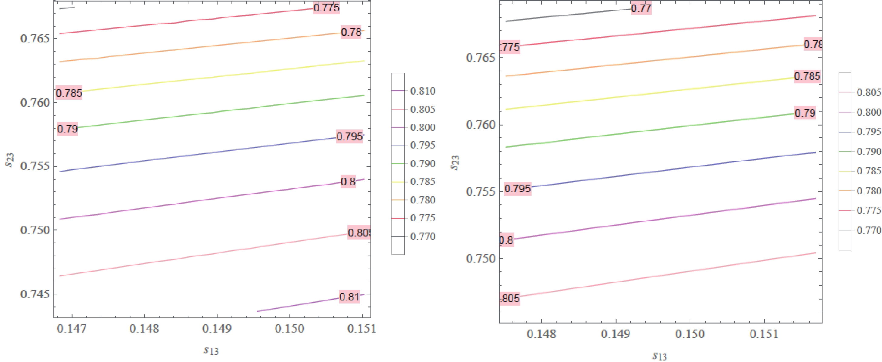
Figure 1. (color online) Contour plot of
$ \cos\theta $ as a function of$ s_{13} $ and$ s_{23} $ in the$ 1 \sigma $ range of the best-fit value taken from Ref. [1], i.e.$ s_{13}\in (0.1468,\, 0.1510) $ and$ s_{23}\in (0.7436,\, 0.7675) $ for NH (left), and$ s_{13}\in (0.1475,\, 0.1517) $ and$ s_{23}\in (0.7457,\, 0.7688) $ for IH (right).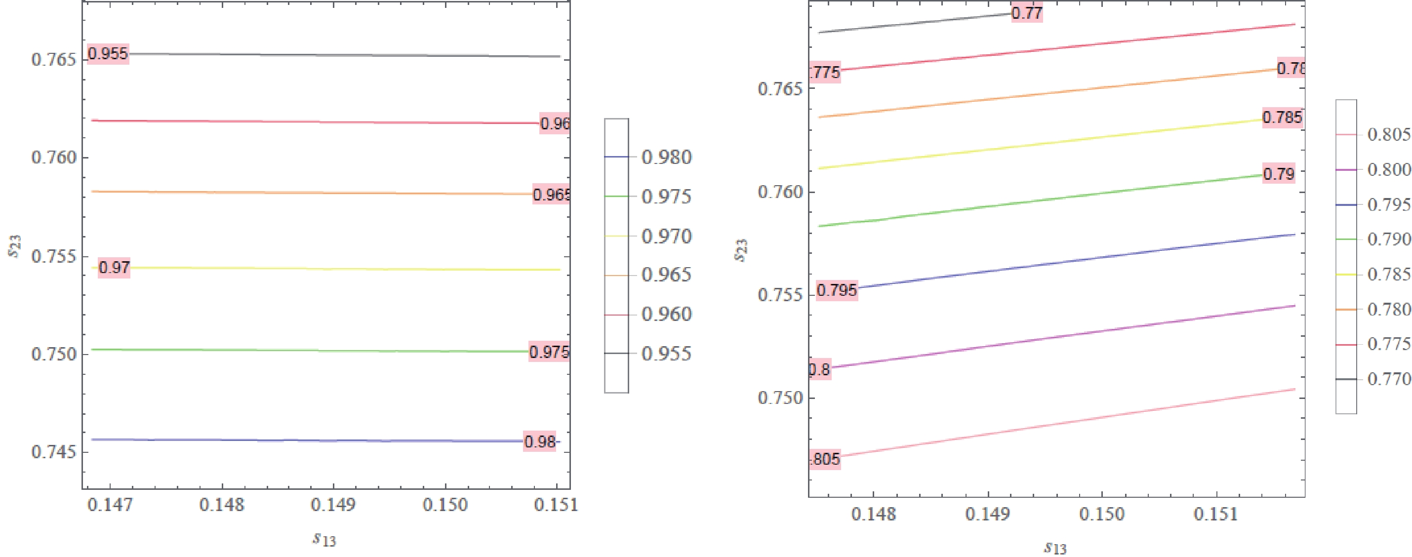
Figure 2. (color online) Contour plot of
$ \cos \alpha $ as a function of$ s_{13} $ and$ s_{23} $ in the$ 1 \sigma $ range of the best-fit value taken from Ref. [1], i.e.$ s_{13}\in (0.1468,\, 0.1510) $ and$ s_{23}\in (0.7436,\, 0.7675) $ for NH (left), and$ s_{13}\in (0.1475,\, 0.1517) $ and$ s_{23}\in (0.7457,\, 0.7688) $ for IH (right).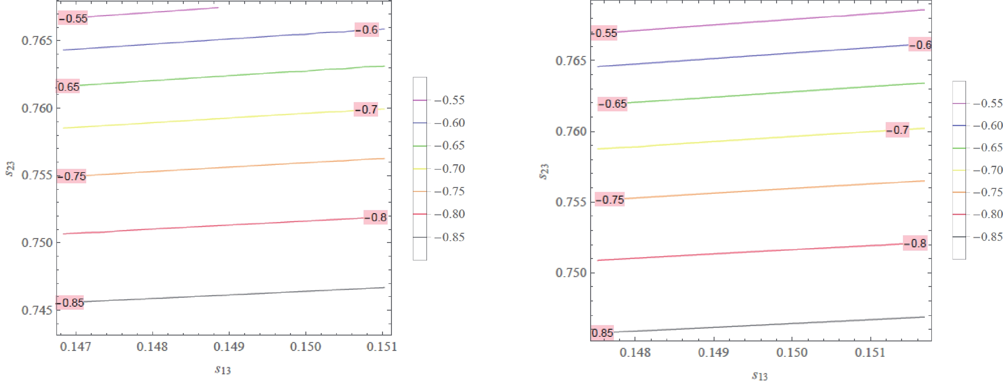
Figure 3. (color online) Contour plot of
$ \sin \delta $ as a function of$ s_{13} $ and$ s_{23} $ in the$ 1 \sigma $ range of the best-fit value taken from Ref. [1], i.e.$ s_{13}\in (0.1468,\, 0.1510) $ and$ s_{23}\in (0.7436,\, 0.7675) $ for NH (left ), and$ s_{13}\in (0.1475,\, 0.1517) $ and$ s_{23}\in (0.7457,\, 0.7688) $ for IH (right).$ \sin \delta \simeq -1 + \frac{{\cal{O}}(s^2_{13}, s^2_{23})}{8} <0. $

(33) Figure 3 shows that, in the
$ 1\, \sigma $ range of the best-fit value taken from Ref. [1], the range of the Dirac CP violating phase is defined as$ \sin \delta \in \left\{ \begin{array}{l} (-0.8664, -0.5688) \;\;{\rm{for}}\;\;{\rm{NH}}, \\ (-0.8509, -0.5462) \;\;{\rm{for}}\;\;{\rm{IH}}, \end{array} \right. $

(34) i.e.,
$ \delta \in \left\{ \begin{array}{l} (299.96,\, 325.33)^\circ \;\;{\rm{for}}\;\;{\rm{NH}}, \\ (301.70,\, 326.90)^\circ \;\;{\rm{for}}\;\;{\rm{IH}}. \end{array} \right. $

(35) In the case where
$ \theta_{23} $ takes its maximal values$ (\theta_{23} = \dfrac{\pi}{4}) $ ,$ {\cal{O}}(s^2_{13}, s^2_{23}) = 0 $ and$ \sin \delta = -1 $ , the model predicts the cobimaximal mixing pattern [58-69]:$ \theta_{13} \neq 0,\, \theta_{23} = \dfrac \pi 4 $ and$ \delta = - \dfrac \pi 2 $ . Furthermore, Eq. (30) implies$ t_{12}\in (0.7188,\, 0.7195) $ for NH and$ t_{12}\in (0.7189,\, 0.7196) $ for IH in the$ 1 \sigma $ range of$ s_{13} $ of the best-fit value taken from Ref. [1], which is plotted in Fig. 4. These intervals of$ \theta_{12} $ are in$ 3\, \sigma $ range of the best-fit value.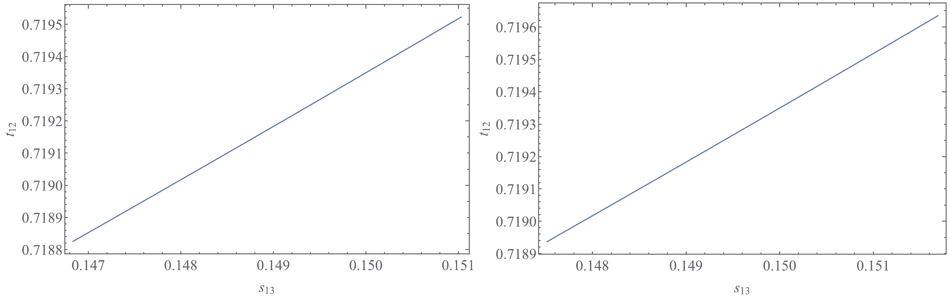
Figure 4. (color online)
$ t_{12} $ versus$ s_{13} $ with$ s_{13}\in (0.1468,\, 0.1510) $ for NH (left) and$ s_{13}\in (0.1475,\, 0.1517) $ for IH (right) for the$ 1 \sigma $ range of the best-fit value taken from Ref. [1].Figure 3 shows that, in our model,
$ \sin \delta \in (-0.851,\, -0.546) $ , i.e.$ \delta^\circ\in (300.0,\, 325) $ , for NH, and$ \sin\delta\in (-0.866,\, -0.569) $ , i.e.,$ \delta^\circ\in (301.679,\, 326.907) $ , for IH. Besides, in the$ 1 \sigma $ range [1],$ \delta^\circ_{\rm CP} \in (173,224) $ for NH and$ \delta^\circ_{\rm CP} \in (252,308) $ for IH, while in the$ 3 \sigma $ range [1],$ \delta^\circ_{\rm CP} \in (120,369) $ for NH and$ \delta^\circ_{\rm CP} \in (193,352) $ for IH. Hence, this model predicts the Dirac CP violating phase ($ \delta $ ) in which for NH,$ \delta $ is in$ 3\, \sigma $ range, and for IH,$ \delta $ is in$ 1\, \sigma $ range, of the best-fit values taken from Ref. [1].In order to fix the parameters, we should deal with the central values given in Table 1. For NH, taking the central values of
$ \theta_{23} $ and$ \theta_{13} $ as shown in Table 1,$ s_{23} = 0.757,\, s_{13} = 0.149 $ . For IH, taking the central values of$ \theta_{13} $ ,$ s_{13} = 0.1496 $ and$ s_{23} = 0.7517 $ , which are in the$ 1 \sigma $ range of the best-fit value taken from Ref. [1]. We get:$ \begin{array}{l} \theta = \left\{ \begin{array}{l} 37.47^\circ \;\;{\rm{for}}\;\;{\rm{NH}}, \\ 53.28^\circ\;\;{\rm{for}}\;\;{\rm{IH}}, \end{array} \right. \;\;\;\;\;\;\alpha = \left\{ \begin{array}{l} 14.84^\circ\;\;{\rm{for}}\;\;{\rm{NH}}, \\ 166.70^\circ\;\;{\rm{for}}\;\;{\rm{IH}} \end{array} \right. \quad \delta = \left\{ \begin{array}{l} 312.91^\circ \;\;{\rm{for}}\;\;{\rm{NH}}, \\ 307.03^\circ \;\;{\rm{for}}\;\;{\rm{IH}}, \end{array} \right.\;\;\;\; \theta_{12} = \left\{ \begin{array}{l} 35.72^\circ \;\;{\rm{for}}\;\;{\rm{NH}}, \\ 35.73^\circ\;\;{\rm{for}}\;\;{\rm{IH}}. \end{array} \right. \end{array} $

(36) Substituting Eq. (36) into Eq. (23) yields an explicit form of the leptonic mixing matrix:
${U_{\rm lep}} = \left\{ {\begin{array}{*{20}{l}} \begin{array}{l} \left( {\begin{array}{*{20}{c}} { 0.7977 - 0.08993{\rm i}}&{0.5774}&{0.1188 - 0.08993{\rm i}}\\ {0.3664 + 0.339{\rm i}}&{ - 0.2887 - 0.50{\rm i}}&{ - 0.5686 + 0.3069{\rm i}}\\ {{\mkern 1mu} 0.2106 - 0.2490{\rm i}}&{ - 0.2887 + 0.50{\rm i}}&{ - 0.5686 - 0.4868{\rm i}} \end{array}} \right)\;\;{\rm{for}}\;\;{\rm{NH}},\\ \left( {\begin{array}{*{20}{c}} { - 0.7956 + 0.1063{\rm i}}&{0.5774}&{ - 0.1053 - 0.1063{\rm i}}\\ { - 0.2779 - 0.1926{\rm i}}&{ - 0.2887 - 0.50{\rm i}}&{0.6624 - 0.3369{\rm i}}\\ { - 0.2779 + 0.4052{\rm i}}&{ - 0.2887 + 0.50{\rm i}}&{0.4783 + 0.4432{\rm i}} \end{array}} \right)\;\;{\mkern 1mu} {\rm{for}}\;\;{\rm{IH}}. \end{array} \end{array}} \right.$

(37) It has been checked that both forms of the leptonic mixing matrix
$ U_{\rm lep} $ given in Eq. (37) are unitary and consistent with the constraint given in Ref. [1].As a consequence, the Jarlskog invariant is given by
$ J_{\rm CP} = \left\{ \begin{array}{l} -2.501\times 10^{-2} \;\;{\rm{for}}\;\;{\rm{NH}}, \\ -2.744\times 10^{-2}\;\;{\rm{for}}\;\;{\rm{IH}}. \end{array} \right. $

(38) From the above analysis, we can conclude that the model under consideration can reproduce the recent experimental values of neutrino mixing angles and Dirac CP violating phase [1] in which the atmospheric angle
$ (\theta_{23}) $ and the reactor angle$ (\theta_{13}) $ get the best-fit values while the solar angle$ (\theta_{12}) $ and Dirac CP violating phase ($ \delta $ ) are in$ 3\, \sigma $ range of the best-fit value for the NH. For the IH,$ \theta_{13} $ has the best-fit value and$ \theta_{23} $ together with$ \delta $ are in the$ 1\, \sigma $ range, while$ \theta_{12} $ is in$ 3\, \sigma $ range of the best-fit value taken from Ref. [1]. Although the model results for$ t_{12} $ and$ \delta $ are in the$ 3\, \sigma $ range of the best-fit value from Ref. [1], they are within$ 2\, \sigma $ of the best-fit value taken from Ref. [70] and$ 1\, \sigma $ of the best-fit value taken from the SNO and KamLAND collaborations [71, 72]. Now we turn to the neutrino mass hierarchy. -
Taking into account the best-fit values of the neutrino mass-squared differences for NH given in Table 1,
$ \Delta m^2_{21} = 7.42 \times 10^{-5} {\rm{eV}}^2, \, \Delta m^2_{31} = 2.517\times 10^{-3}{\rm{eV}}^2 $ , we obtain a solution:$\begin{aligned}[b] \kappa _1 = \frac{\sum m_i}{2}- \frac{c_0}{2},\quad \kappa _2 = \frac{1}{2}\left(\sqrt{ \delta _{1N}}-\sqrt{ \delta _{2N}}\right), \end{aligned}$

(39) $ \begin{aligned}[b] c_0 =& \frac{\sum m_i}{3}-132.40 \delta _{1N}\sqrt{ \delta _{1N}}+2.102\\&\times 10^{-5}\left(\sqrt{ \delta _{1N}} +\sqrt{ \delta _{2N}}\right)\sqrt[3]{ \delta _{N}} \\ &+\sqrt{ \delta _{2N}}\Big[132.4 \delta _{2N}-0.3137\\&-264.90 \left(\sum m_i\right)^2\Big]+ \frac{\left(\sqrt{ \delta _{1N}} +\sqrt{ \delta _{2N}}\right) \delta _{3N}}{\sqrt[3]{ \delta _{N}}}, \end{aligned} $

(40) where
$ \delta _N $ and$ \delta _{iN} \, (i = 1-4) $ are given in Appendix A. Equations (17), (39), (40) and (A1)-(A5) show that the three neutrino masses$ m_{1,2,3} $ depend only on the sum of neutrino masses$ \sum_{i = 1}^3 m_i $ .At present there are various bounds on
$ \sum m_{i} $ . For instance, for the NH, the upper limit on the sum of neutrino masses is$ \sum m_i < 0.13\; {\rm{eV}} $ in the$ 2\, \sigma $ range [70]. The dependence of$ m_{1,2,3} $ on$ \sum m_i $ is plotted in Fig. 5 with$ \sum m_i \in \left(0.06, 0.1\right)\; {\rm{eV}} $ within$ 2\, \sigma $ range of the best-fit value taken from Ref. [70] and being well consistent with the strongest bound from cosmology [73]$ \sum m_\nu < 0.078 \; {\rm{eV}} $ ; the upper bounds are taken from Ref. [74]$ \sum m_\nu < 0.12 - 0.69 \; {\rm{eV}} $ , and the constraint in Ref. [75] is$ \sum m_\nu \in (0.06, 0.118)\; {\rm{eV}} $ . In the case$ \sum m_{i} = 6.5\times 10^{-2}\; {\rm{eV}} $ we get: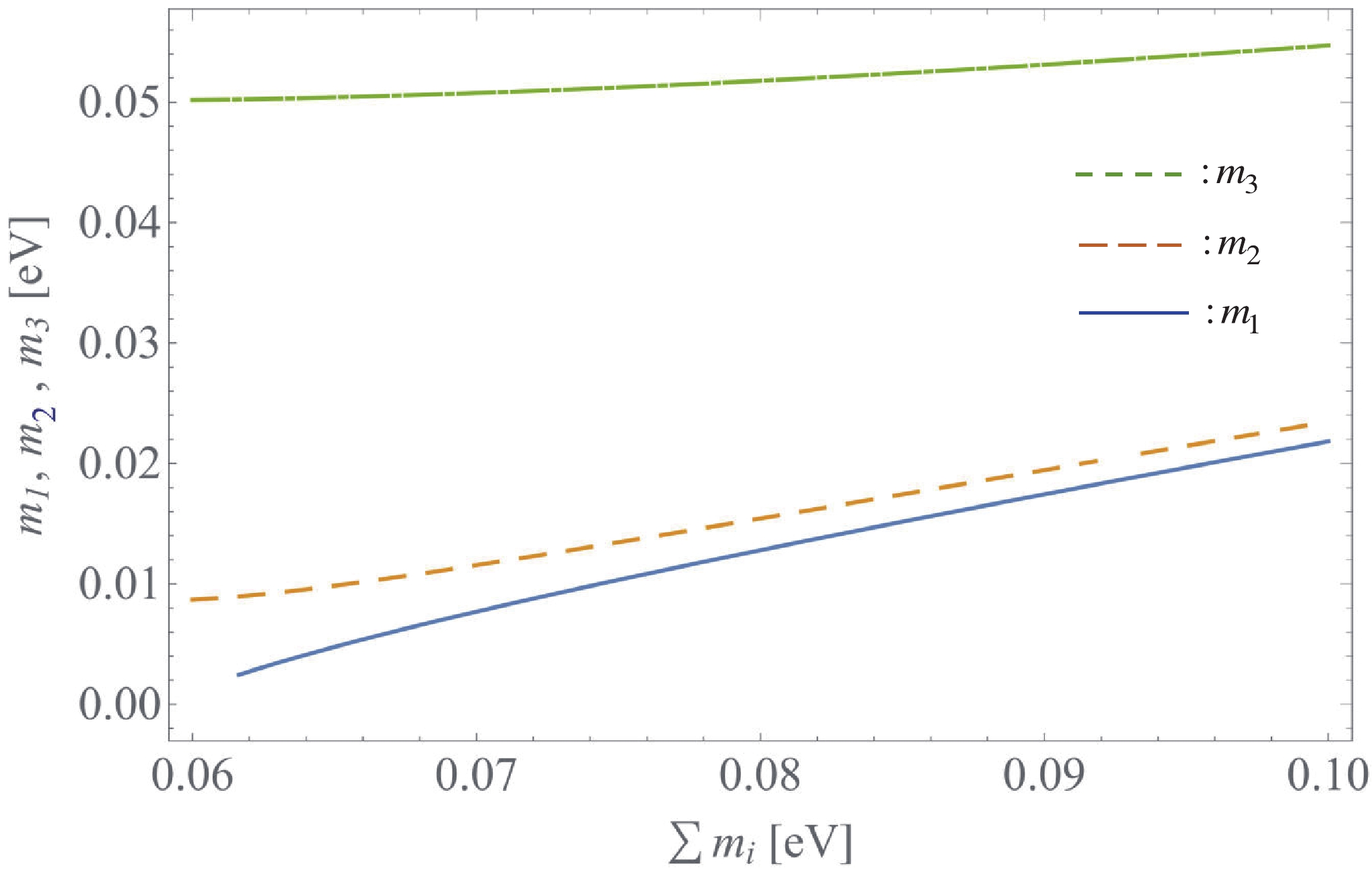
Figure 5. (color online)
$ m_{1,2,3} $ versus$ \sum m_i $ with$ \sum m_i \in \left(0.06, 0.1\right)\, {\rm{eV}} $ in the NH.$\begin{aligned}[b]& m_1 = 4.76\times 10^{-3}\, {\rm{eV}}, \\& m_2 = 9.84\times 10^{-3}\, {\rm{eV}}, \\&m_3 = 5.04\times 10^{-2}\, {\rm{eV}}. \end{aligned} $

(41) -
As before, using the best-fit values of the neutrino mass-squared differences for the IH shown in Table 1,
$ \Delta m^2_{21} = 7.42 \times 10^{-5} \;{\rm{eV}}^2,\, \Delta m^2_{32} = -2.498\times 10^{-3}\;{\rm{eV}}^2 $ , we get a solution:$ \begin{aligned}[b] & \kappa _1 = \frac{\sum m_i}{2}- \frac{c_0}{2}, \\& \kappa _2 = \frac{1}{2}\left(\sqrt{ \delta _{1I}}-\sqrt{ \delta _{2I}}\right), \end{aligned} $

(42) $ \begin{aligned}[b] c_0 =& \frac{\sum m_i}{3}-137.50 \delta _{1I}\sqrt{ \delta _{1I}}+2.183 \\&\times 10^{-5}\left(\sqrt{ \delta _{1I}} +\sqrt{ \delta _{2I}}\right)\sqrt[3]{ \delta _{I}} \\ &+\sqrt{ \delta _{2I}}\Big[137.50 \delta _{2I}+0.3537\\&-275.10 \left(\sum m_i\right)^2\Big]+ \frac{\left(\sqrt{ \delta _{1I}} +\sqrt{ \delta _{2I}}\right) \delta _{3I}}{\sqrt[3]{ \delta _{I}}}, \end{aligned} $

(43) where
$ \delta _I $ and$ \delta _{iI} \, (i = 1 - 4) $ are given in Appendix A. Similar to the previous section, the three neutrino masses$ m_{1,2,3} $ just depend on the sum of neutrino masses$ \sum_{i = 1}^3 m_i $ . For the IH, the tightest$ 2 \sigma $ upper limit on the sum of neutrino masses is$ \sum m_i < 0.15 \; {\rm{eV}} $ [70]. Furthermore, the upper bound taken from Ref. [74] is$ \sum m_\nu < 0.12 - 0.69\; {\rm{eV}} $ , while the constraint given in Ref. [75] is$ \sum m_\nu \in (0.1, 0.151)\; {\rm{eV}} $ . The dependence of the three active neutrino masses$ m_{1,2,3} $ on$ \sum m_i $ is plotted in Fig. 6 with$ \sum m_i \in \left(0.1, 0.2\right)\; {\rm{eV}} $ , which is well consistent with the recent constraints given in Refs. [70, 74, 75]. In the case$ \sum m_{i} = 0.1075\; {\rm{eV}} $ we get: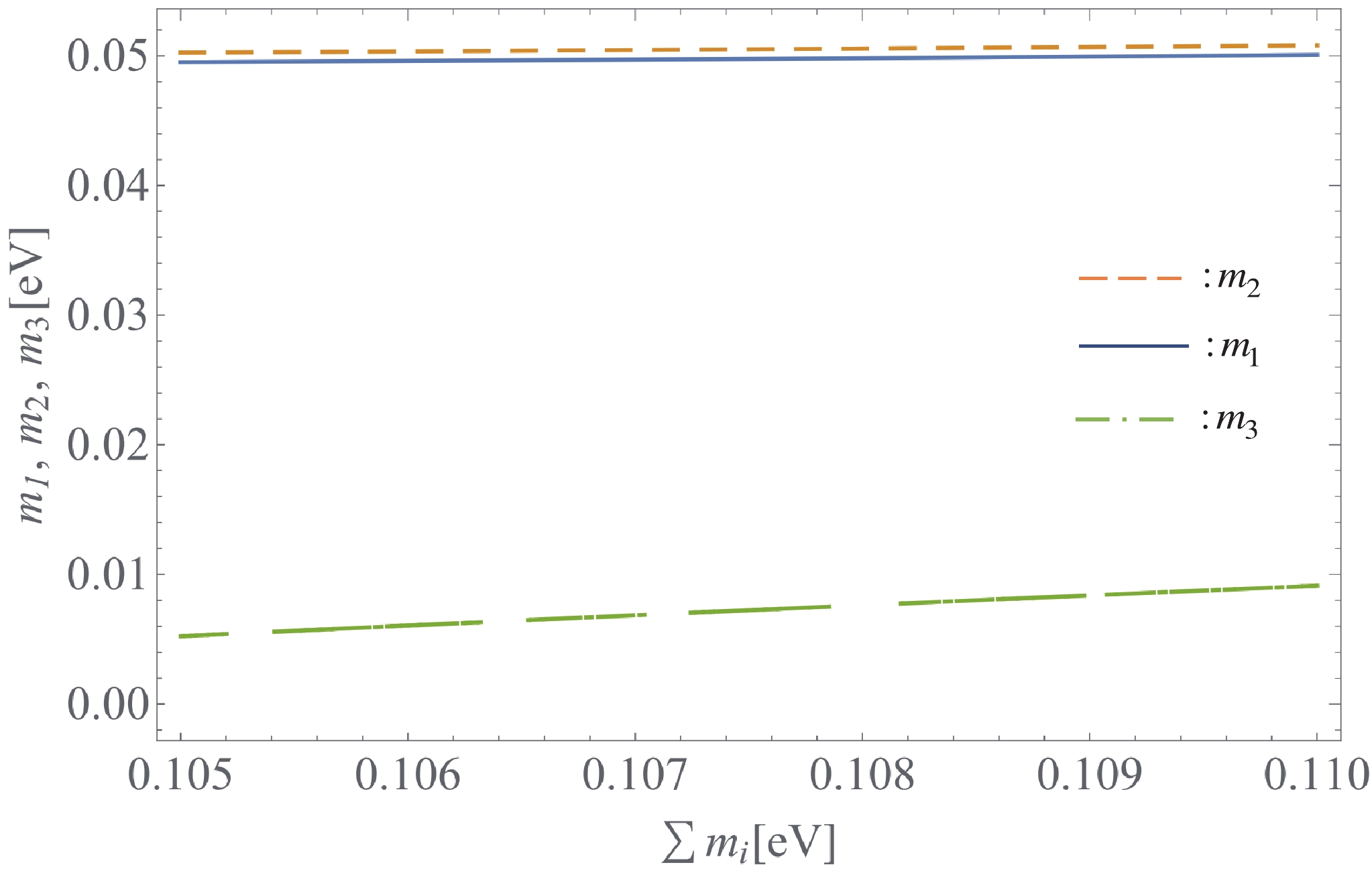
Figure 6. (color online)
$ m_{1,2,3} $ versus$ \sum m_i $ with$ \sum m_i \in \left(0.105, 0.11\right)\, {\rm{eV}} $ in the IH.$\begin{aligned}[b]& m_1 = 4.976\times 10^{-2}\; {\rm{eV}},\\ & m_2 = 5.05\times 10^{-2}\; {\rm{eV}}, \\ &m_3 = 7.237\times 10^{-3}\; {\rm{eV}}. \end{aligned}$

(44) -
Now, we deal with an effective neutrino mass. Equations (17), (39), (40) and (A1)-(A5) (for NH) and (17), (42), (43) and (A6)-(A10) (for IH) show that, with the best-fit values of the neutrino mass-squared differences, the effective neutrino mass parameters
$ \langle m_{ee}\rangle $ and$ m_\beta $ depend on the sum of neutrino masses$ \sum_{i = 1}^3 m_i $ and two mixing angles$ \theta_{23},\, \theta_{13} $ . In the NH,$ m_1< m_2<m_3 $ , hence$ m_1\equiv m_{\rm light} $ is the lightest neutrino mass, while in the IH,$ m_3< m_1< m_2 $ , therefore$ m_3\equiv m_{\rm light} $ is the lightest neutrino mass. If we fix$ \theta_{23} $ and$ \theta_{13} $ at their best-fit values taken in Table 1, the effective neutrino masses$ \langle m_{ee}\rangle, \;m_{\beta} $ and$ m_{\rm light} $ as functions of$ \sum m_i $ are as plotted in Fig. 7.
Figure 7. (color online)
$ \langle m_{ee} \rangle,\; m_\beta $ and$ m_{\rm light} $ versus$ \sum m_i $ with$ \sum m_i \in \left(0.06, \;0.1\right)\, {\rm{eV}} $ in the NH (left) and$ \sum m_i \in \left(0.105, \;0.11\right)\; {\rm{eV}} $ in the IH (right).In order to see the dependence of
$ \langle m_{ee} \rangle $ and$ m_\beta $ on$ \theta_{23} $ and$ \theta_{13} $ we can fix the value for$ \sum m_i $ in its constraint range [70, 74]. For instance,$ \sum m_i = 0.065\; {\rm{eV}} $ for NH and$ \sum m_i = 0.1075\, {\rm{eV}} $ for IH. Consequently, we can contour plot$ \langle m_{ee} \rangle $ and$ m_\beta $ as functions of ($ \theta_{23},\,\theta_{13} $ ), as shown in Figs. 8 and 9, respectively.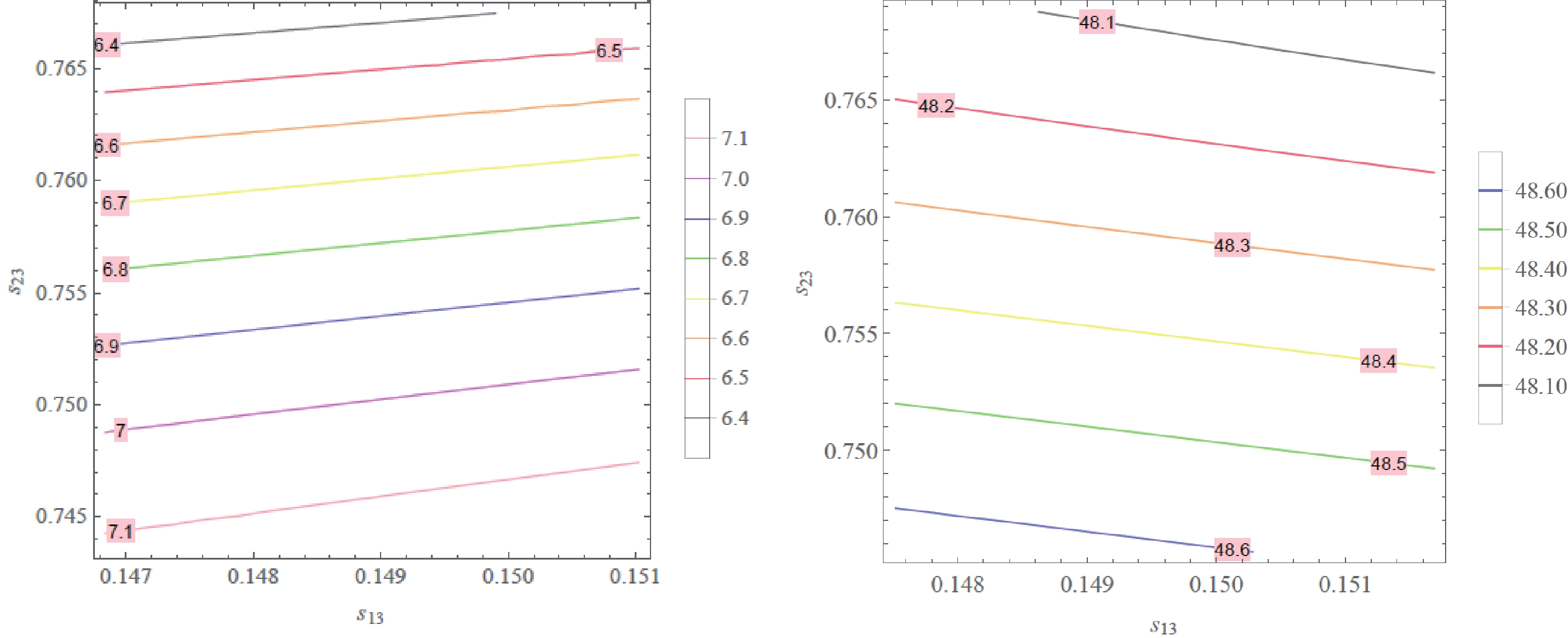
Figure 8. (color online) Contour plot of
$ \langle m_{ee}\rangle \, ({\rm{meV}}) $ as a function of$ s_{13} $ and$ s_{23} $ in the$ 1 \sigma $ range of the best-fit values:$ s_{13}\in (0.1468,\, 0.1510) $ and$ s_{23}\in (0.7436,\, 0.7675) $ for NH (left), and$ s_{13}\in (0.1475,\, 0.1517) $ and$ s_{23}\in (0.7457,\, 0.7688) $ for IH (right).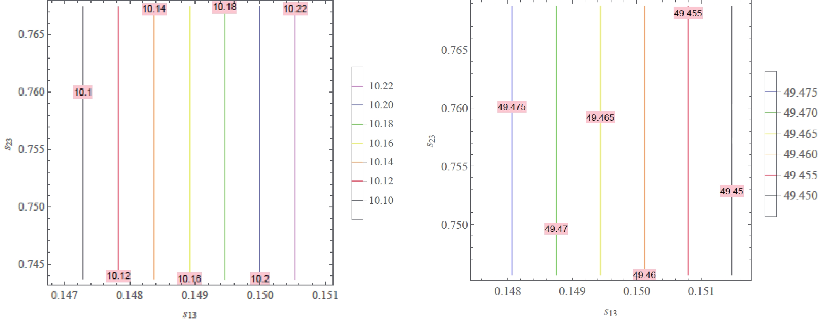
Figure 9. (color online) Contour plot of
$ m_\beta \, ({\rm{meV}}) $ as a function of$ s_{13} $ and$ s_{23} $ in the$ 1 \sigma $ range of the best-fit values:$ s_{13}\in (0.1468,\, 0.1510) $ and$ s_{23}\in (0.7436,\, 0.7675) $ for NH (left), and$ s_{13}\in (0.1475,\, 0.1517) $ and$ s_{23}\in (0.7457,\, 0.7688) $ for IH (right).These figures show that at
$ 1\, \sigma $ range of the best-fit value taken from Ref. [1] of$ s_{23} $ and$ s_{13} $ , the model predicts the range of the effective neutrino mass parameters as follows:$ \langle m_{ee}\rangle \in\left\{ \begin{array}{l} (6.40,\,\, 7.10) \,\, {\rm{meV}}\ \ \ \ \ {\rm{for}} \ \ {\rm{NH}}, \\ (48.04,\, 48.64)\,\, {\rm{meV}}\ \ {\rm{for}} \ \ \ {\rm{IH}}, \end{array} \right. $

(45) and
$ m_{\beta}\in\left\{ \begin{array}{l} (10.10,\,\, 10.22) \,\, {\rm{meV}}\ \ \ \ \ \ {\rm{for}} \ \ \ \ {\rm{NH}}, \\ (49.45,\,49.48)\,\, {\rm{meV}}\ \ \ \ {\rm{for}} \ \ \ \ {\rm{IH}}. \end{array} \right. $

(46) In the case where
$ s_{23} $ and$ s_{13} $ take their best-fit values [1],$ s_{23} = 0.757,\, s_{13} = 0.149 $ for NH and for$ s_{23} = 0.7583, \, s_{13} = 0.1496 $ IH, one gets:$ \langle m_{ee}\rangle = \left\{ \begin{array}{l} 6.81 \,\, {\rm{meV}}\ \ \ \ \ {\rm{for}} \ \ \ \ {\rm{NH}}, \\ 48.48 \,\, {\rm{meV}}\ \ \ \ {\rm{for}} \ \ \ \ {\rm{IH}}, \end{array} \right. $

(47) and
$ m_{\beta} = \left\{ \begin{array}{l} 10.20 \,\, {\rm{meV}}\ \ \ \ \ {\rm{for}} \ \ \ \ {\rm{NH}}, \\ 49.46\,\, {\rm{meV}}\ \ \ \ {\rm{for}} \ \ \ \ {\rm{IH}}. \end{array} \right. $

(48) The derived effective neutrino mass parameters in Eqs. (47) and (48) satisfy all the upper bounds arising from recent
$ 0\nu \beta \beta $ decay experiments taken from KamLAND-Zen [76]$ \langle m_{ee} \rangle <61 - 165 \;{\rm{meV}} $ , GERDA [77]$ \langle m_{ee} \rangle < 104 - 228 \;{\rm{meV}} $ and CUORE [78]$ \langle m_{ee} \rangle < 75 - 350 \;{\rm{meV}} $ . -
We have suggested a multiscalar and nonrenormalizable
$ U(1)_{B-L} $ extension of the SM with$ S_4 $ symmetry which successfully explains the recent observed neutrino oscillation data. The tiny neutrino mass and the neutrino mass hierarchies are generated via the type-I seesaw mechanism. The model reproduces the recent experimental data of neutrino mixing angles and Dirac CP violating phase in which the atmospheric angle$ (\theta_{23}) $ and the reactor angle$ (\theta_{13}) $ get the best-fit values while the solar angle$ (\theta_{12}) $ and Dirac CP violating phase ($ \delta $ ) are in$ 3\, \sigma $ range of the best-fit value for the NH. For the IH,$ \theta_{13} $ gets the best-fit value and$ \theta_{23} $ together with$ \delta $ are in the$ 1\, \sigma $ range, while$ \theta_{12} $ belongs to$ 3\, \sigma $ range of the best-fit value. The effective neutrino masses are predicted to be$ \langle m_{ee}\rangle = 6.81 \; {\rm{meV}} $ for the NH and$ \langle m_{ee}\rangle = 48.48\;{\rm{meV}} $ for the IH, while$ m_{\beta} = 10.20\; {\rm{meV}} $ for the NH and$ m_{\beta} = 49.46\;{\rm{meV}} $ for the IH, which are strongly consistent with the most recent experimental data. -
The parameters
$ \delta _{N(I)} $ and$ \delta _{iN(I)} \, (i = 1 - 4) $ in Eqs. (39), (40), (42), (43) have explicit expressions as follows:$\tag{A1} \begin{aligned}[b] \delta _{1N} =& 7.895\times 10^{-4}+5.291\times 10^{-8}\sqrt[3]{ \delta _{N}}+ \frac{2}{3}\left(\sum m_i\right)^2 \\ &- \frac{26.99-4979\left(\sum m_i\right)^2-2.10\times 10^6 \left(\sum m_i\right)^4}{\sqrt[3]{ \delta _{N}}}, \end{aligned} $

$\tag{A2} \begin{aligned}[b] \delta _{2N} =& 1.5795\times 10^{-3}+5.291\times 10^{-8}\sqrt[3]{ \delta _{N}}+ \frac{4}{3}\left(\sum m_i\right)^2 \\ &+ \frac{26.99-4979\left(\sum m_i\right)^2-2.10\times 10^6 \left(\sum m_i\right)^4}{\sqrt[3]{ \delta _{N}}}\\&+ \frac{5.034\times 10^{-3} \sum m_i}{\sqrt{ \delta _{1N}}}, \end{aligned} $

$\tag{A3} \begin{aligned}[b] \delta _{3N} =& -1.0722\times 10^4 + 1.976\times 10^6 \left(\sum m_i\right)^2 \\&+ 8.343\times 10^8 \left(\sum m_i\right)^4, \end{aligned} $

$\tag{A4} \begin{aligned}[b] \delta _{N} =& -1.308\times 10^{13}+9.639\times 10^{15}\left(\sum m_i\right)^2 \\&-8.882\times 10^{17}\left(\sum m_i\right)^4 \\&- 2.50\times 10^{20}\left(\sum m_i\right)^6 -6.539\times 10^{12}\sqrt{ \delta _{4N}}, \end{aligned} $

$\tag{A5} \begin{aligned}[b] \delta _{4N} = &7.101-7.61 \times 10^3\left(\sum m_i\right)^2\\&+2.308\times 10^6\left(\sum m_i\right)^4-6.65\times 10^{10}\left(\sum m_i\right)^{8}. \end{aligned}$

$\tag{A6} \begin{aligned}[b] \delta _{1I} =& -8.574\times 10^{-4}+5.291\times 10^{-8}\sqrt[3]{ \delta _{I}}+ \frac{2}{3}\left(\sum m_i\right)^2 \\ &- \frac{24.28+5401\left(\sum m_i\right)^2-2.10\times 10^6 \left(\sum m_i\right)^4}{\sqrt[3]{ \delta _{I}}}, \end{aligned} $

$\tag{A7} \begin{aligned}[b] \delta _{2I} =& -1.715\times 10^{-3}-5.291\times 10^{-8}\sqrt[3]{ \delta _{I}}+ \frac{4}{3}\left(\sum m_i\right)^2 \\&+ \frac{24.28+5401\left(\sum m_i\right)^2-2.10\times 10^6 \left(\sum m_i\right)^4}{\sqrt[3]{ \delta _{I}}}\\&- \frac{4.848\times 10^{-3} \sum m_i}{\sqrt{ \delta _{1I}}}, \end{aligned} $

$\tag{A8}\begin{aligned}[b] \delta _{3I} =& -1.002\times 10^4 -2.228\times 10^6 \left(\sum m_i\right)^2 \\&+ 8.664\times 10^8 \left(\sum m_i\right)^4, \end{aligned} $

$\tag{A9} \begin{aligned}[b] \delta _{I} =& 1.328\times 10^{13}+8.673\times 10^{15}\left(\sum m_i\right)^2 \\&+9.646\times 10^{17}\left(\sum m_i\right)^4 \\&-2.50\times 10^{20}\left(\sum m_i\right)^6 -6.297\times 10^{12}\sqrt{ \delta _{4I}}, \end{aligned} $

$ \tag{A10}\begin{aligned}[b] \delta _{4I} =& 6.886+7.436\times 10^3\left(\sum m_i\right)^2\\&+2.273\times 10^6\left(\sum m_i\right)^4-6.25\times 10^{10}\left(\sum m_i\right)^{8}. \,\, \end{aligned} $

Multiscalar B-L extension based on S4 flavor symmetry for neutrino masses and mixing
- Received Date: 2020-12-08
- Available Online: 2021-04-15
Abstract: A multiscalar and nonrenormalizable


 DownLoad: