Measurements of decay branching fractions of the Higgs boson to hadronic final states at the CEPC

The discovery of the Higgs boson by the ATLAS and CMS collaborations at the Large Hadron Collider (LHC) in July 2012 [1, 2] marked a significant breakthrough in particle physics, providing deeper insights into the Standard Model (SM). While the SM has been successful in describing the fundamental building blocks of matter and their interactions, several unanswered questions remain, such as the origin of dark matter and the inability to unify all fundamental forces. As a promising gateway to new physics, precise measurements of the Higgs boson’s properties are essential for testing the SM and uncovering potential hints of physics beyond the Standard Model (BSM).

In comparison with the LHC, which relies on high-energy proton-proton ($ pp $) collisions, a lepton collider offers more energy control and significantly lowers pileup contamination (average number of$ pp $interactions per beam crossing), serving as a Higgs factory. Several lepton colliders have been proposed for reconfirming the discovery of a Higgs-like particle and studying the properties of the Higgs boson with high precision, including CLIC [3], FCC-ee [4], and ILC [5]. Among the aforementioned colliders, the Circular Electron Positron Collider (CEPC) [6, 7] was proposed by the Chinese High Energy Physics Community in 2012. It is designed to operate at a center-of-mass energy of 240 GeV to 250 GeV with an integrated luminosity of 5600 fb⁻¹. The main Higgs production process in CEPC will be via associated production with a Z boson, $ e^{+}e^{-} \to ZH $, where the Z boson is expected to undergo further decay.

According to theoretical predictions, the branching fractions of the decay of a 125 GeV Higgs boson into $ b\overline{b} $, $ c\overline{c} $, $ gg $, $ \tau\overline{\tau} $, $ WW^{*} $, and$ ZZ^{*} $ are 57.7%, 2.91%, 8.57%, 6.32%, 21.5% and 2.64%, respectively [8−10]. The Higgs boson decay into $ b\overline{b} $, $ WW^{*} $, and$ ZZ^{*} $ was studied by the ATLAS Collaboration using a 13 TeV $ pp $ Run 2 dataset collected at a center-of-mass energy of 13 TeV with a luminosity of 139 fb⁻¹ at the LHC. The branching fractions were measured to be $ 0.53\pm0.08 $, $ 0.257^{+0.026}_{-0.024} $, and 0.028$ \pm $ 0.003, respectively [11].

The work presented here focuses on the determination of the branching fractions of the Higgs boson decaying into a pair of b-quarks or c-quarks, gluons, $ \tau\overline{\tau} $, $ WW^{*} $, or $ ZZ^{*} $ in associated $ Z(\mu^+\mu^-)H $ production, where the W or Z bosons decay hadronically, at the CEPC with a center-of-mass energy of 240 GeV and integrated luminosity of 5600 fb⁻¹. The branching fraction measurements for $ H\to b\overline{b} /c\overline{c} /gg/\tau\overline{\tau}/WW^{*} /ZZ^{*} $ will be conducted simultaneously considering the major background sources. Since the dominant decay modes of $ WW^{*} $ and $ ZZ^{*} $ are hadronic, all the six processes primarily produce final states with jets, making it challenging to distinguish them. This difficulty can be overcome by employing the Particle Flow Network (PFN) [12], which is used for jet tagging, due to its ability to distinguish these processes. In contrast with traditional jet tagging methods based on QCD theory, which measure branching fractions channel by channel, PFN separates all channels in a single implementation with high accuracy.

This paper is organized as follows: Section II provides a brief description of the collider and Monte Carlo (MC) simulations. Event selection requirements are detailed in Section III. Section IV discusses the modeling using PFNs, with their performance evaluated in Section V. The procedure for determining the branching fractions is explained in Section VI, followed by the results in Section VII, where the measurements and their associated statistical and systematic uncertainties are discussed. A brief summary of the study is given in Section VIII.

The CEPC is a circular electron positron collider with a total circumference of 100 km. Its center of mass energy could reach the Z pole (91.2 GeV), the $ WW $ threshold (161 GeV), and the Higgs factory (240 GeV). The CEPC detector employs a highly granular calorimetry system to separate the particle showers, and a low material tracking system to minimize the interaction of the final state particles in the tracking material. It contains a vertex detector with a high spatial resolution, a Time Projection Chamber (TPC), a silicon tracker, a silicon-tungsten sampling Electromagnetic Calorimeter (ECAL), and a steel-Glass Resistive Plate Chambers (GRPC) sampling Hadronic Calorimeter (HCAL). The CEPC detector magnet is an iron-yoke-based solenoid that provides an axial magnetic field of 3 T at the interaction point. The outermost part of the detector is a flux return yoke embedded with a muon detector, which identifies muons inside jets. Further details can be found in Ref. [7].

The signal and background events are both generated using the MC generator Whizard 1.95 [13] and Pythia6 [14] for fragmentation and hadronization. The response of the CEPC detector is simulated using a Delphes-based software suite for fast detector simulation [15] according to the performance of the baseline detector in the CEPC CDR [7]. The resolution of the impact parameter in the $ r\phi $plane is obtained as

The resolution of particle transverse momenta is

The energy resolution of photons is

and that of neutral hadrons is:

In this analysis, Higgs production via the$ ZH $ process is considered to be the dominant process with Z decaying to a pair of muons and Higgs boson decaying in pairs of $ b\overline{b} /c\overline{c} /gg/\tau\overline{\tau}/WW^{*} /ZZ^{*} $ is the signal process. Additionally, the inclusive decays of $ H\to WW^{*} $ and $ H\to ZZ^{*} $ are considered. The backgrounds originate from processes with two-fermion and four-fermion final states. The two-fermion background processes include $ l\bar{l} $, $ \nu\bar{\nu} $, and $ q\bar{q} $, referring to final states with leptons (l), neutrinos (ν), and quarks (q). The four-fermion background includes $ (ZZ)_h $, $ (ZZ)_l $, $ (ZZ)_{sl} $, $ (WW)_h $, $ (WW)_l $, $ (WW)_{sl} $, $ (SZ)_l $, $ (SZ)_{sl} $, $ (SW)_l $, $ (SW)_{sl} $, $ (mix)_h $, and $ (mix)_{l} $, referring to final states with leptons (l), hadrons (h), and semi-leptons (sl). Table 1 presents the cross sections of the signal processes. Table 2 provides a summary of the detailed decay modes of the two-fermion and four-fermion backgrounds along with their cross sections.

Process	Higgs decays	Cross section/fb
$ ZH $ process	$ H\to b\overline{b} $	3.91
	$ H\to c\overline{c} $	0.20
	$ H\to gg $	0.58
	$ H\to \tau\overline{\tau} $	0.42
	$ H\to WW^{*} $	1.46
	$ H\to ZZ^{*} $	0.18

Table 1.  Cross sections for the Higgs production via the$ ZH $ process, where Z boson decays to a muon pair and the Higgs boson decays to $ b\overline{b} /c\overline{c} /gg $ and $ \tau\overline{\tau}/WW^{*} /ZZ^{*} $, with the W or Z bosons decaying hadronically.

Category	Name	Decay modes	Cross section/fb
Two-fermion background	$ l\bar{l} $	$ e^{+}e^{-} \to e^{+}e^{-} $	24770.90
		$ e^{+}e^{-} \to \mu^{+}\mu^{-} $	5332.71
		$ e^{+}e^{-}\to\tau^{+}\tau^{-} $	4752.89
	$ \nu\bar{\nu} $	$ e^{+}e^{-} \to \nu_{e}\bar{\nu}_{e} $	45390.79
		$ e^{+}e^{-} \to \nu_{\mu}\bar{\nu}_{\mu} $	4416.30
		$ e^{+}e^{-}\to \nu_{\tau}\bar{\nu}_{\tau} $	4410.26
	$ q\bar{q} $	$ e^{+}e^{-} \to u\bar{u} $	10899.33
		$ e^{+}e^{-} \to d\bar{d} $	10711.01
		$ e^{+}e^{-}\to c\bar{c} $	10862.86
		$ e^{+}e^{-} \to s\bar{s} $	10737.84
		$ e^{+}e^{-} \to b\bar{b} $	10769.78
Four-fermion background	$ (ZZ)_h $	$ Z \to c\bar{c},Z \to d\bar{d}/b\bar{b} $	98.97
		$ ZZ \to d\bar{d}d\bar{d} $	233.46
		$ ZZ \to u\bar{u}u\bar{u} $	85.68
		$ Z \to u\bar{u},Z \to s\bar{s}/b\bar{b} $	98.56
	$ (ZZ)_l $	$ Z\to\mu^{+}\mu^{-},Z\to\mu^{+}\mu^{-} $	15.56
		$ Z\to\tau^{+}\tau^{-},Z\to\tau^{+}\tau^{-} $	4.61
		$ Z\to\mu^{+}\mu^{-},Z\to\nu_{\mu}\bar{\nu}_{\mu} $	19.38
		$ Z\to\tau^{+}\tau^{-},Z\to\mu^{+}\mu^{-} $	18.65
		$ Z\to\tau^{+}\tau^{-},Z\to\nu_{\tau}\bar{\nu}_{\tau} $	9.61
	$ (ZZ)_{sl} $	$ Z\to\mu^{+}\mu^{-},Z\to d\bar{d} $	136.14
		$ Z\to\mu^{+}\mu^{-},Z\to u\bar{u} $	87.39
		$ Z\to\nu\bar{\nu},Z\to d\bar{d} $	139.71
		$ Z\to\nu\bar{\nu},Z\to u\bar{u} $	84.38
		$ Z\to\tau^{+}\tau^{-},Z\to d\bar{d} $	67.31
		$ Z\to\tau^{+}\tau^{-},Z\to u\bar{u} $	41.56
	$ (WW)_{h} $	$ WW\to uubd $	0.05
		$ WW\to ccbs $	5.89
		$ WW\to ccds $	170.18
		$ WW\to cusd $	3478.89
		$ WW\to uusd $	170.45
Continued on next page

Table 2.  Detailed decay modes for two-fermion ($l\bar{l}$, $\nu\bar{\nu}$ and $q\bar{q}$) and four-fermion ($(ZZ)_h$, $(ZZ)_l$, $(ZZ)_{sl}$, $(WW)_h$, $(WW)_l$, $(WW)_{sl}$, $(SZ)_l$, $(SZ)_{sl}$, $(SW)_l$, $(SW)_{sl}$, $(mix)_h$ and $(mix)_{l}$) backgrounds and their cross sections.

Table 2-continued from previous page
Category	Name	Decay modes	Cross section/fb
Four-fermion background	$ (WW)_{l} $	$ WW\to 4leptons $	403.66
	$ (WW)_{sl} $	$ W\to\mu\bar{\nu}_{\mu},W\to q\bar{q} $	2423.43
		$ W\to\tau\bar{\nu}_{\tau},W\to q\bar{q} $	2423.56
	$ (SZ)_{l} $	$ e^{+}e^{-},Z\to e^{+}e^{-} $	78.49
		$ e^{+}e^{-},Z\to \mu^{+}\mu^{-} $	845.81
		$ e^{+}e^{-},Z\to \nu\nu $	28.94
		$ e^{+}e^{-},Z\to \tau^{+}\tau^{-} $	147.28
		$ \nu^{+}\nu^{-},Z\to \mu^{+}\mu^{-} $	43.42
		$ \nu^{+}\nu^{-},Z\to \tau^{+}\tau^{-} $	14.57
	$ (SZ)_{sl} $	$ e^{+}e^{-},Z\to d\bar{d} $	125.83
		$ e^{+}e^{-}, Z\to u\bar{u} $	190.21
		$ \nu^{+}\nu^{-},Z\to d\bar{d} $	90.03
		$ \nu^{+}\nu^{-},Z\to u\bar{u} $	55.59
	$ (SW)_{l} $	$ e\nu_{e},W\to \mu\nu_{\mu} $	436.70
		$ e\nu_{e},W\to \tau\nu_{\tau} $	435.93
	$ (SW)_{sl} $	$ e\nu_{e},W\to qq $	2612.62
	$ (mix)_{h} $	$ ZZ/WW\to ccss $	1607.55
		$ ZZ/WW\to uudd $	1610.32
	$ (mix)_{l} $	$ ZZ/WW\to \mu\mu\nu_{\mu}\nu_{\mu} $	221.10
		$ ZZ/WW\to\tau\tau\nu_{\tau}\nu_{\tau} $	211.18
		$ SZ/SW\to ee\nu_{e}\nu_{e} $	249.48

The following criteria are applied to select events for further analysis. Each event must contain at least two tracks with opposite charges reconstructed as a muon pair ($ \mu^{+}\mu^{-} $). The muon candidates in each event must be isolated by satisfying $ E_{\text{cone}}^{2} <4E_{\mu } +12.2 $GeV [16], where $ E_{\text{cone}} $ is the sum of energy within a cone ($ \cos\theta _{\text{cone}} > 0.98 $) around the muon. When more than two muons are selected, the muon pair with an invariant mass closest to the Z boson mass, corresponding to a Z-mass window of 75 GeV to 105 GeV, is chosen as the Z candidate. The invariant mass of the recoil system, $ M_{\mu\mu}^{\text{recoil}} $, against the Z boson candidate is defined as

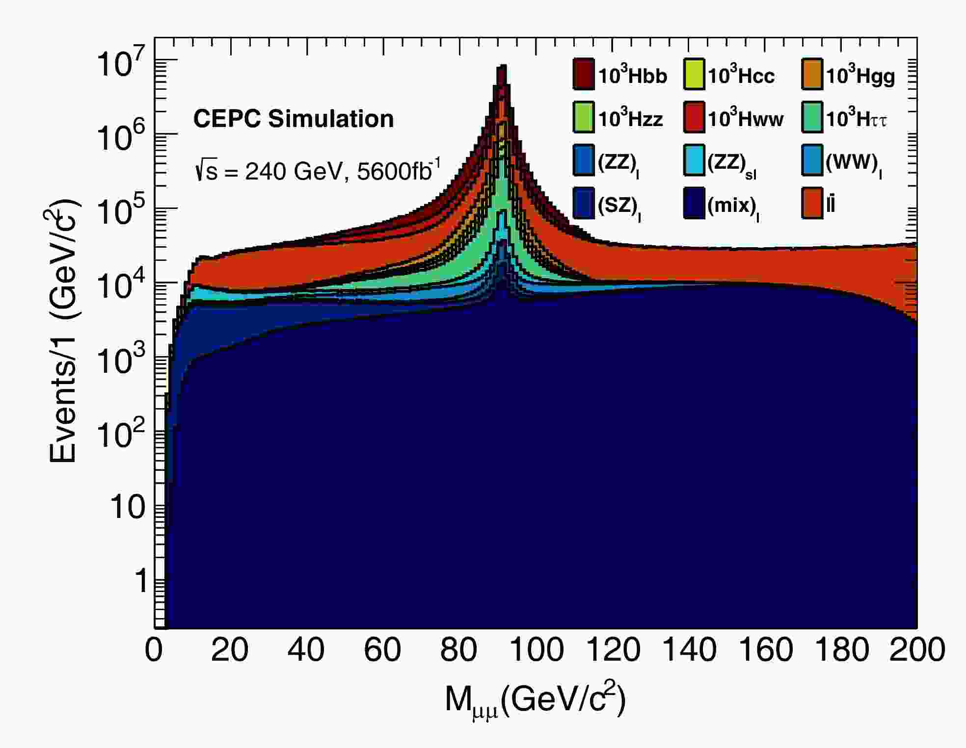
where $ \sqrt{s} = 240 $ GeV, while E and $ \overrightarrow{P} $ represent the energy and momentum of the muons, respectively. Using this equation, $ M_{\mu\mu}^{\text{recoil}} $ must fall within the Higgs mass window of 110 GeV to 150 GeV. To further reduce the two-fermion background, the polar angle of the muon pair system must be in the range of $ |\cos\theta_{\mu^{+}\mu^{-}}|<0.996 $.

Figure 1 shows the invariant mass distribution of the selected muon pair, and Fig. 2 presents the invariant mass distribution of the muon pair recoil system for both signal and background events after the isolation and muon pair criteria have been applied. In both distributions, a high signal efficiency of more than 90% is achieved, while the background contributions are significantly suppressed by the applied mass window selections.

Figure 1.  (color online) Invariant mass distributions of the muon pair for signal and background events after applying the muon pair and isolation selection criteria. The signal is well preserved, maintaining a high efficiency exceeding 90%, while background contributions are largely suppressed. Signal events are normalized to 1000 times the expected yields, and background events are normalized to their expected yields in data with an integrated luminosity of 5600 fb⁻¹.

Figure 2.  (color online) Invariant mass distributions of the muon pair recoil system for signal and background events after applying muon pair and isolation selection criteria. The signal is well preserved, retaining an efficiency of over 90%, while background contributions are significantly suppressed. Signal events are normalized to 1000 times the expected yields, and background events are normalized to their expected yields in data with an integrated luminosity of 5600 fb⁻¹.

Table 3 presents the event selection efficiencies for various signal and background processes, detailing the efficiency at each selection step relative to the previous requirement. In addition, the total efficiency is defined as the ratio of the number of events satisfying all selection criteria to the total number of events expected from the considered process (signal or background). For signal processes, a high efficiency of over 80% is observed. In contrast, two-fermion background processes, primarily $ l\bar{l} $, exhibit a total efficiency of around 0.3% and other contributions are negligible. Four-fermion backgrounds, such as $ (ZZ)_l $, $ (ZZ)_{sl} $, and $ (WW)_l $, have total efficiencies of 3.3%, 1.3%, and 2.1%, respectively, while $ (ZZ)_h $, $ (WW)_{h} $, and $ (WW)_{sl} $ are found to be negligible.

	$ H\to b\overline{b} $	$ H\to c\overline{c} $		$ H\to gg $	$ H\to \tau\overline{\tau} $		$ H\to WW^{*} $	$ H\to ZZ^{*} $
Simulated events	$ 1.00\times10^{6} $	$ 1.00\times10^{6} $		$ 1.00\times10^{6} $	$ 3.72\times10^{5} $		$ 1.00\times10^{6} $	$ 1.00\times10^{6} $
Muon pair	94.45%	94.24%		94.17%	94.94%		94.91%	94.43%
Isolation	91.47%	92.76%		93.31%	94.47%		93.77%	93.99%
Z-mass window	96.28%	96.41%		96.41%	92.95%		93.03%	95.28%
H-mass window	99.64%	99.66%		99.65%	98.98%		98.88%	99.36%
$ |\cos\theta_{\mu^{+}\mu^{-}}|<0.996 $	99.66%	99.66%		99.66%	99.64%		99.65%	99.65%
Total efficiency	82.59%	83.70%		84.14%	81.95%		81.58%	83.72%
	$ l\bar{l} $	$ \nu\bar{\nu} $	$ q\bar{q} $	$ (ZZ)_h $	$ (ZZ)_l $	$ (ZZ)_{sl} $	$ (WW)_{h} $	$ (WW)_{l} $	$ (WW)_{sl} $
Simulated events	$ 1.20\times10^{8} $	$ 3.03\times10^{7} $	$ 3.03\times10^{7} $	$ 3.00\times10^{6} $	$ 1.00\times10^{7} $	$ 2.60\times10^{7} $	$ 2.50\times10^{7} $	$ 2.00\times10^{7} $	$ 3.00\times10^{7} $
Muon pair	11.95%	0	0.05%	0.08%	46.21%	18.91%	0.00%	11.03%	0.16%
Isolation	91.67%	0	0.40%	2.60%	74.09%	66.49%	0	96.46%	3.68%
Z-mass window	41.82%	0	0	0	67.68%	71.45%	0	34.48%	17.75%
H-mass window	6.55%	0	0	0	14.52%	15.02%	0	57.50%	36.76%
$ |\cos\theta_{\mu^{+}\mu^{-}}|<0.996 $	90.62%	0	0	0	98.83%	99.56%	0	98.85%	99.15%
Total efficiency	0.27%	0.00%	0.00%	0.00%	3.32%	1.34%	0.00%	2.09%	0.00%
	$ (SZ)_{l} $	$ (SZ)_{sl} $		$ (SW)_{l} $	$ (SW)_{sl} $		$ (mix)_{h} $	$ (mix)_{l} $
Simulated events	$ 8.18\times10^{7} $	$ 3.20\times10^{6} $		$ 3.49\times10^{6} $	$ 1.05\times10^{7} $		$ 1.29\times10^{7} $	$ 1.17\times10^{7} $
Muon pair	9.92%	0.02%		0	0.00%		0.00%	29.38%
Isolation	44.68%	0		0	0		0	60.77%
Z-mass window	18.46%	0		0	0		0	13.78%
H-mass window	31.71%	0		0	0		0	35.94%
$ |\cos\theta_{\mu^{+}\mu^{-}}|<0.996 $	90.02%	0		0	0		0	62.79%
Total efficiency	0.36%	0.00%		0.00%	0.00%		0.00%	0.19%

Table 3.  The cutflow selection efficiency for the signal and background processes, relative selection efficiency after each requirement was applied, and total selection efficiency for each process.

Machine learning algorithms, particularly those with strong momentum in data analysis, improve their performance as they gain more experience from observational data or interactions with their environment. In particle physics, several neural network models, such as PFNs, Particle Net [17], and Particle Transformer [18] have demonstrated excellent performance in tasks such as event classification and jet tagging.

Inspired by point clouds and DeepSet theory [19], Ref. [12] introduced Energy Flow Networks (EFN) and developed PFNs that can accommodate inputs of all information at particle level. This end-to-end learning approach eliminates the dependency on jet clustering and e/γ isolation. In the DeepSet conception, permutation invariance and equivariance are essential for handling unordered sets of data. The EFN relies on summation, a symmetric operation that ensures invariance across the elements in a set. PFN defines the mapping $ F(\sum_{i} \Phi(p_{i})) $ for event encoding. In the map, p represents particle features such as rapidity or transverse momentum, and $ \Phi(p) $ is a latent space representation of these features. The function F maps the encoded representations to the network's output. The architecture of the PFN model is defined by the number of layers and neurons within both F and Φ.

In configuring the PFN model, after evaluating various configurations, parameters yielding the best performance were chosen. The function $ \Phi(p) $ consists of three layers, where the layers have 64, 64, and 50 neurons, respectively. In addition, the function F also contains three layers with 64, 64, and 40 neurons, respectively. The fully connected layer is directly used in both Φ and F. Each layer uses the ReLU activation function [20] and adam optimizer [21]. The SoftMax activation function is applied to the output layer.

Based on the selection criteria discussed in Section III, the training process involves a twelve-classification task. The signal includes six distinct Higgs decay channels, while the background contains one two-fermion background class ($ l\bar{l} $) and five four-fermion classes ($ (ZZ)_{l} $, $ (ZZ)_{sl} $, $ (WW)_{l} $, $ (SZ)_{l} $ and $ (mix)_{l} $). During the training procedure, 300,000 events are fed to the model whose weights are all equal to 1. The data is split into training, validation, and test sets in an 8:1:1 ratio. The PFN is an end-to-end neural network designed to directly utilize the information of the particles to classify events. The training variables include the energy of the particle, momentum, the azimuth angle ϕ, $\cos\theta$, where θ is the polar angle, particle identification number (PID), and impact parameters, including $ D_0 $ and $ Z_0 $, which represent coordinates in the cylindrical coordinate system.

For the remaining training hyperparameters, the number of epochs is set to 200, with a batch size of 1000 and a learning rate of 0.001. The loss function uses cross-entropy for multi-class classification problems, while the SoftMax function in the final output layer calculates the score of each class of a given event. The scores can be used for further analysis.

To assess the performance of the model, several properties are considered: After each training epoch, the neural network assesses itself using a validation set, generating a loss-accuracy curve that tracks changes in accuracy throughout the training process. This curve is particularly useful for detecting potential overfitting. As shown in Fig. 3, the loss and accuracy curves converge towards the end of the training and a high overlap of the training and validation set curves indicates that the model has high generalizability.

Figure 3.  (color online) The Loss-accuracy vs epochs curves. The upper two lines are the accuracy curves for the training and validation sets, while the bottom lines are the loss curves for the training and validation sets.

The Receiver Operating Characteristic Curve (ROC) is a graphical representation of the distinction ability of a classifier model as the discrimination threshold is varied. Figure 4 depicts the True Positive Rate (TPR) versus the False Positive Rate (FPR) at various discrimination thresholds. The goal of the training is to maximize the TPR while minimizing FPR; therefore, the Area Under the Curve (AUC) value serves as an important metric for evaluating the performance of the model. The area under the ROC curve ranges from 0 to 1, where a value of 1 indicates perfect classification and a value of 0.5 suggests random classification, indicating that the classifier lacks discriminatory power. As shown in Fig. 4, the AUC value for each class is above 0.94, indicating a strong classification performance and the ability of the model to effectively distinguish between classes.

Figure 4.  (color online) ROC curves for signal and background processes used in classification. The solid lines are the ROC curves of each process considered, and the dashed lines are the ROC curves of the micro and macro average. The dashed black line represents random classification. The AUC value for each class is above 0.94, indicating the strong classification ability of the model.

The classifier outputs are obtained from a nine-unit layer using the SoftMax function. Considering the category $ H\to b\overline{b} $ as an example, the SoftMax function computes twelve scores for each event, representing the probability distribution for each process being classified as $ H\to b\overline{b} $. As illustrated in Fig. 5 (b), in the region where the score exceeds 0.8, 99% of the events correspond to the $ H\to b\overline{b} $ signal process while only 1% of the events originate from the $ (ZZ)_{sl} $ background. These statistics can be owing to the $ Z\to \mu^{+} \mu ^{-},Z\to u\bar{u}/d\bar{d} $ processes in the $ (ZZ)_{sl} $ background, which have similar properties with the signal, making the classification more challenging. In addition, the PFN has similar performance in other categories. Furthermore, the PFN demonstrates similar performance across other categories. To understand the twelve-dimensional scores more intuitively, the t-SNE algorithm [22] is applied to reduce the dimensions of the dataset.

Figure 5.  (color online) Distributions of classifier outputs for twelve categories. Each histogram represents the probability distribution for the processes identified within each category.

As a non-linear dimension reduction algorithm, t-SNE constructs a similarity matrix and aims to preserve the relationships between data points in both high-dimensional and low-dimensional spaces. The differences in high dimensions are represented as distances in two or three dimensions. As shown in Fig. 6, the $ (WW)_{l} $ and $ (SZ)_{l} $ processes are relatively well separated, while signal process such as $ H\to c\overline{c} $, $ H\to gg $, $ H\to WW^{*} $ overlap significantly. In addition, the $ H\to ZZ^{*} $ process has similarities with all other signal processes, indicating room for further model training optimization.

Figure 6.  (color online) Classification performance visualized using the t-SNE algorithm. Different colored squares represent distinct processes, with two t-SNE features corresponding to similarity dimensions. The distance between squares reflects the difference between the processes.

In supervised learning, the migration matrix is used to compare the classified model’s predictions and true values. Based on the twelve classification task, twelve categories representing the process with the highest score for a given event are reconstructed. In Fig. 7, the diagonal elements of the matrix represent the correctly classified rates, indicating the purity of each category, while the off-diagonal elements show the misclassification rates. The sum of values in each row is equal to 1. The decays of $ H\to WW^{*} $ and $ H\to ZZ^{*} $ are considered inclusively, while the classifier can distinguish hadronic decays from non-hadronic decays. The migration matrix reflects the overall high accuracy of the model.

Figure 7.  (color online) Migration matrix of the 12 classes. The horizontal axis represents the prediction of the model for each event in the test set, while the vertical axis indicates the true labels. The sum of values in each row is equal to 1.

The migration matrix contains the information of both correct and incorrect classifications and can be unfolded to represent the generated number of signals [23]. This matrix method is therefore used to measure the branching fractions of Higgs decays. By considering all signal and background processes, the generated numbers of events for each process can be calculated as follows:

where $ n_{i} $ and $ N_{i} $ are the expected and generated number of events of class i, respectively. The $ M_{s} $ is a diagonal matrix containing the selection efficiencies, while $M^{T}_{\rm mig}$ denotes the transposed migration matrix:

where $ \epsilon_{ij} $ is the rate at which state i is reconstructed as state j, which is the corresponding element of the transposed migration matrix. Besides, $ n_{i} $ is obtained from MC samples processed by the PFN model. The branching fraction for each process is then calculated by dividing the corresponding generated number of events by the total number of events in Higgs decays.

In this analysis, by using the PFN method to separate events in the $ \mu^{+}\mu^{-}H $ process, the branching fractions of $ H\to b\overline{b} /c\overline{c} /gg/\tau\overline{\tau}/WW^{*} /ZZ^{*} $ at the CEPC, which has a center-of-mass energy of 240 GeV and luminosity of 5600 fb⁻¹, are measured to be 0.5770, 0.0291, 0.0857, 0.0632, 0.2150, and 0.0264 with statistical uncertainties of $ 0.55$%, $ 8.59$%, $ 3.03$%, $ 2.85$%, $ 1.58$%, and $ 15.81$%, respectively.

The statistical uncertainty is estimated using the toyMC method. The number of events are changed according to the Poisson distribution and then applied to a multinomial distribution according to the migration matrix and selection efficiency. A least squares fit of the measured branching fractions to theoretical fractions is performed 50k times, as shown in Eq. (8):

where $ Y_{i} $ is the theoretical branching fraction of process i and $ \eta_{i} $ is the measured branching fraction with an error of $ \sigma_{i} $. The final results are fitted with a guassian function of Higgs decays, where the mean value represents the fitted branching fraction and σ denotes the statistic error. The fit results and statistical uncertainties are summarized in Table 4.

Higgs boson decay	$ H\to b\overline{b} $	$ H\to c\overline{c} $	$ H\to gg $	$ H\to \tau\overline{\tau} $	$ H\to WW^{*} $	$ H\to ZZ^{*} $
branching fraction	0.5770	0.0291	0.0857	0.0632	0.2150	0.0264
statistical uncertainty	$ \pm0.55$%	$ \pm8.59$%	$ \pm3.03$%	$ \pm2.85$%	$ \pm1.58$%	$ \pm15.81$%

Table 4.  Measured branching fractions for the Higgs decays along with their statistical uncertainties. The statistical uncertainty ranges from 0.55% ($ H\rightarrow b\bar{b} $) to 15.81% ($ H\rightarrow ZZ^{*} $).

To account for systematic uncertainty, the resolution of the transverse momentum of the detector was adjusted by increasing it by 2% to represent differences between real data and simulated samples. By applying the previous PFN model to MC samples generated with updated resolutions, the differences in branching fractions before and after the resolution change are considered as the systematic uncertainty. The systematic uncertainties for the branching fractions are estimated to be 0.21%, 3.88%, 2.74%, 1.39%, 0.18%, and 19.09% for the $ b\overline{b} /c\overline{c} /gg/\tau\overline{\tau}/WW^{*} /ZZ^{*} $ final states, respectively.

The Higgs boson branching fractions into $ b\overline{b} /c\overline{c} /gg $ and $ \tau\overline{\tau}/WW^{*} /ZZ^{*} $, where the W or Z bosons decay hadronically via the $ Z(\mu^{+}\mu^{-})H $ process, are studied using the PFN method at a center-of-mass energy of 240 GeV and a luminosity of 5600 fb⁻¹ at the CEPC. Simulated samples of "two-fermion" and "four-fermion" processes are considered as backgrounds. The PFN model demonstrates strong performance in classifying different channels and generalizing across processes. The statistical uncertainties of the branching fractions of the $H\rightarrow b\overline{b} /c\overline{c} /gg/\tau\overline{\tau}/ WW^{*} /ZZ^{*}$ processes are estimated to be approximately $ 0.55$%, $ 8.59$%, $ 3.03$%, $ 2.85$%, $ 1.58$% and $ 15.81$%, respectively. Compared to a previous analysis [16], which reported statistical uncertainties of $ 1.1$%, $ 10.5$%, and $ 5.4$% for the branching fractions of $ H\to b\overline{b} /c\overline{c} /gg $ process, the PFN method achieves higher precision in a single execution, due to its better performance and deeper data exploitation. By increasing the transverse momentum resolution by 2% to account for differences between real data and simulated samples, the systematic uncertainties for the branching fractions are estimated to be 0.21%, 3.88%, 2.74%, 1.39%, 0.18% and 19.09% for $ b\overline{b} /c\overline{c} /gg/\tau\overline{\tau}/WW^{*} /ZZ^{*} $ final states, respectively. This study achieves highly precise measurements of the decay branching fractions of the Higgs bosn, which aids in improving the understanding of the properties of the Higgs boson and contributes to further tests of the Standard Model.

The authors would like to extend special thanks to the CEPC higgs physics working group for productive discussions and useful advice. The authors thank the IHEP Computing Center for its firm support.