


 Abstract
 HTML
HTML Reference
 Related
 PDF
PDF


-
Strong evidence for the Universe's accelerated expansion has been provided by several current standard observations, e.g., type Ia Supernovae (SNIa) [1, 2], the cosmic microwave background (CMB) [3] radiation, and the Planck satellite [4]. Researchers have observed that modified gravity can provide a more accurate description of the Universe's accelerating expansion. As far as we are aware, modified gravity offers a straightforward gravitational substitute for the dark energy paradigm. The theories of dark energy are based on expanding the Einstein-Hilbert action with gravitational components. This has the effect of altering the Universe's evolution, either early or late. Under modified gravity, the literature provides numerous examples of these models [5−7]. The Universe expanded at an incredibly high rate during the inflationary phase [8]. Hence, the Universe expanded quite quickly and increased in size in a relatively short time. In Ref. [6], the various forms of inflationary theories were investigated in the context of modified gravity. Generally, bouncing cosmological models are used to describe the phenomenon of the early Universe, alternative to the inflationary scenario [9, 10]. Recently, Mukherjee et al. [11] mapped Einstein and Jordan frames where the Einstein frame Universe describes the late-time evolution and observed that a perturbed stable bounce is also possible for the late-time evolution of the Universe. A uniform description of this can be provided by modified gravity. A phantom fluid or field is required to explain the accelerated expansion in standard general relativity (GR).
Modified gravity is another explanation for the Universe's late-time acceleration. In the initial phase,
$ f(R) $ gravity has been exploited with R in the Einstein-Hilbert action, which is the scalar curvature. This notion is easy to understand, workable, and very effective. However, currently, GR has numerous variations. Thus, we obtain$ f(R,T) $ theory if the Lagrangian is a function of both R and the trace of the energy-momentum tensor (T) [12−33]. In this gravity theory, some of the basic aspects are as follows: (i) T and (ii) R have considerable intrinsic features to the matter Lagrangian. Moreover, the quantum field effect and particle creation potentiality are some other attributes of$ f(R,T) $ gravity. All these aspects of modified gravity theories are described in the review in Ref. [34]. The T term is introduced to account for heat conduction, viscosity, and quantum effects.Another explanation exists for the late-time cosmic acceleration. Observational restrictions have been applied to
$ f(R,T) $ gravity. However,$ f(R,G) $ gravity presents an intriguing substitute for$ f(R) $ gravity. Numerous studies demonstrate that inflation and late-time acceleration can be explained by$ f(R,G) $ gravity [35−49]. In particular, the authors of Ref. [49] formulated the relaxed Universe within the context of modified gravity and investigated an unconventional approach for addressing the old cosmological constant problem viz fine tuning in a class of$f(R,G) $ models. Here, we confine ourselves to analyzing the fate of the Universe and its dynamics at the present epoch in the framework of$ f(R,G) $ gravity. Additionally, the authors of Ref. [50] investigated a vacuum structure for scalar cosmological perturbations in$ f(R,G) $ gravity and found a new instability that can occur within the structure if the background is not de-Sitter. The scalar type cosmological perturbations for$ f(R,G) $ gravity with a single scalar field are given in Ref. [51].The understanding of the late-time acceleration of the Universe is largely dependent on the mainstream cosmological model. Furthermore, note that finding the correct cosmological model of late-time acceleration is still a difficult task. The late-time acceleration era is known as the dark energy era [52−55], and to date, many studies have attempted to model the late-time phenomenon using a scalar field [56, 57], whereas other models use alternative gravity in its numerous forms [58]. The age, horizon, and fuzziness problems in the standard model are successfully resolved by models based on a power-law of the scale factor [59−62]. Generally, the expansion rate of the Universe is described by the Hubble constant,
$ H_{0} $ . In the recent past, we have observed the statistically significant tensions in$ H_{0} $ , which refer to the difference between its direct local distance ladder measurements and consideration of the standard ΛCDM model. For example, there is an approximately 4.4 σ tension in the value of$ H_{0} $ determined by the equation of state dark energy (SH0ES) measurement,$H_0 = 73.04\pm 1.04{\rm \;\,km\, s^{-1}\, Mpc^{-1}}$ (68% CL) [63] and$H_0 = 67.27\pm 0.60{\rm \; \,km\, s^{-1}\, Mpc^{-1}}$ (68% CL) [4]. This discrepancy in the value of$ H_{0} $ is referred as$ H_{0} $ tension. Some important studies on$ H_{0} $ tension are described in Refs. [64−78].Based on the abovementioned motivation, this paper is outlined as follows: Section II provides a brief mathematical overview of the metric and
$ f(R,G) $ gravity theory along with the solution to the field equations. Section III presents an observational analysis within the observational constraints of the model parameters. The physical parameters involved in the model are presented using plots in Section IV. Finally, Section V provides relevant comments on the entire investigation. -
In four-dimensional space-time, the modified Gauss-Bonnet gravity is expressed as
$ \begin{aligned} S = \int\left[\frac{f(R,G)}{2\kappa}\right]\sqrt{-g}d^4x + S_m, \end{aligned} $

(1) where
$ \kappa = 8 \pi G $ and$ S_m $ is the matter Lagrangian that depends on$ g_{\mu\nu} $ and matter fields. G is defined as$ G = R^2 + R_{\mu\nu\alpha\zeta}R^{\mu\nu\alpha\zeta} - 4R_{\mu\nu}R^{\mu\nu} $ . G is obtained from$ R_{\mu\nu\alpha\zeta} $ ,$ R_{\mu\nu} = R^{\zeta}_{\mu\zeta\nu} $ , and$ R = g^{\alpha\zeta}R_{\alpha\zeta} $ .From Eq. (1), the gravitational field equations are derived as
$ \begin{aligned}[b] R_{\mu\nu} & - \frac{1}{2} F(G) + (2RR_{\mu\nu} - 4R_{\mu\alpha}R^{\alpha}_{\nu} + 2R^{\alpha\zeta\tau}_{\mu}R_{\nu\alpha\zeta\tau} \\&- 4g^{i\alpha}G^{i\zeta}R_{\mu i\nu j}R_{\alpha\zeta})F'(G) \\ & + 4[\nabla_{\alpha}\nabla_{\nu}F'(G)]R^{\alpha}_{\mu} - 4g_{\mu\nu}[\nabla_{\alpha} \nabla_{\zeta} F'(G)] R^{\alpha\zeta} \\&+ 4 [\nabla_{\alpha} \nabla_{\zeta} F'(G)] g^{i\alpha} g^{j\zeta} R^{\mu}_{i\nu j} \\ & + 2g_{\mu\nu} [\square F'(G)] R - 2 [\nabla_{\mu} \nabla_{\nu} F'(G)] R \\&- 4[\square F'(G)]R_{\mu\nu} + 4[\nabla_{\mu}\nabla_{\alpha}F'(G)]R^{\alpha}_{\nu} = \kappa T^{m}_{\mu\nu}, \end{aligned} $

(2) where
$ T^{m}_{ij} $ is the energy momentum tensor resulting from$ S_m $ .The flat FLRW space-time metric is
$ \begin{aligned} {\rm d}s^2 = -{\rm d}t^2 + a^2(t)({\rm d}x^2 + {\rm d}y^2 + {\rm d}z^2), \end{aligned} $

(3) where the symbols have their usual meanings.
Now, we calculate the Einstien field equations using Eqs. (1) and (2) as
$ \begin{aligned} F(G) + 6H^2 - GF'(G) + 24H^3 \dot{G}F''(G) = 2\kappa\rho, \end{aligned} $

(4) $ \begin{aligned}[b] &6H^2 + 4\dot{H} + F(G) + 16H\dot{G}(\dot{H} + H^2)F''(G) - GF'(G) \\&+ 8H^2\ddot{G}F''(G) + 8H^2\dot{G}^2 F'''(G) = -2\kappa p, \end{aligned} $

(5) where
$ H = \dfrac{\dot{a}(t)}{a(t)} $ is the Hubble parameter and$\dot{a}(t) \equiv \dfrac{{\rm d}a}{{\rm d}t}$ .Additionally, we have
$ \begin{aligned} R = 6(2H^2 + \dot{H}), \end{aligned} $

(6) $ \begin{aligned} G = 24H^2(H^2 + \dot{H}). \end{aligned} $

(7) In the present model, we consider
$ F(R,G) = R + f(G) $ . Function$ f(G) $ may describe the inflationary era and yield a transition from early deceleration phase to late-time acceleration, as well as a natural crossing of the phantom divide. In the literature, various options of$ f(G) $ are used, e.g.,$ f(G) = f_{0}G^{\beta} $ [37] with constant$ f_{0} $ and β. Here, we assume$f(G) = \alpha {\rm e}^{-G}$ [79] with constant$ \alpha > 0 $ . Therefore,$ \begin{aligned} F(R,G) = R + \alpha {\rm e}^{-G}. \end{aligned} $

(8) The second term of Eq. (8) dominates over the Einstein's term R for
$ \alpha > 0 $ . -
We have a system of four equations, (4)–(8), with five unknown variables, namely, H, G,
$ F(G) $ , ρ, and p. Thus, we cannot solve these equation in general. To obtain an explicit solution, we require at least one physical assumption among unknown parameters. In the literature, the law of variation of Hubble's parameter is commonly used, which yields the power law form of the scale factor [80] as follows:$ \begin{aligned} a(t) = a_0 \left(\frac{t}{t_0}\right)^{\zeta}, \end{aligned} $

(9) where
$ a_0 $ represents the current value of the scale factor and ζ is a dimensionless constant.This form of
$ a(t) $ describes the power law cosmology and is consistent with the late-time acceleration of the Universe. Some useful applications of power law cosmology are given in Refs. [22, 81]. Moreover, using definitions$ a = \dfrac{a_{0}}{1+z} $ and$H = \dfrac{\dot{a}}{a} = -\dfrac{1}{1+z}\dfrac{{\rm e}z}{{\rm e}t}$ in Eq. (9), we obtain the following form of$ H(z) $ in terms of z:$ \begin{aligned} H = H_0 (1+z) ^{\frac{1}{\zeta}}. \end{aligned} $

(10) Here,
$ H_{0} $ denotes the present value of the Hubble parameter.Note that by bounding Eq. (10) with OHD, BAO, and Pantheon+ compilation of SNIa datasets, we have constrained the values of
$ H_{0} $ and ζ in the subsequent section.We consider cosmological characteristics such as the pressure, energy density, EOS parameter, Hubble parameter, and deceleration parameter to comprehend the history of the Universe. A dimensionless variable known as the deceleration parameter may be used to calculate the Universe's acceleration or deceleration phase. The definition of deceleration parameter q is
$ \begin{aligned} q = - \frac{\ddot{a}}{aH^{2}}. \end{aligned} $

(11) Now, the following three cases may occur: (i) if
$ q > 0 $ , then the phase of the Universe is decelerating, (ii) if$ q < 0 $ , it is accelerating, and (iii) if$ q = 0 $ , it is expanding continuously. Thus, Eqs. (9)–(11) yield$ \begin{aligned} q = \frac{1}{\zeta} - 1. \end{aligned} $

(12) Therefore, using q and redshift, we can describe the Hubble parameter as
$ \begin{aligned} H(z) = H_0 (1+z)^{(1+q)}. \end{aligned} $

(13) We assume H in the form of Eq. (10) or (13) for the following two reasons: i) This form is comparable to the standard ΛCDM model
$H = H_{0}\big[ \Omega_{m}(1+Z)^{3} + \Omega_{\Lambda}\big]^{{1}/{2}}$ because for$ z = 0 $ and$ \Omega_{m} + \Omega_{\Lambda} = 1 $ ,$ H = H_{0} $ , whereas by parameterizing (13), we can obtain$ H = H_{0} $ for$ z = 0 $ ; ii) this parameterization also results in the acceleration behavior of the Universe as$ q = \dfrac{1}{\zeta} - 1 $ for$ \zeta > 1 $ .Let us now obtain the expressions for the energy density and pressure by solving Eqs. (4) and (5), which are given as
$ \begin{aligned} \rho = \frac{\alpha {\rm e}^{24H_0^{4}q(z+1)^{4q+4}}(24H_0^{4}q(z+1)^{4q+4}(96H_0^{4}(q+1)(z+1)^{4q+4}-1)+1)}{2\kappa} + \frac{6H_0^{2}(z+1)^{2q+2}}{2\kappa}, \end{aligned} $

(14) $ { \begin{array}{l} p = \dfrac{\alpha {\rm e}^{24H_0 ^{4}q(z+1)^{4q+4}}(24H_0 ^{4}q(z+1)^{4q+4}(3072H_0 ^{8}q(q+1)^{2}(z+1)^{8q+8}+ 16H_0 ^{4} (q+1)(9q+5)(z+1)^{4q+4}+1)-1}{2\kappa} + \dfrac{2H_0^2 (2q-1)(z+1)^{2q+2}}{2\kappa},\\ \omega = \dfrac{p}{\rho} \end{array}} $

(15) Note that α is a positive constant, and we have selected
$ \alpha = 1 $ for the graphical analysis of the physical parameters of the proposed model and$ \kappa = 8\pi G_{N} = 1 $ . The values of$ H_0 $ and q are obtained by bounding Eq. (13) with OHD, BAO, and Pantheon compilation of SNIa datasets using the Markov Chain Monte Charlo (MCMC) method and the minimizing$ \chi^{2} $ technique. -
In this section, observational datasets are utilized to restrict the values of
$ H_0 $ and q that occur in the tilted Hubble parametrization. In this model, we employed the$ H(z) $ , BAO, and Pantheon datasets, as well as their combined data collections. The$ H(z) $ data points are given in [82]. The information on BAO and Pantheon compilation of SNIa data are sourced from [83] and [84−87], respectively. -
We utilized the 57-point OHD data from [82]. To ensure robust parameter estimation and account for systematic effects in the Cosmic Chronometer (CC) data, we include the full covariance matrix as provided by [88]. More details of the cosmic chronometer covariance estimate are available at
https://gitlab.com/mmoresco/CCcovariance . This covariance matrix accounts for systematic correlations between redshift bins owing to common calibrations, assumptions in stellar population synthesis models, and other potential sources of uncertainty. To achieve reliable parameter constraints, we modify the chi-squared function to incorporate the covariance matrix as follows:$ \chi^2_{\mathrm{CCh}} = (\mathbf{H}_{\text{obs}} - \mathbf{H}_{\text{model}})^T \cdot \mathbf{C}^{-1} \cdot (\mathbf{H}_{\text{obs}} - \mathbf{H}_{\text{model}}), $

where
$ \mathbf{H}_{\text{obs}} $ and$ \mathbf{H}_{\text{model}} $ represent the observed and theoretical Hubble parameter values, respectively, and$ \mathbf{C} $ denotes the covariance matrix. This framework ensures a statistically rigorous comparison of observed data with theoretical predictions, accounting for systematic correlations and enhancing the robustness of parameter estimation.The CC method offers a model-independent approach to measuring the Hubble parameter,
$ H(z) $ , as a function of redshift by utilizing the differential ages of passively evolving galaxies ($ dt $ ). Redshift measurements, derived from the spectroscopy of extragalactic objects, achieve a high precision ($ \delta z / z \leq 0.001 $ ). However, the primary challenge lies in accurately estimating$ dt $ , which relies heavily on well-constrained stellar population synthesis models [89]. This technique directly probes the Universe’s expansion history without assuming any prior cosmological model, making it a valuable tool for observational cosmology.In this work, we adopt the methodology outlined in [88], incorporating statistical and systematic corrections to ensure reliable results. The CC data used in our analysis span redshifts from 0.07 to 1.26, capturing the Universe's expansion dynamics across a crucial epoch. By combining these observations with the covariance matrix, we address systematic correlations, thereby providing robust constraints on cosmological parameters such as
$ H_0 $ and q.This integration of CC data with a covariance matrix not only enhances the statistical rigor of our analysis but also aligns with best practices in the field [88, 90]. Our approach ensures that both statistical and systematic uncertainties are rigorously addressed, enabling reliable insights into the Universe's expansion history.
-
Let us utilize the BAO data to evaluate and verify the probable predictions of our cosmological models at various redshift values. This will offer a unique method for examining the expansion parameters of the presently accelerating Universe at low redshift values. Here, the BAO dataset has been obtained from current surveys, e.g., 6dFGS, SDSS, and WiggleZ, in the specific redshift range
$ 0.106 < z < 0.73 $ . The basic concept behind this is as follows: the dimensionless amount serves to obtain a clear-cut indication of the primordial baryon-photon acoustic oscillations in the matter power spectrum. Hence,$ \begin{aligned} A(z) = \sqrt{\Omega_m}[H(z_i)/H_0]^{-1/3} \left[ \frac{1}{z_i} \int_{0}^{z_i} \frac{H_0}{H(z)}{\rm d}z \right]^{2/3}. \end{aligned} $

(16) -
For the redshift range of
$ 0.001 < z < 2.26 $ , we utilized the Pantheon+ data compilation [91]. The Pantheon+ analysis of 1701 light curves of 1550 distinct SNIa range in redshift ranges from z = 0.001 to z = 2.26. The investigation of the expansion rate heavily relies on SNIa.To assess the theoretically expected apparent magnitude (m) and absolute magnitude (
$ M_b $ ) with respect to color and stretch, we compute distance modulus$ mu_Th(z_i) $ as follows:$ \begin{aligned} \mu(z) = -M_{b} + m = \mu_0 + 5{\rm log}\,D_L(z), \end{aligned} $

(17) where
$ D_L(z) $ and$ \mu_0 $ are the luminosity distance and nuisance parameter, respectively. Furthermore,$ M_{b} $ is fixed or treated as a free parameter because of its strong correlation with$ H_0 $ .Therefore,
$ \mu_{0} $ in Eq. (17) is expressed as$ \begin{aligned} \mu_0 = 5{\rm{log}}\left(\frac{H_0^{-1}}{1~{\rm Mpc}}\right) + 25, \end{aligned} $

(18) Thus,
$ D_{L} $ , in the present case, for a geometrically flat Universe is expressed as$ \begin{aligned} D_{L} = (1+z)\int^{z}_{0}\frac{H_{0}}{H(z^{\prime})}{\rm{d}}z^{\prime} \end{aligned} $

(19) Now, the minimum
$ \chi^2 $ function is given as$ \begin{aligned} \chi^2_{\rm PP}(H_0,q) = \sum_{i=1}^{1701}\left[\frac{\mu_{\rm th}(H_0,q,z_i) - \mu_{\rm obs}(z_i)}{\sigma_\mu(z_i)}\right]^2. \end{aligned} $

(20) -
By performing a joint statistical analysis using
$ H(z) $ and Pantheon datasets, we obtain stronger constraints. Therefore, the chi-sq function for joint datasets can be written as$ \begin{aligned} \chi^2_{\rm Joint} = \chi^2_{\rm OHD} + \chi^2_{\rm PP}. \end{aligned} $

(21) -
By performing a joint statistical analysis using
$ H(z) $ , BAO, and Pantheon datasets, we obtain even stronger and more reliable constraints. Therefore, the chi-sq function for joint datasets can be written as$ \begin{aligned} \chi^2_{\rm Joint} = \chi^2_{\rm OHD} + \chi^2_{\rm BAO} + \chi^2_{\rm PP}. \end{aligned} $

(22) -
The two-dimensional contour plots for
$ H_0 $ and q using the OHD, BAO, and Pantheon datasets and their combinations OHD + Pantheon and OHD + BAO + Pantheon are shown in Figs. 1, 2, 3, 4, and 5, respectively. Their combined plot is shown in Fig. 6. The obtained values of$ H_0 $ and q by implementing the observational datasets are presented in Table 1. We observe that the obtained values of q at the present epoch are$ \sim -0.1 $ ; however, its value is considerably small in other investigations [92]. Note that we obtain$ H_{0} \sim 68 $ by restricting the proposed model with various cosmological datasets via the MCMC method and minimizing$ \chi^{2} $ technique. Over the past two decades,$ H_{0} $ measurements with smaller error bars have been obtained: i)$ H_{0} = 67.9 \pm 1.5 $ km/s/Mpc from the Planck Collaboration [84] and ii)$ H_{0} = 73.04 \pm 1.04 $ km/s/Mpc from the supernovae and$ H_{0} $ for the SH0ES project [63]. Note that Mehrabi and Rezaei [93] constrained$ H_{0} \sim 72 $ by utilizing SNIa data and showed its consistency with the ΛCDM model, whereas in this paper, our$ H_{0} $ is close to the Planck result [84] and slightly different from that in Ref. [93] owing to the inconsistency in the expression of$ H(z) $ . Therefore, despite describing the late-time acceleration of the Universe, the power-law cosmology is not a complete package to study the whole dynamics and eventual fate of the Universe.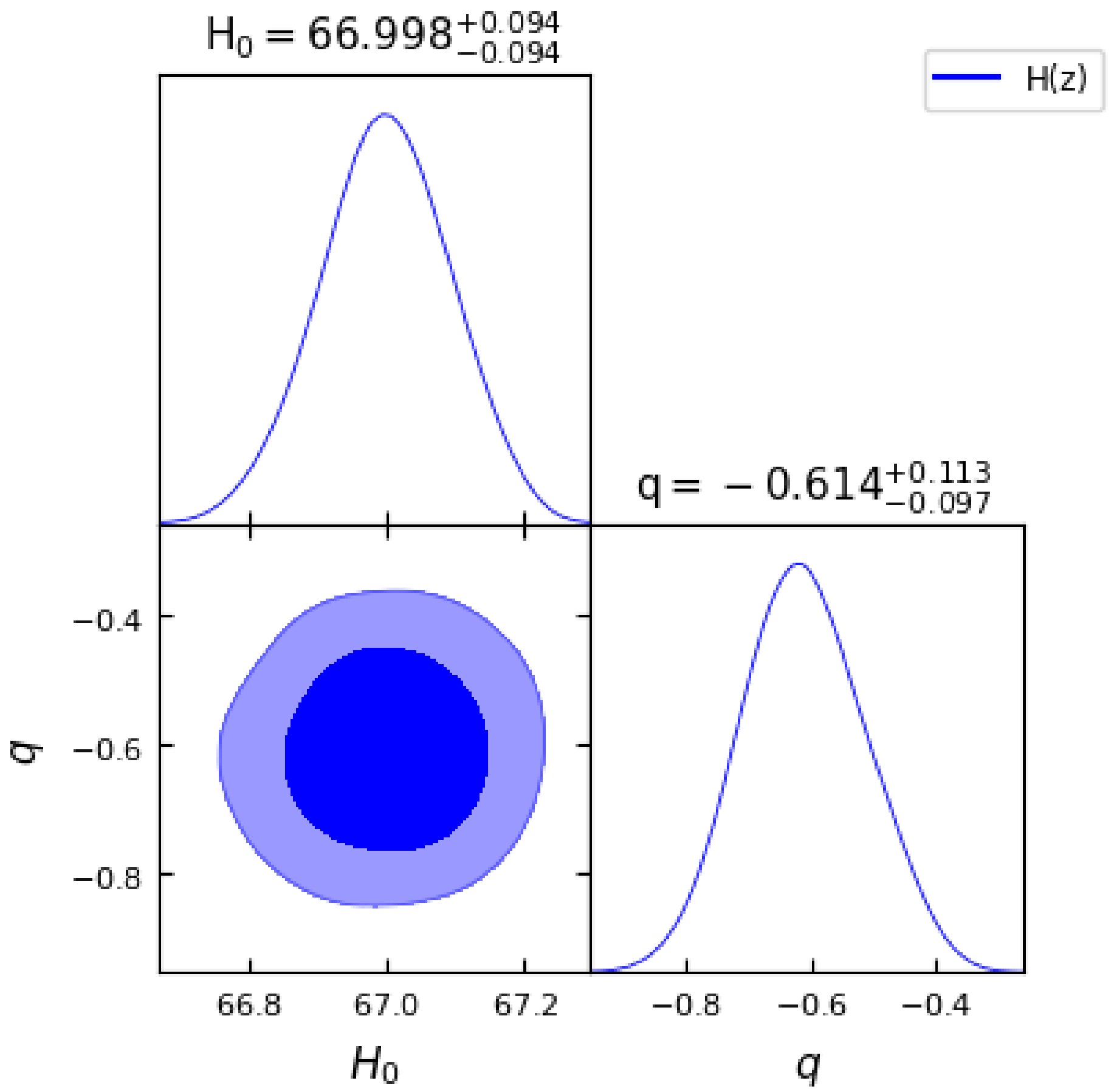
Figure 1. (color online) One-dimensional marginalized distribution and two-dimensional contours using the
$ H(z) $ dataset.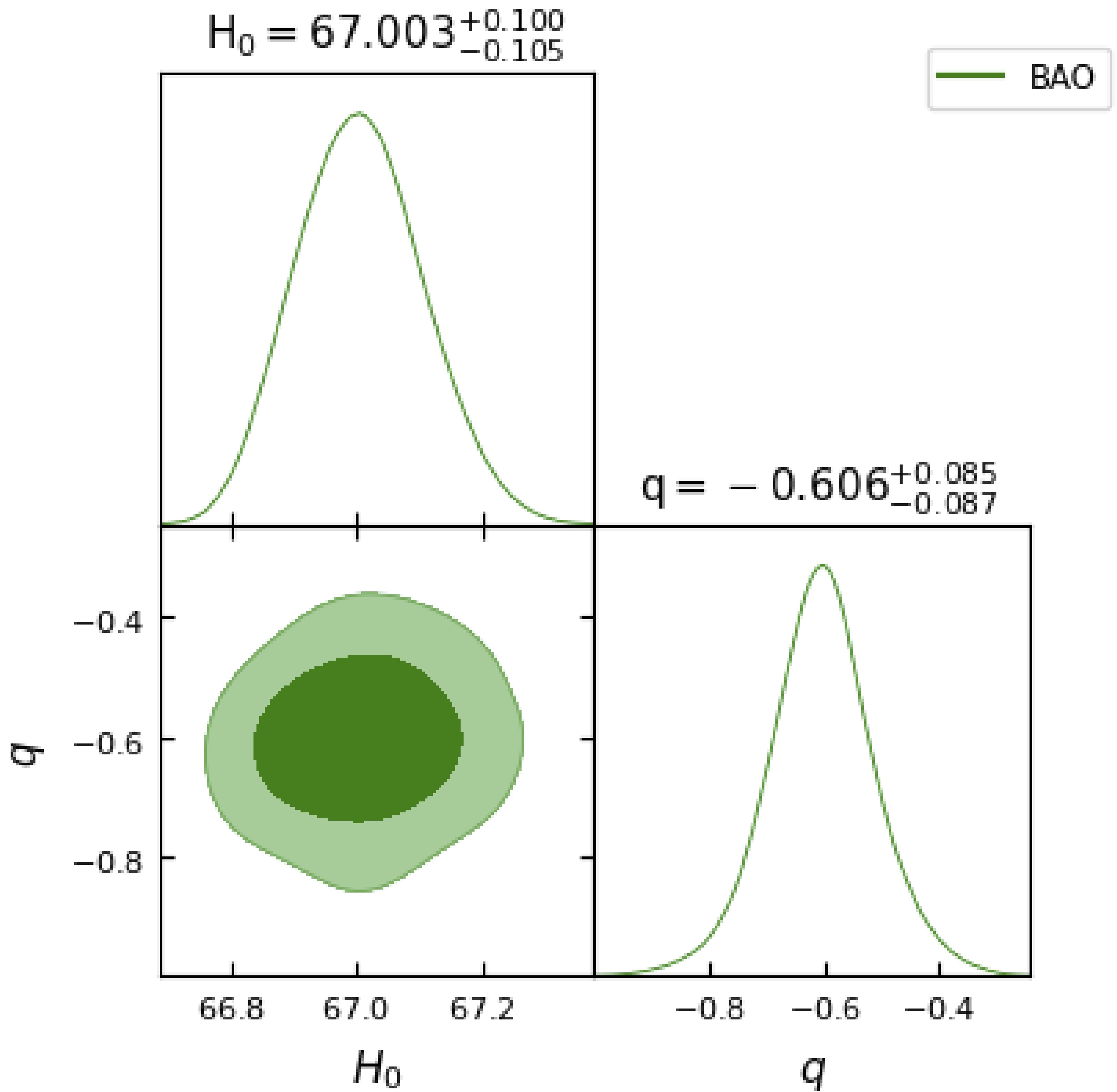
Figure 2. (color online) One-dimensional marginalized distribution and two-dimensional contours using the BAO dataset.
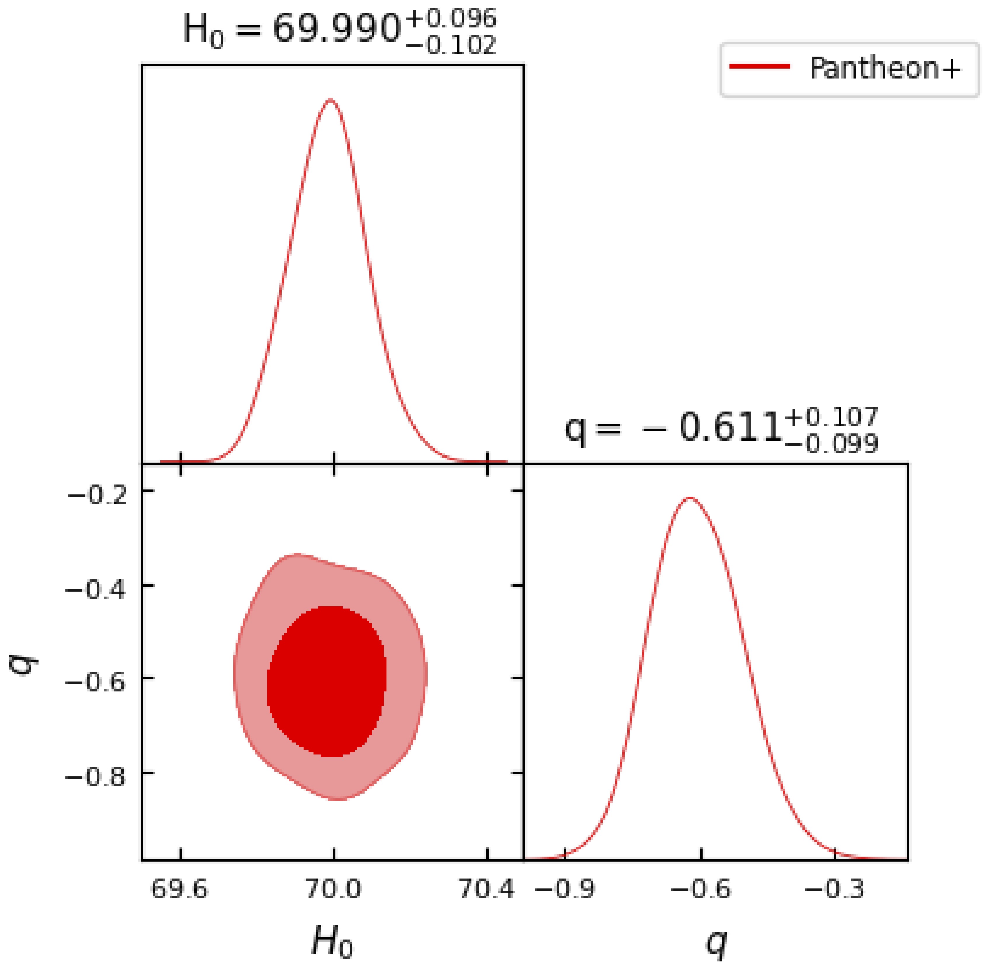
Figure 3. (color online) One-dimensional marginalized distribution and two-dimensional contours using the Pantheon dataset.
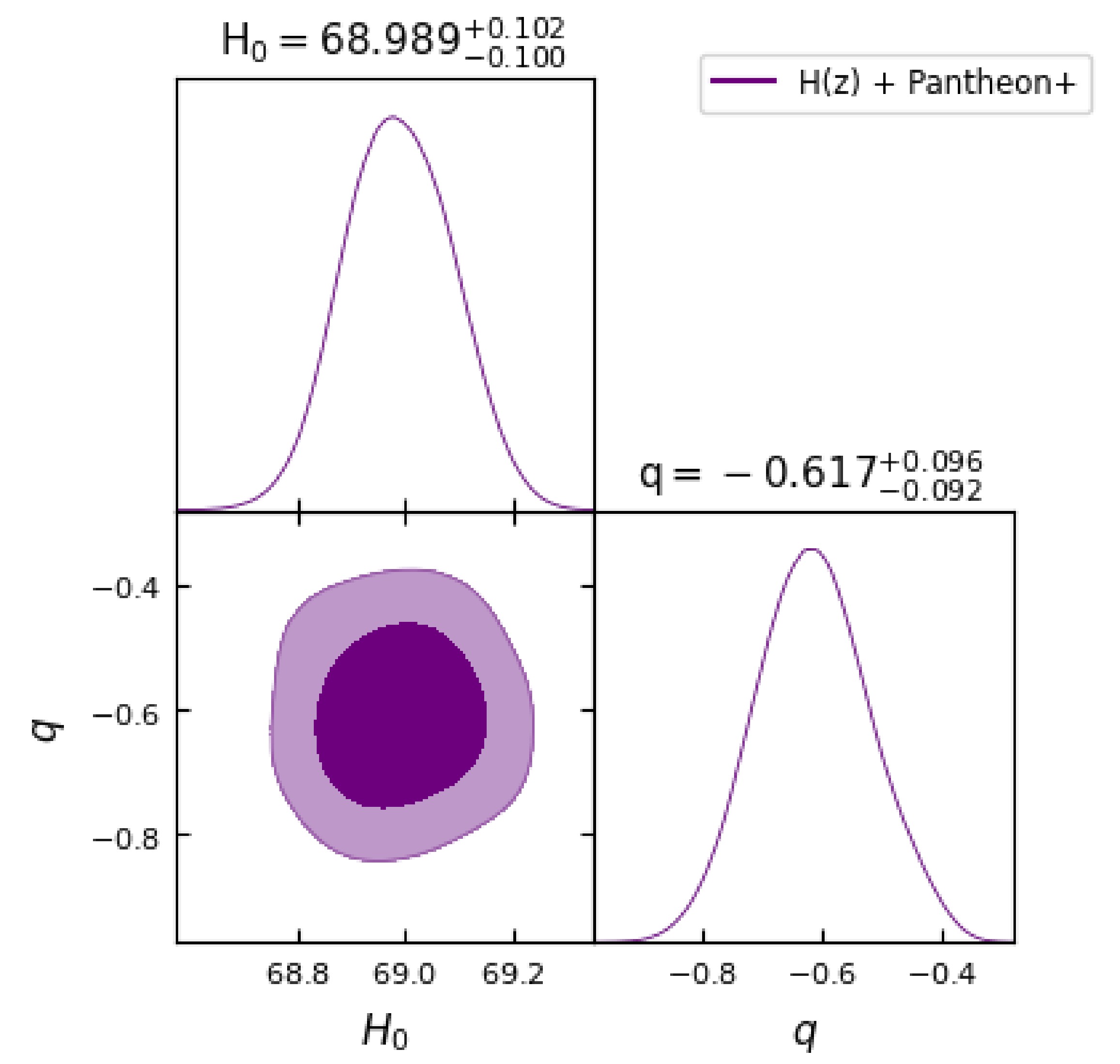
Figure 4. (color online) One-dimensional marginalized distribution and two-dimensional contours using the combination of
$ H(z) $ and Pantheon+ dataset.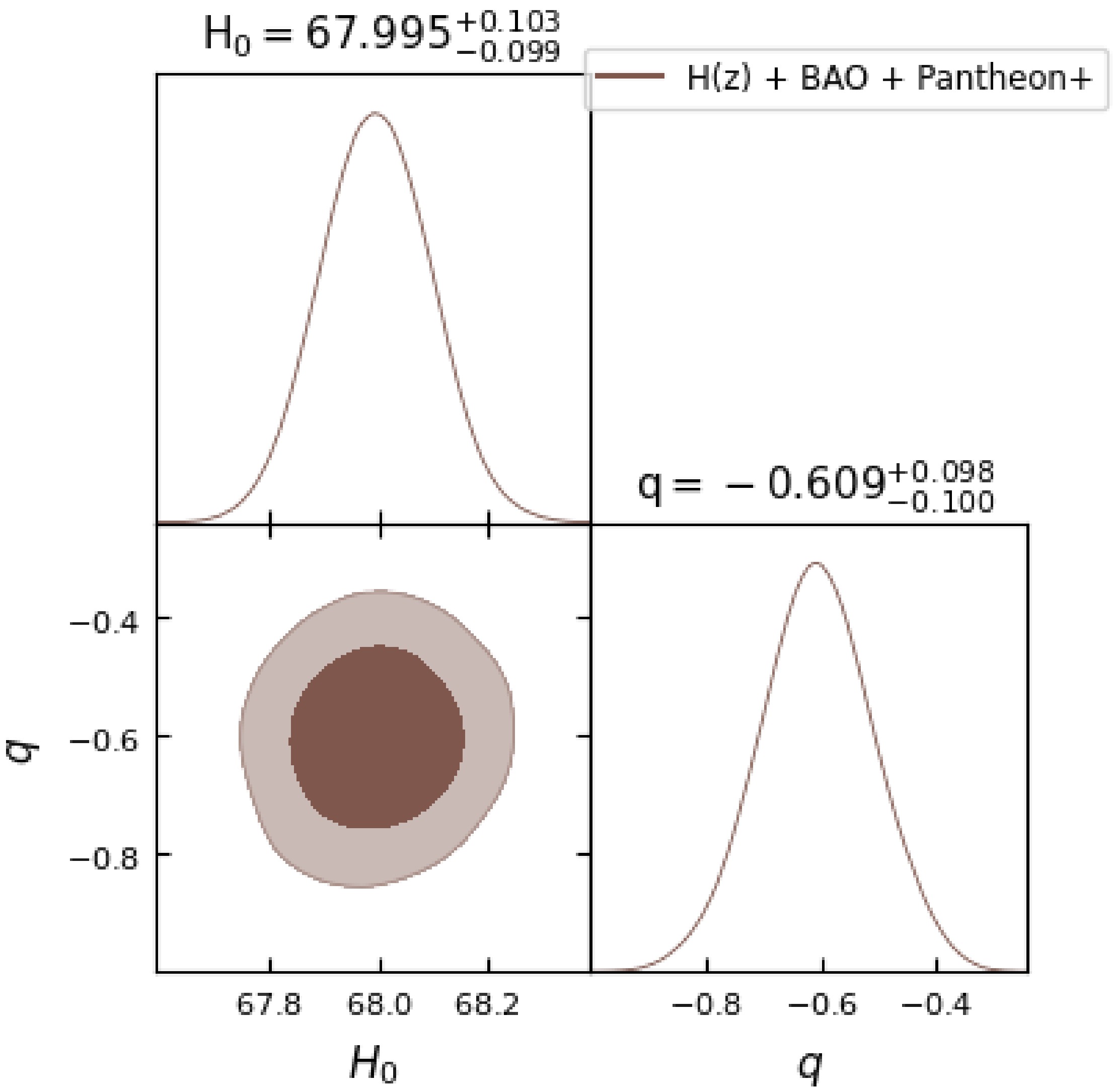
Figure 5. (color online) One-dimensional marginalized distribution and two-dimensional contours using the combination of
$ H(z) $ , BAO, and Pantheon datasets.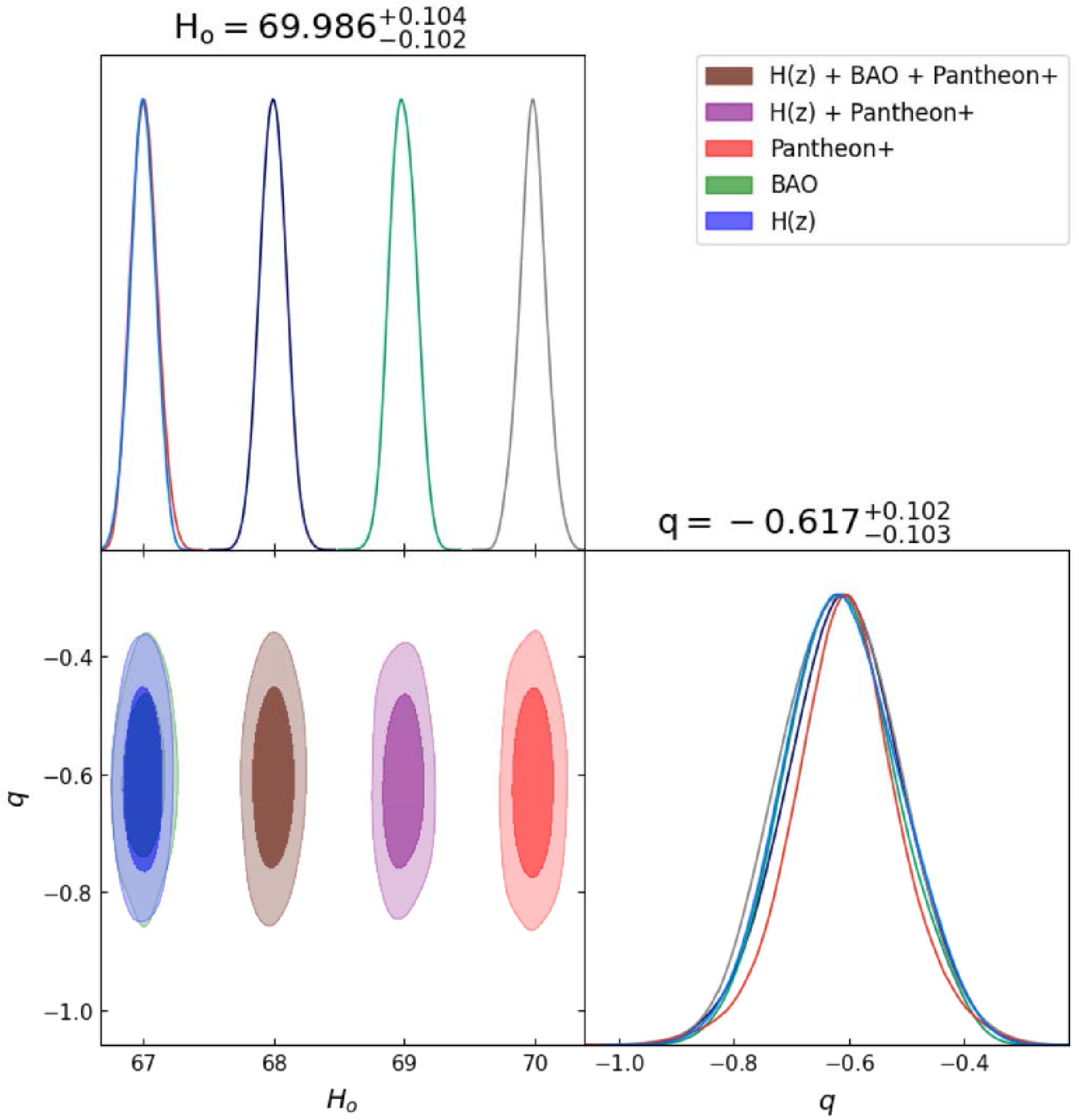
Figure 6. (color online) One-dimensional marginalized distribution and two-dimensional contours using the combined variability across all dataset combinations.
Parameter H(z) BAO Pantheon+ $ H(z)_1 $ 

$ H(z)_2 $ 

$ H_0 $ 

$ 66.998^{+0.094}_{-0.094} $ 

$ 67.003^{+0.100}_{-0.105} $ 

$ 69.990^{+0.096}_{-0.102} $ 

$ 68.989^{+0.102}_{-0.100} $ 

$ 67.995^{+0.103}_{-0.099} $ 

q $ -0.614^{+0.113}_{-0.097} $ 

$ -0.606^{+0.085}_{-0.087} $ 

$ -0.611^{+0.107}_{-0.099} $ 

$ -0.617^{+0.096}_{-0.092} $ 

$ -0.104^{+0.098}_{-0.100} $ 

Table 1. Parameter values exstructed from different datasets (i.e.,
$ H(z) $ , BAO, Pantheon,$ H(z)_1=H(z) $ + Pantheon,$ H(z)_2=H(z) $ + BAO + Pantheon). Here, we have used MCMC and Bayesian analysis.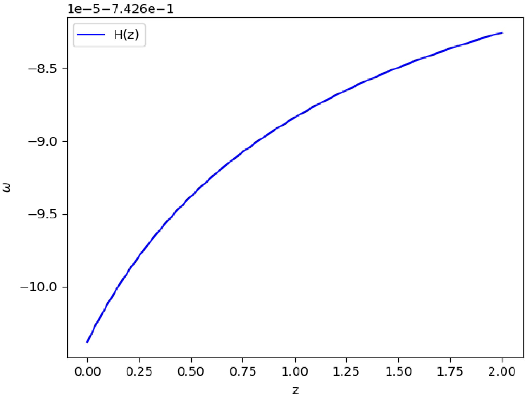
Figure 9. (color online) Variation in the equation of state parameter (ω) vs the redshift (z), which demonstrates that dark energy contributes to the accelerated expansion of the Universe with slight variations with the redshift, thus potentially leading to interesting cosmological consequences.
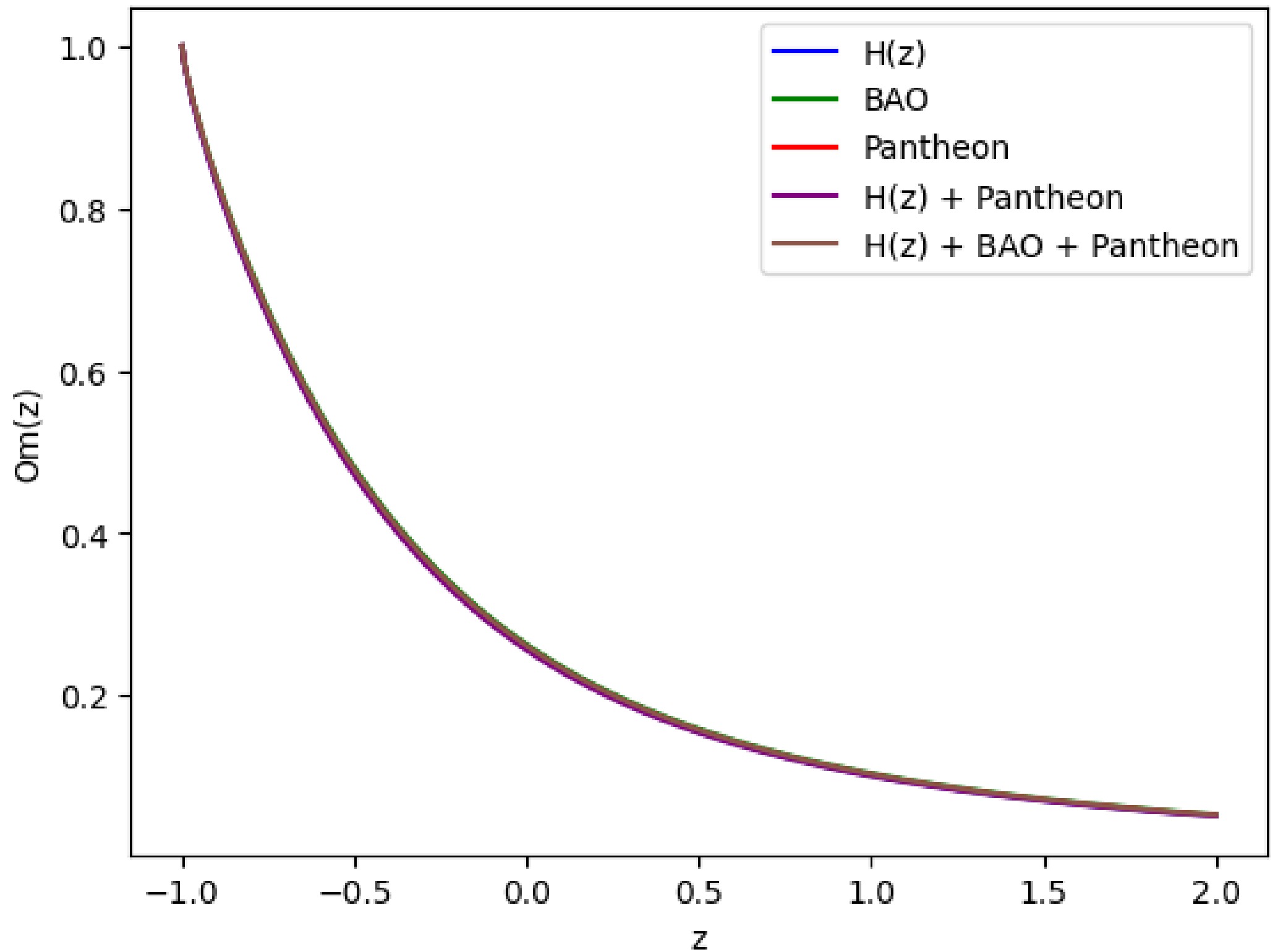
Figure 11. (color online) Variations in
$ Om(z) $ with z across for different combined datasets by considering the β values obtained from each dataset.
Figure 12. (color online) Features of jerk parameter j vs z. Here, the values of j at z = 0 are as follows: for
$ H(z) $ = 7.127$ s^{-3} $ , for BAO = 6.663$ s^{-3} $ , for Pantheon = 6.731$ s^{-3} $ , for$ H(z) $ + Pantheon = 7.387$ s^{-3} $ , and for$ H(z) $ + BAO + Pantheon = 6.997$ s^{-3} $ 
Figure 13. (color online) Features of lerk parameter l vs z.
Figure 14. (color online) Features of snap parameter s vs z.
-
Energy conditions (ECs) or similar cosmic principles explain the distribution of matter and energy across the Universe. They are based on Einstein's gravitational equations and replicate the rules of the cosmos. These circumstances indicate the distribution of matter and energy in space. Hence, the ECs can be expressed as follows:
(i) Weak Energy Condition (WEC):
$ \rho \geq 0 $ ,$\rho+p \geq 0,$ (ii) Null Energy Condition (NEC):
$ \rho + p \geq 0 $ ,(iii) Strong Energy Condition (SEC):
$ \rho + 3p \geq 0 $ ,(iv) Dominant Energy Condition (DEC):
$ \rho - p \geq 0 $ .All the ECs separately and jointly are shown in Figs. 15−19 using the Bayesian analysis of the parameters. Except for the SEC, our results show that the NEC, WEC, and DEC are all satisfied. The SEC violation is justified by the Universe's fastest growth. Therefore, the
$ f(R,G) $ theory of gravity has potential to explain the current scenario of the late-time acceleration without requiring the cosmological constant and dark energy component in the energy budget of the Universe. The distribution of energy density ρ with respect to time t is shown in Fig. 7, whereas the distribution of the pressure is shown in Fig. 8.
Figure 15. (color online) Weak Energy Condition (WEC) vs the redshift (z) for all the combined datasets.
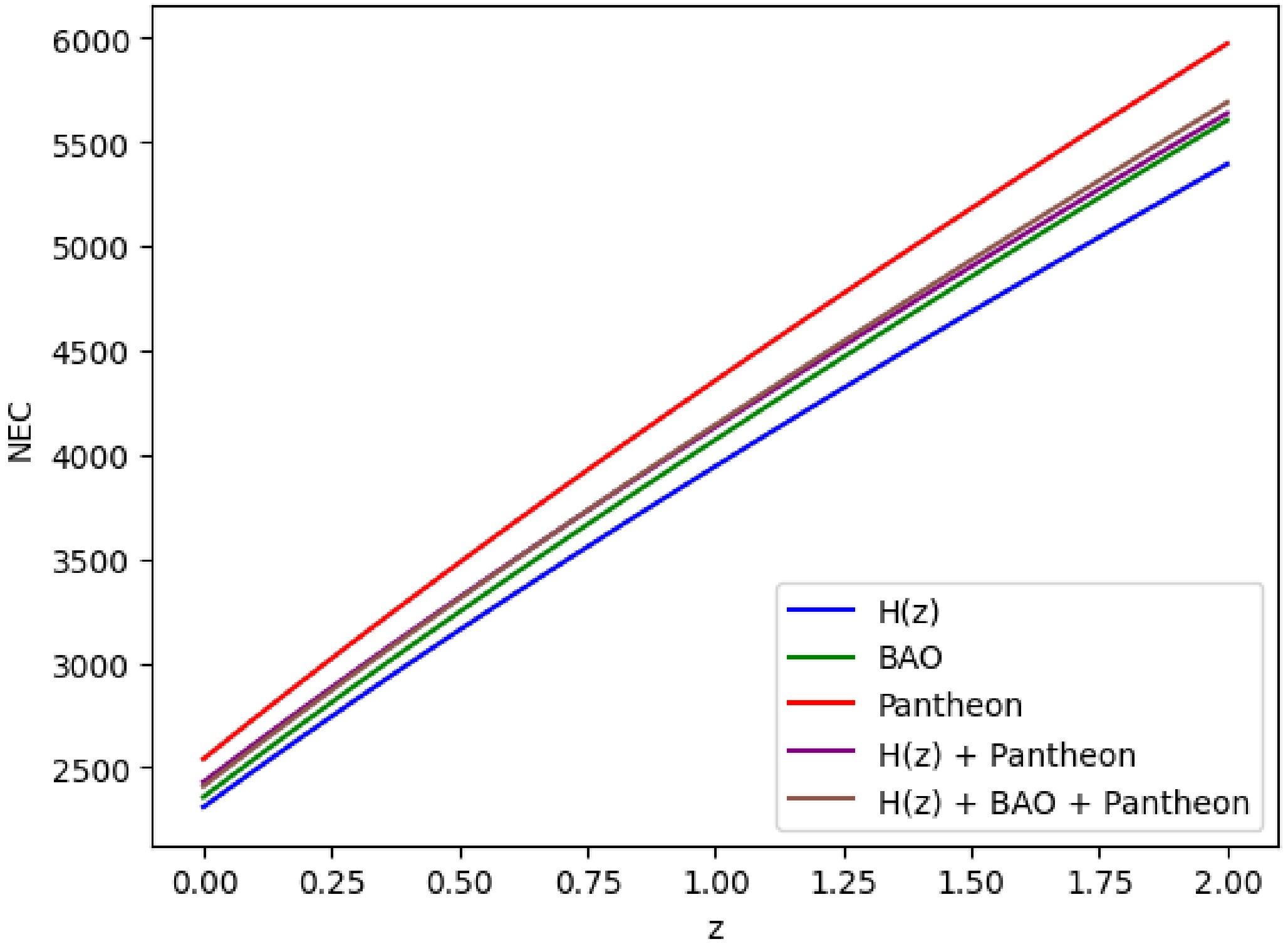
Figure 16. (color online) Null Energy Condition (NEC) vs the redshift (z) for all the combined datasets.
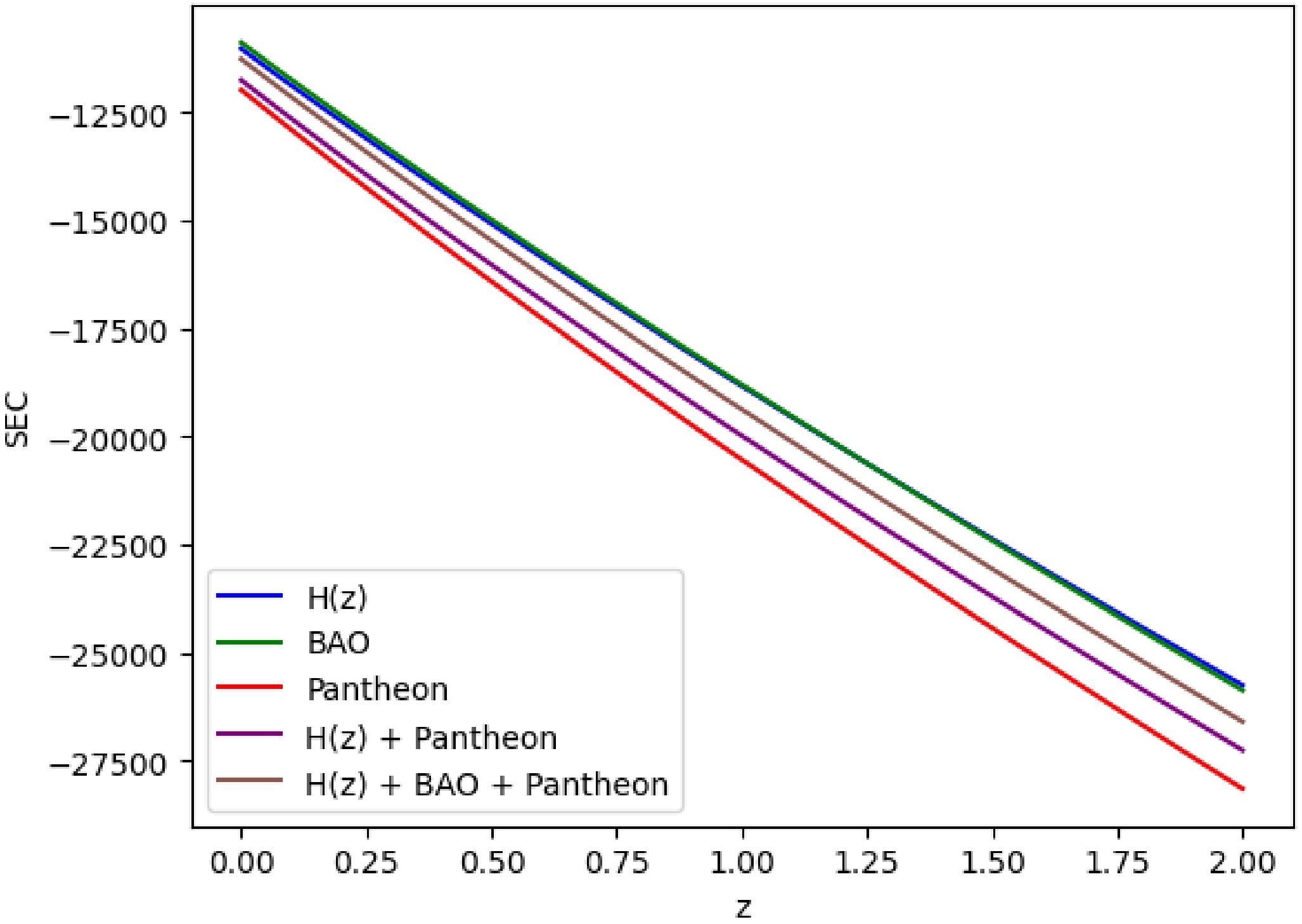
Figure 17. (color online) Strong Energy Condition (SEC) vs the redshift (z) for all the combined datasets.
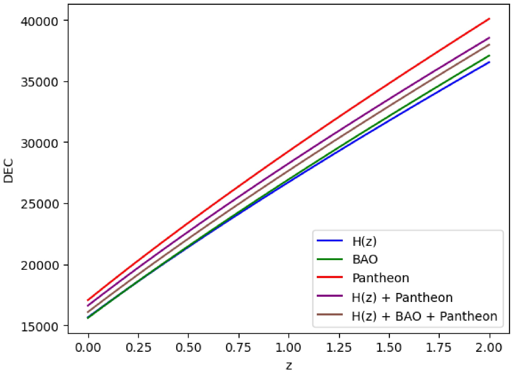
Figure 18. (color online) Dominant Energy Condition (DEC) vs the redshift (z) for all the combined datasets.
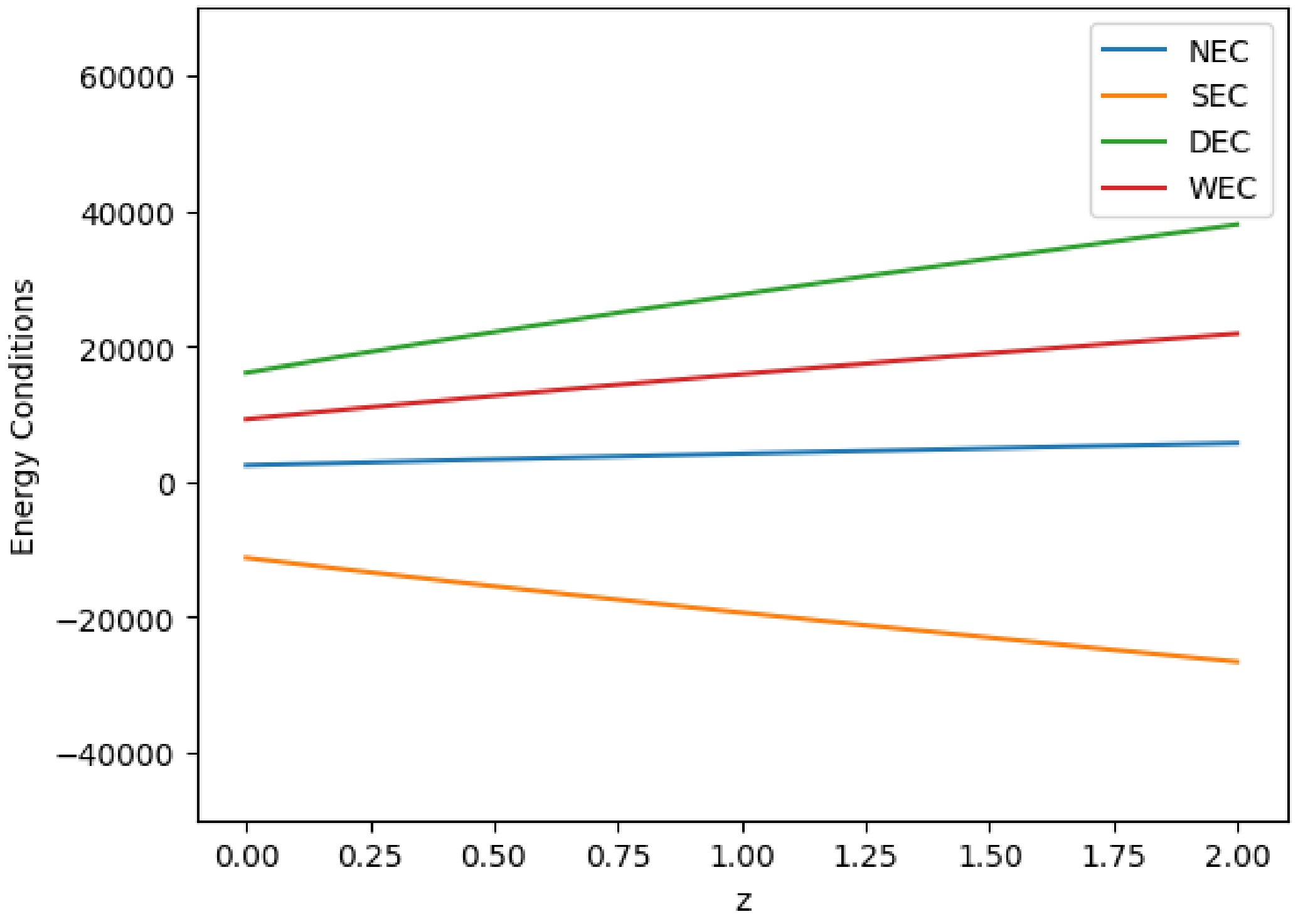
Figure 19. (color online) All energy conditions vs time.
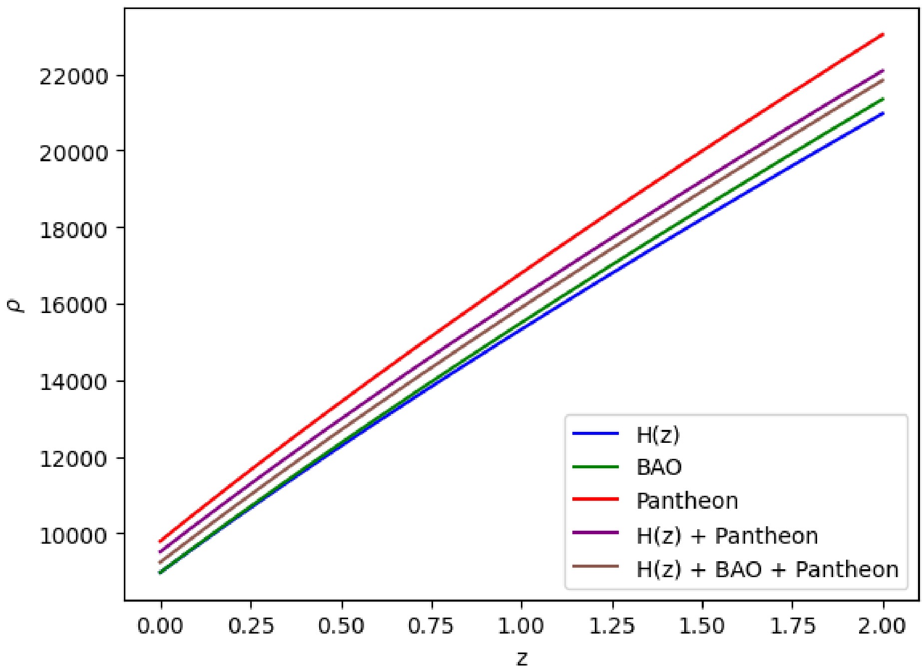
Figure 7. (color online) Dynamic variation in the energy density (ρ) over the redshift (z) under various parameter conditions derived from distinct combinations of the
$ H(z) $ , BAO, and Pantheon datasets.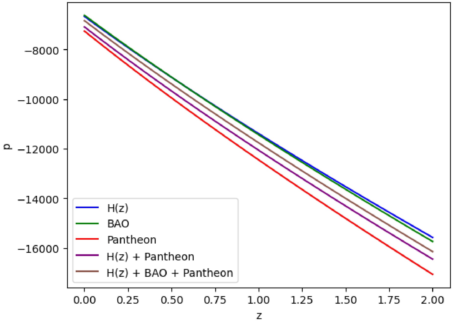
Figure 8. (color online) Dynamic variation of the pressure (p) over the redshift (z) under various parameter conditions derived from distinct combinations of the
$ H(z) $ , BAO, and Pantheon datasets. -
When assessing various dark energy hypotheses in academic works, researchers commonly use state finder parameters
$ r - s $ and the Om diagnosis. The important$ Om(z) $ parameter is formed when Hubble parameter H and cosmic redshift z combine, which can be defined as$ Om(z) = \frac{\Big[\dfrac{H(z)}{H_0}\Big]^2 - 1}{(1+z)^3 - 1}, $

(23) where
$ H_0 $ corresponds to the current value of the Hubble parameter. According to Shahalam et al. [94], the negative, zero, and positive values of$ Om(z) $ indicate the quintessence ($ \omega \ge -1 $ ), ΛCDM, and phantom ($ \omega \le-1 $ ) dark energy hypotheses, respectively.The
$ Om(z) $ parameter can be provided for our model as follows:$ Om(z) = \frac{(1+z)^{2/b}-1}{(1+z)^3-1}. $

(24) -
Many cosmological parameters, given as higher-order derivatives of the scalar component, are examined to comprehend the Universe's expansion history better. Consequently, these characteristics are extremely useful for investigating the dynamics of the cosmos. For example, Hubble parameter H depicts the Universe's expansion rate, q depicts the Universe's phase transition, whereas jerk parameter j, snap parameter s, and lerk parameter l are required to study dark energy theories and their dynamics. These are expressed as follows:
$ \begin{aligned} H = \frac{\dot{a}}{a}, \end{aligned} $

(25) $ \begin{aligned} q = \frac{\ddot{a}}{aH^2}, \end{aligned} $

(26) $ \begin{aligned} j = \frac{\dddot{a}}{aH^3}, \end{aligned} $

(27) $ \begin{aligned} s = \frac{\dddot{a}}{aH^4}, \end{aligned} $

(28) $ \begin{aligned} l = \frac{\ddddot{a}}{aH^5}. \end{aligned} $

(29) -
Basically, state finder diagnostics aid us in obtaining the hidden features of the status of dark energy and thus mysteries attached to the history of the Universe. As we employ a cosmic compass, these diagnostics lead us through the complexities of cosmic evolution. Parameters r and s are used in state finder diagnostics. Using these characteristics, we can gain a better understanding of the evolution of the Universe. We consider them as cosmic metres that offer data on the expansion of the Universe and its constituent components. These are basically dimensionless parameters that encapsulate the essence of the cosmic development and thus serve as a filter to aid in our understanding of the underlying dynamics of the Universe.
Now, the general mathematical expression for the required parameter, expressed in terms of H, is expressed as follows:
$ \begin{aligned} r = \frac{\ddot{\dot{a}}}{aH^3}, \end{aligned} $

(30) whereas the equations for r and s in our model, when expressed in terms of q, become
$ \begin{aligned} r = 2q^2 + q, \end{aligned} $

(31) $ \begin{aligned} s = \frac{-1 + r}{3(-\dfrac{1}{2}+q)}. \end{aligned} $

(32) The scale factor trajectories in the resulting model is shown in Fig. 10 to follow a specific set of paths. Our strategy is consistent with the results for the cosmic diagnostic pair from power law cosmology. The pioneer investigations on state finders are described in Refs. [95−106]. The evolutionary trajectory in the
$ r - s $ plane of state finders pairs aids us in enhancing the accuracy of the model and its classification among various type of dark energy models, as discussed in Refs. [95−106]. The behaviors of the proposed model$ r - q $ ,$ s - q $ , and$ r - s $ planes are depicted in Fig. 10. From Fig. 10, we observe that the proposed model behaves like the SCDM model$ (r = 1, s = 1) $ at the initial epoch and approaches toward the ΛCDM model$ (r = 1, s = 0) $ at late time.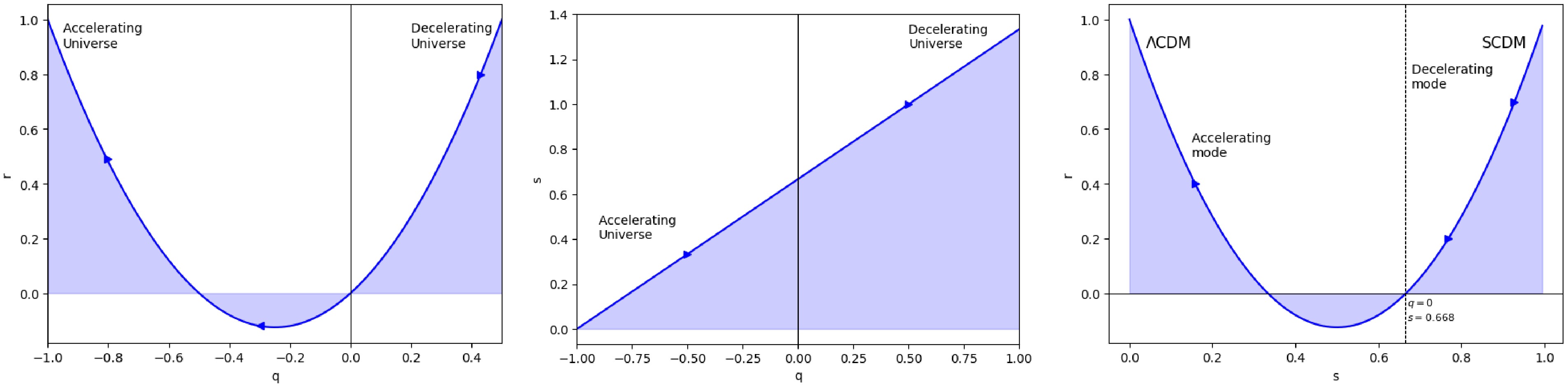
Figure 10. (color online) Features of the state finder plots of
$ r-q $ ,$ s-q $ , and$ r-q $ . -
The motivation of this study was to examine Ricci scalar R and Gauss-Bonnet invariant G to characterize a cosmological model in flat space-time via
$ f(R,G) $ gravity. We aimed to investigate the observational limitations under a power law cosmology that relies on two parameters, the Hubble constant ($ H_0 $ ) and deceleration parameter (q) utilizing the 57-point$ H(z) $ data, 8-point BAO data, 1048-point Pantheon data, joint data of$ H(z) $ + Pantheon, and joint data of$ H(z) $ + BAO + Pantheon. The outcomes for$ H_0 $ and q are realistic within observational ranges. Our estimate of$ H_0 $ is remarkably consistent with various recent Planck Collaboration studies under the ΛCDM model.Through several graphical demonstrations (Figs. 1−19 and Table 1) , we showed that the obtained values for
$ H_0 $ by bounding the proposed model with OHD, BAO, and Pantheon compilation of SNIa data satisfactorily favor its corresponding value observed in the Plank collaboration [84]. In addition to these graphical presentations, we analyzed the model by studying the energy conditions, jerk parameter, lerk parameter, Om diagnostics, and state finder diagnostic tools. According to our study, the power law cosmology within the context of$ f(R,G) $ gravity provides the most comprehensive explanation for the important aspects of cosmic evolution. Furthermore, at the final stage of this paper, we analyzed the research of Singh et al. [79] that prescribes a cosmological model with the power law under the framework of the modified theory with a higher order curvature term. They [79] obtained$ H_{0} = 68.119^{+0.028}_{-0.12} $ $\rm km\; s^{-1}Mpc^{-1}$ ,$ q = -0.109^{+0.014}_{-0.014} $ ;$H_{0} = 70.5^{+1.3}_{-0.98}$ $\rm km\; s^{-1} Mpc^{-1}$ ,$ q = -0.25^{+0.15}_{-0.15} $ and$ H_{0} = 69.103^{+0.019}_{-0.10} $ $\rm km\; s^{-1} Mpc^{-1}$ ,$ q = -0.132^{+0.014}_{-0.014} $ using$ H(z) $ data, Pantheon+ compilation of SNIa data, and joint data of$H(z) $ + Pantheon+, respectively. In this paper, the constrained values from the proposed model are as follows:$ H_0 = 68.001^{+0.093}_{-0.087} $ km s$ ^{-1} $ Mpc$ ^{-1} $ ,$ q = -0.106^{+0.009}_{-0.009} $ ;$ H_0 = 67.973^{+0.101}_{-0.105} $ km s$ ^{-1} $ Mpc$ ^{-1} $ ,$ q = -0.099^{+0.010}_{-0.010} $ ;$ H_0 = 67.995^{+0.086}_{-0.111} $ km s$ ^{-1} $ Mpc$ ^{-1} $ ,$ q = -0.100^{+0.010}_{-0.010} $ ;$ H_0 = 67.980^{+0.012}_{-0.097} $ km s$ ^{-1} $ Mpc$ ^{-1} $ ,$q = -0.110^{+0.010}_{-0.011}$ ;$ H_0 = 68.018^{+0.093}_{-0.104} $ km s$ ^{-1} $ Mpc$ ^{-1} $ ,$q = -0.104^{+0.010}_{-0.011}$ using$ H(z) $ data, 8-point BAO data, 1048-point Pantheon data, joint data of$ H(z) $ + Pantheon and joint data of$ H(z) $ + BAO + Pantheon, respectively. As a suitable methodology, the welknown and effectiveMCMC was uniquely employed in this study.Note that the proposed model minimized
$ H_{0} $ tensions and it is calibrated using only$ 0.68 \sigma $ ,$ 1.19 \sigma $ ,$ 1.191 \sigma $ ,$ 1.23 \sigma $ , and$ 1.17 \sigma $ for$ H(z) $ data, 8-point BAO data, 1048-point Pantheon data, joint data of$ H(z) $ + Pantheon, and joint data of$ H(z) $ + BAO + Pantheon, respectively, when we analyzed the estimated values of$ H_{0} $ in this paper with the value of$ H_{0} $ obtained by the Plank Collaboration [4]. Moreover, because of the constant value of q in power-law cosmology, it cannot describe the red-shift transition, and the proposed model fails to explain the early deceleration phase of the Universe. However, we can describe the early deceleration phase of the Universe by selecting an appropriate value of ζ in$q = {1}/{\zeta} - 1$ . However, note that the model fails to explain the late-time acceleration of the Universe.Finally, although we obtained many useful features, the power-law cosmology appears to be not a completely packagable technique to study to entire dynamics and eventual fate of the Universe. However, this connection may have some scope to explore thermodynamical aspects, particularly entropy, of the late-time acceleration of the Universe, and the works in Refs. [79, 107, 108] may be addressed in future projects.
Modified power law cosmology: theoretical scenarios and observational constraints
- Received Date: 2024-05-07
- Available Online: 2025-04-15
Abstract: This research paper examines a cosmological model in flat space-time via


 DownLoad: