High-precision inverse potentials for neutron-proton scattering using piece-wise smooth Morse functions

Current high-precision nucleon-nucleon potentials, available for scattering data up to about the pion-threshold of 350 MeV, are given by various groups, such as Argonne $ v_{18} $ [1], Bonn potentials [2], Reid [3], Nijmegen [4] and Paris [5]. All of these have modeled the NN interaction to consist of One Pion Exchange Potential for long inter-nuclear distances of r ≥ 2 fm. The main differences between these high precision potentials stem from the way nucleon-nucleon interaction is modeled, for the intermediate/medium (1.0 fm < r < 2 fm) and the short-range (r < 1.0 fm) [6]. These are modeled using a central potential along with an interplay of orbital, tensor, spin-orbit, and quadratic spin-orbit terms. The approach involves simultaneously solving for the wave-functions based on the model potential and optimizing, close to between 40-50, parameters for obtaining the phase shifts for all the ℓ-channels for the nucleon-nucleon scattering from which the total cross sections are predicted to match the experimental ones [7]. An alternative methodology is to construct the inverse potentials utilizing the phase function method or Variable Phase Approximation [8–10], which has the advantage of obtaining phase shifts directly utilizing the potential without recourse to the wave-function. Here, the second-order time-independent Schrödinger equation is transformed into a set of independent first-order non-linear Ricatti equations for each ℓ channel. So, one can determine the potentials corresponding to phase shifts for individual channels. This methodology is equivalent to constructing the model potential directly from the available scattering phase shifts data, which is the basic premise of the machine learning paradigm [11].

Typically, to obtain a complete inverse scattering solution, both N discrete bound state energies $ E_n < $ 0 (n = 1, 2, $ \ldots $, N) and all possible scattering phase shifts for energies E > 0, all the way up to $ \infty $, are ideally required [12]. But, typically the experimental data available is limited to very few projectile energy values. Hence neural network-based machine learning models are not suitable and we propose to utilize meta-heuristic genetic algorithms for constructing model potentials by optimizing the parameters of the chosen reference function to guide the process. The phase equation arising from the phase function method is incorporated in the optimization procedure and the bounds for various parameters are chosen to obtain physically relevant potentials. This is exactly the spirit of physics-informed machine learning [14] which is the way forward for solving complex problems in computational sciences.

Selg [12, 15] proposed the Morse function as an ideal choice for the reference function to construct inverse potentials due to its various advantages. It has the analytical solution of time-independent Schrödinger equation for ℓ=0 and the nature of Morse function has all the characteristics of nucleon-nucleon interaction such as repulsion at short inter-nuclear distances, attraction at intermediate, and quickly falling tail for large distances. Previously, inverse potentials for all ℓ channels of np scattering have been constructed using phase function method by taking the Morse function as a zeroth reference [16]. The Deuteron structure and form factors have been determined from the analytical ground state wavefunction [17]. These were achieved by implementing an innovative algorithm based on a variation of the Variational Monte-Calro technique [18], which was cast as an optimization routine. It was an equivalent alternative to the least squares minimization approach.

One can observe the complex nature of nucleon-nucleon interaction, as envisaged by various groups who have obtained realistic precision potentials, which consist of very different characteristics for the three regions. So, we have realized that considering a single Morse function limits the space of curves available for convergence to the required inverse potentials.

In principle, one can construct inverse potentials by solving phase equation, for a potential $ V(r) $, iteratively within the machine learning-based optimization algorithm. The idea is to start with an initial potential array $ V[i] = V[r_{i}] $. Here, $ r_i $ is an array of uniformly sampled values in an interval between $ [0, r_f] $, where $ r_{f} $ is the distance beyond which the interaction is assumed to be negligible. One can initialize the potential value $ V_{i} $ at various points $ r_{i} $ randomly, just as one would initialize the wavefunction values $ \psi_{i} $ at various $ r_{i} $ in Variational Monte Carlo approach for determining the ground state energy of a physical system [19]. But, here is an important difference between solving the time-independent Schrödinger equation and phase equation. While the wavefunction and its second derivative are evaluated in every iteration to determine energy in the Variational Monte Carlo approach using the Hamiltonian of time-independent Schrödinger equation, the potential appears in the phase equation only as a multiplicative function. So, while solving the time-independent Schrödinger equation ensures the evolving wavefunction solution to remain smooth, the resulting potential from the phase equation does not. Thus, we need to rely upon certain smooth mathematical functions as a reference for initializing the algorithm. The variation of parameters of the reference function would generate a large number of curves in the sample space. The nature of the curves will depend on the bounds chosen for each of the individual parameters of the reference potential. The inverse potential that best describes the expected phase shifts is obtained by optimizing the parameters of the reference function by minimizing a cost function such as mean squared error. The methodology of constructing inverse potentials by solving the phase equation utilizing the reference function is called the reference potential approach [12]. Generally, a good choice for this purpose is a multi-component potential composed of smoothly joined Morse type, i.e. piece-wise smooth Morse function [12]. A three-component Morse potential was successfully utilized by Selg [20] for obtaining the molecular interaction potentials.

In this paper, we have considered the same reference to construct the inverse potentials for various ℓ-channels of np scattering for energies up to 350 MeV. Using such a choice, we have not only numerically solved the phase equation for single-channel scattering for various ℓ-channels but also successfully implemented the "Stapp-Parametrization" to incorporate mixing parameters, for many-channel scattering [10]. This latter involves solving three coupled non-linear differential phase equations. Our computational approach involves solving these single and coupled differential equations iteratively within a genetic algorithm based optimization routine [21] to obtain the best parameters for the piece-wise smooth Morse curve, consisting of three functions, to minimize mean squared error as the cost function.

In this section, we explain the necessary models used in the paper. We demonstrate the non-linear relationship between observables and the scattering potential, focusing on nuclear scattering experiments. Following this, we elaborate on the Reference Potential Approach (RPA), where we employ a piece-wise Morse function as a reference to solve the non-linear equations. Subsequently, we discuss the machine learning-based optimization algorithm used to optimize model parameters, resulting in high-precision neutron-proton interaction potentials.

To represent the forward problem of nuclear scattering, one must solve the $ 3D $ time-independent Schrödinger equation [22]. This is a linear, second-order partial differential equation that describes the evolution of the $ \psi(r) $ wave functions under a scattering potential $ V(r) $. The problem can be simplified into solving the radial Schrödinger equation, which is defined as:

Where $ k=\sqrt{\dfrac{2\mu E_{cm}}{\hbar^2}} $, $ U(r) =\dfrac{2\mu V(r)}{\hbar^2} $ and μ is reduced mass of the system.

The $ E_{cm} $ is related to $ E_{\ell ab} $ by the relation $ E_{cm} = \dfrac{m_{T}}{m_{T}+m_{P}}E_{\ell ab}. $ Here, $ m_{T} $ and $ m_{P} $ are masses of target and projectile respectively. In scattering experiments, we concentrate on the asymptotic nature of wave functions, which are the sum of an incoming plane wave $ e^{ikr} $ and an outgoing spherical wave, weighted by the scattering amplitude $ f(k,\theta) $ and related to the differential cross section as [22]

The scattering amplitude and phase shifts can be expressed using a partial wave expansion, resulting in the following form [22]:

where $ P_{\ell} $ is the $ \ell^{th} $ order Legendre polynomial and $ \delta_{l\ell} $ is the phase shift of the $ \ell^{th} $.In scattering experiments, differential and total cross sections are measured, and phase shifts are obtained by fitting different partial waves. So therefore, solving Schrödinger equation by fitting the expected asymptotic wavefunction, and obtain the phase shifts is the forward problem.

However, the Variable Phase Approximation or Phase function method addresses the inverse problem, where the linear homogeneous equation of the second order can be reduced to the first order- the Ricatti equation. This approach suggests that a function fulfilling the Riccati equation, known as a phase function, represents the phase shift of the wave function at each point during scattering by a potential that is truncated at that point, compared to the case of unhindered motion [10, 23]. Now, we will discuss an exact equation for phase functions, which is helpful when performing actual numerical computations. The most important cases associated with potential scattering are considered.

Consider elastic scattering by a central potential or an arbitrary potential that does not result in mixing of partial waves with different orbital angular moments (i.e., one-channel reaction). For this, the second order TISE is transformed into Ricatti type equation [9, 10, 24] which is given by

where $ U(r)=\dfrac{2\mu V(r)}{\hbar^2} $.

The initial point for the phase equation is $ \delta_{\ell}(r = 0) = 0 $, indicating zero phase shift, where the potential hasn't yet affected the incoming wave. The ultimate phase shift measured, $ \delta_{\ell}(r \rightarrow \infty) $, represents the accumulated phase shift as the distance approaches infinity. This equation finds utility in atomic and nuclear physics for determining the scattering phase shift corresponding to a specific potential.

The Riccati Hankel function of first kind is related to $ \hat{j_{\ell}}(kr) $ and $ \hat{\eta_{\ell}}(kr) $ by $ \hat{h}_{\ell}(r)=-\hat{\eta}_{\ell}(r)+i\; \hat{j}_{\ell}(r) $. For $ \ell = 0 $, the Ricatti-Bessel and Riccati-Neumann functions $ \hat{j_0} $ and $ \hat{\eta_0} $ get simplified as $ \sin(kr) $ and $ -\cos(kr) $. So phase equation, for ℓ=0 is [18]:

For higher partial waves the Ricatti-Bessel and Riccati-Neumann functions used in PFM can be easily obtained by using following recurrence formulas [16]:

Phase function equation for ℓ=1 & 2 takes following form:

Similarly phase function equations can be obtained for higher partial waves using equations 6 & 7.

Eq. 4 is non-linear equation and can be solved numerically using Runge-Kutta 5th order (RK-5) method with initial condition $ \delta_{\ell}(k,0)=0 $.

The Phase Function Method can be expanded to encompass scenarios involving a non-central tensor interaction and multi-channel inelastic scattering. A notable instance is the elastic scattering interaction between two particles with spin $ 1/2 $, such as nucleons, wherein the tensor interaction is considered. In the triplet spin state, the tensor forces $ T_j(r) $ intermix the partial waves, leading to different orbital angular momenta $ \ell = J \mp 1 $ for a given total angular momentum J of the system. As a result, the equations governing the radial wave functions $ u_J(r) $ and $ w_J(r) $ are interrelated as [10, 22]:

The coupling of equations 10 complicates the calculation of scattering phase shifts, which involves two phase shifts and a mixing component. For small r, one of the system's linearly independent solutions is significantly larger than the other. It is challenging to "extract" the gradually growing solution from the background of the initial solution. The PFM allows us to obtain a straightforward set of first-order linear equations for three functions and eliminating this drawback. It's widely recognized that a tensor potential permits a distinct parametrization of the scattering matrix. Various representations of these parameters within the PFM equations have been developed in studies by Kynch [25], Babikov [26], and Cox and Perlmutter [27].

In this paper, we will focus solely on the equations for the functions $ \delta_{J,J-1}(r) $, $ \delta_{J,J+1}(r) $ and $ \epsilon_{J}(r) $ which are associated with the "Stapp parametrization", widely employed in nuclear physics [26, 28]. In neutron-proton scattering, multiple-channel scattering occurs. For the state with angular momentum J=1, there is a mixing of the $ ^3S_1 $ and $ ^3D_1 $ states with a mixing parameter $ \epsilon_1 $. For J=2, there is mixing of the $ ^3P_2 $ and $ ^3F_2 $ states with a mixing parameter $ \epsilon_2 $. For J=3, there is mixing of the $ ^3D_3 $ and $ ^3G_3 $ states with a mixing parameter $ \epsilon_3 $, and for J=4, there is mixing of the $ ^3F_4 $ and $ ^3H_4 $ states with a mixing parameter $ \epsilon_4 $.

Therefore, the equations for Stapp parameterization can be written for a particular J as:

where $ P_{J,\ell} (r) $ and $ Q_{J,\ell} (r) $ can be defined as

Eq. 11- 13 are three non-linear coupled first order equation which we can be solved using RK -5th order with initial condition $ \delta_{J,J-1}(0) = 0, \; \; \; \delta_{J,J+1}(0) = 0 $ and $ e_{J}(0) = 0 $.

So, in this work, we have studied the single channel and multi- channel scattering using Phase Function method by employing Reference Potential Approach.

Selg[12, 15] suggests reference potential approach for solving 1D quantum systems wherein a single Morse function [12] or a combination of smoothly joined Morse functions of the form

can be chosen as starting point to solve time-independent Schrödinger equation for its energy eigenvalues, scattering phase shifts, and also Jost function, from which one can obtain the inverse potential [12].

Here $ D_i $'s are potential depths at equilibrium distances $ r_i $'s, and $ \alpha_i $'s reflect shape parameter of Morse functions. $ V_i $'s are constants added to total potential, whose importance shall be made clear later. These functions are smoothly joined at various boundary points $ x_{i+1} $.

The number of distinct Morse-type components that may be added is almost unlimited. Naturally, the more components one includes, the better the match with the experimental data, but also more challenging it become to obtain the analytical solution to the problem.

In this paper, we have considered three Morse component (i = 0, 1, 2) to study neutron-proton (n-p) scattering so that they can incorporate all the interaction between the nucleons, given as

where $ x_1 $ and $ x_2 $ are two internal points that demarcate the three potentials, called as boundary points. These are also varied so that a large number of smooth curves would be available from the sample space to look for the best optimal solution. For ensuring smoothness of potential at the boundary points $ x_1 $ and $ x_2 $, in-between the three, the functions $ U_0(r)|_{r=x_1} = U_1(r)|_{r=x_1} $ and $ U_1(r)|_{r=x_2} = U_1(r)|_{r=x_2} $ and their derivatives must be continuous at $ x_1 $ and $ x_2 $. That is,

Using these equations, four of the twelve parameters were determined as

where the factors $ f_0, f_1, g_0, g_1, k_1, k_2, l_1, l_2 $ are given by:

So, we have to optimize eight model parameters of three smoothly joined Morse function i.e. $ \alpha_0 $, $ \alpha_1 $, $ \alpha_2 $, $ r_0 $, $ r_1 $, $ r_2 $, $ V_2 $, $ D_0 $. We have also optimised the points $ x_1 $ and $ x_2 $ where the considering Morse functions are joined. So, overall, we need to optimize 10 parameters to construct inverse scattering potentials for a single channel scattering.

But for many channel scattering, there are three potentials that we need to construct by solving three coupled non-linear first-order equations simultaneously. For this, we need to optimize 30 parameters to get potentials corresponding to different total angular momentum J along with tensor potential.

Hence, we optimized these required parameters by utilizing a physics-informed machine learning paradigm through the variable phase approximation, which is the inverse scattering method.

Manual optimization of parameters is a time-consuming and resource-intensive task, requiring experimentation with various combinations and settings. To expedite this process, optimization algorithms [29] are employed to efficiently determine the best configuration of model parameters. These algorithms iterate through numerous combinations to identify the optimal model configuration, surpassing the capabilities of human optimization.

In machine learning optimization, a loss function serves as a metric for assessing the disparity between actual and predicted output values. The objective is to reduce the error captured by the loss function, thereby enhancing the model's accuracy in predicting outcomes.There are various techniques that we may utilize to optimize a model. In this study, we employed a prominent optimization technique known as the Genetic Algorithm (GA) [21, 30, 33]. GA is an optimization method inspired by Genetics and Natural Selection. It's commonly employed to discover optimal or close-to-optimal solutions for challenging problems that might otherwise be impractical to solve within a reasonable time-frame. It is commonly used in research for solving optimization problems. While GAs do not necessarily involve explicit learning processes like those found in supervised or reinforcement learning, they utilize principles inspired by biological evolution to iteratively improve candidate solutions to optimization problems. In Genetic Algorithms, a pool or population of potential solutions is subjected to recombination and mutation, similar to processes observed in natural genetics. This generates new offspring, and the cycle repeats across multiple generations. Each individual, representing a candidate solution, is evaluated based on its fitness, determined by the objective function value. Fitter individuals have a higher likelihood of reproducing, following the principle of 'Survival of the Fittest' from Darwinian Theory [21, 29].

Through successive generations, the algorithm evolves better solutions until a stopping criterion is met. While GAs involve randomness, they outperform simple random local search methods by leveraging historical information.

Process of GA The genetic algorithm employs three primary sets of rules during each iteration to generate the succeeding generation from the current population [29]:

1. The selection process determines which individuals, referred to as parents, will be included in the population for the next generation. This selection is typically probabilistic and may consider the scores or fitness of the individuals.

2. Crossover rules merge two parents to create offspring for the subsequent generation.

3. The mutation rules introduce random alterations to individual parents, resulting in the formation of children.

The recombination and mutation are essential mechanisms in GAs for promoting exploration, maintaining genetic diversity, and preventing premature convergence. If their values are set too low, the optimization process may suffer from limited exploration, slow convergence, loss of diversity, and an increased risk of settling on suboptimal solutions. Therefore, it's crucial to carefully tune the values of recombination and mutation to achieve a balance between exploration and exploitation, leading to effective optimization outcomes.

GA has many advantages over traditional optimisation methods. Algorithms such as gradient descent and Newton's method rely on derivatives to find optimal solutions. They begin at a random point and iteratively move in the direction of the gradient until reaching a peak. While effective for problems like linear regression with single-peaked objective functions, they struggle with real-world complexities featuring multiple peaks and valleys (non-convex objective functions). Traditional algorithms often get trapped at local optima in such scenarios. In contrast, genetic algorithms bypass the need for objective function gradients. They're versatile, suitable for optimizing discontinuous, non-differentiable, stochastic, or highly non-linear functions. Moreover, genetic algorithms are easily parallelizable, fast, and capable of exploring vast search spaces efficiently. They can accommodate multiple complex optimization objectives.

Using this Algorithm, we have optimized the model parameters by minimizing the loss function called Mean Square Error (MSE) defined as

In the inverse problem, the asymptotic phase shift values $ (\delta (r\rightarrow \infty) $ at different energies are used as input to describe the unknown potential V(r). So, $ (\delta_{inp}^{i}(kr) $ are the input phase shifts that we have taken from Granada database [31] at different energies for different $ \ell $ channels. With these inputs, we have optimized the model parameters of reference potential by utilising GA algorithm and obtained phase shifts $ \delta_{obt}^{i}(kr) $ by solving phase equations. Using the optimized parameters we have constructed the inverse potentials V(r).

The scattering phase shift data for np system comprises of two S-states ($ ^3S_1 $, $ ^1S_0 $), 4 P-states ($ ^1P_1 $), ($ ^3P_0 $, $ ^3P_1 $, $ ^3P_2 $), 4 D-states ($ ^1D_2 $), ($ ^3D_1 $, $ ^3D_2 $, $ ^3D_3 $), 4 F-states ($ ^1F_3 $), ($ ^3F_2 $,$ ^3F_3 $,$ ^3F_4 $), 3 G-states ($ ^1G_4 $), ($ ^3G_3 $, $ ^3G_4 $) and 1 H-state ($ ^3H_4 $), a total of 18 states. Of these, there are 8 of them, that have mixing due to tensor potential, which results in 4 multi-channel states ($ ^3S_1 $, $ ^3D_1 $), ($ ^3P_2 $, $ ^3F_2 $), ($ ^3D_3 $, $ ^3G_3 $) and ($ ^3F_4 $, $ ^3H_4 $). The Granada group has considered a total of 6713 np and pp scattering data collected between 1950 and 2013 with a 3σ-self-consistent database, the largest body of NN scattering for energies up to 350 MeV to date. They have carefully considered all statistical versus systematic errors and have refined the database to comprise only 11 data points at energies (1, 5, 10, 25, 50,100,150,200,250,300, and 350) MeV for each of these states and the mixing parameters [31].

To construct inverse potentials for channels exhibiting single-channel scattering, we employ a 10-D parameter space. Optimization of these inverse potentials is achieved through a genetic algorithm, where the selection of bounds plays a pivotal role. For instance, let's consider the case of the $ ^1S_0 $ state, necessitating the optimization of 10 parameters. To do this, we generate a parameter space by specifying the bounds. Initially, we set the bounds as follows: [$ \alpha_{0} $, $ \alpha_{1} $, $ \alpha_{2} $, $ r_{0} $, $ r_{1} $, $ r_{2} $, $ V_{2} $, $ x_{1} $, $ x_{2} $, $ D_{0} $] = [(0.01, 10), (0.01, 10), (0.01, 10), (0.01, 6), (0.01, 10), (0.01, 10), (0.01, 5), (0.01, 1), (1.01, 4), (0.01,500)]. This creates a vast sample space for each parameter and constructs a family of curves, necessitating considerable time for convergence towards the optimal solution. Upon careful examination of the obtained optimized parameters after a few thousand iterations, we have reduced the sample space for the parameters as [[(0.01, 2), (0.01,10), (0.01, 2), (0.01,6), (0.01,2), (0.01,5), (0,0.01), (0.01,1), (1,4), (0.01,100)]] to decrease computational time. The obtained MSE for the best solution, representing the interactions comprehensively, is of the order of $ 10^{-3} $. The optimized model parameters for channels exhibiting single $ \ell $ scattering are presented in Table 1.

States	$ \alpha_{0} $	$ \alpha_{1} $	$ \alpha_{2} $	$ r_{0} $	$ r_{1} $	$ r_{2} $	$ x_1 $	$ x_2 $	$ D_0 $
$ ^1S_0 $	1.9279	3.2968	1.2739	1.5652	0.8408	0.6625	0.1447	2.5943	65.548
$ ^1P_1 $	0.5291	1.226	0.902	2.892	2.725	0.1209	0.3838	2.412	86.5373
$ ^3P_0 $	0.4833	2.1083	1.107	3.6406	1.7308	1.739	1.3573	3.7105	25.8011
$ ^3P_1 $	0.4038	0.3509	1.066	3.2984	1.9282	1.1887	0.0862	1.9142	99.8203
$ ^1D_2 $	1.6731	2.1799	1.1822	0.1951	0.4325	0.6853	0.5247	3.2577	62.9885
$ ^3D_2 $	0.4772	1.6048	0.9652	3.9727	0.9912	0.01	0.4254	4.1974	26.8804
$ ^1F_3 $	0.2786	2.1457	0.9051	4.6928	0.2598	0.3213	0.5347	3.0394	33.2355
$ ^3F_3 $	1.5956	3.9514	0.9899	0.6209	1.9159	1.6301	1.8396	3.0465	76.5406
$ ^1G_4 $	0.1592	2.1651	1.0086	6.5931	0.666	1.433	0.5038	3.2474	31.7747
$ ^3G_4 $	0.2439	1.4924	0.9587	2.0183	0.5926	0.1479	0.4721	3.9713	83.3077

Table 1.  Optimized model parameters for channels exhibiting single-channel scattering.

During optimization, it was observed that the value of parameter $ V_{2} $ approaches zero or is of the order of $ 10^{-8} $. Hence, we have omitted the value of $ V_2 $ in the table as it consistently tends towards zero for all channels. The MSE for the states having single channel scattering is also less than $ 10^{-3} $. There is an advantage in utilizing three piece-wise Morse functions as a reference, as they offer three shape parameters $ \alpha_{0} $, $ \alpha_{1} $, and $ \alpha_{2} $, compared to a single Morse function which has only one shape parameter, $ \alpha_{0} $. These shape parameters aid in elucidating the long-range part of the NN interaction without compromising the deep attractive nature expected for the intermediate region. Previously, this long-range part was often fitted by OPEP by many researchers [7], but here we have fitted it phenomenologically using piece-wise Morse functions as a reference.

Using these optimized parameters, we have constructed inverse potentials and determined the corresponding scattering phase shifts by solving the phase equation, as depicted in Fig. 1 and Fig. 2. From these figures, the following observations are made:

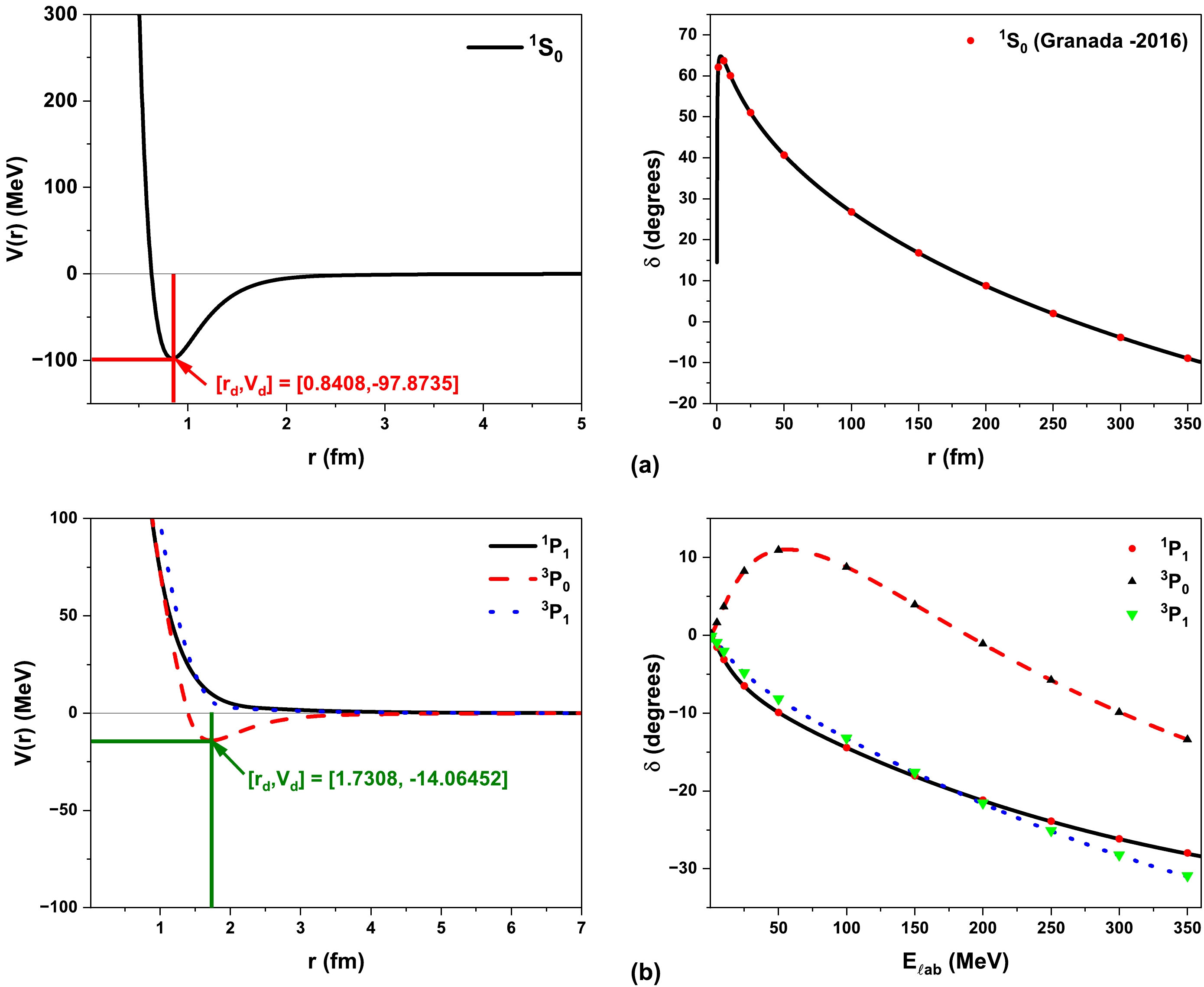
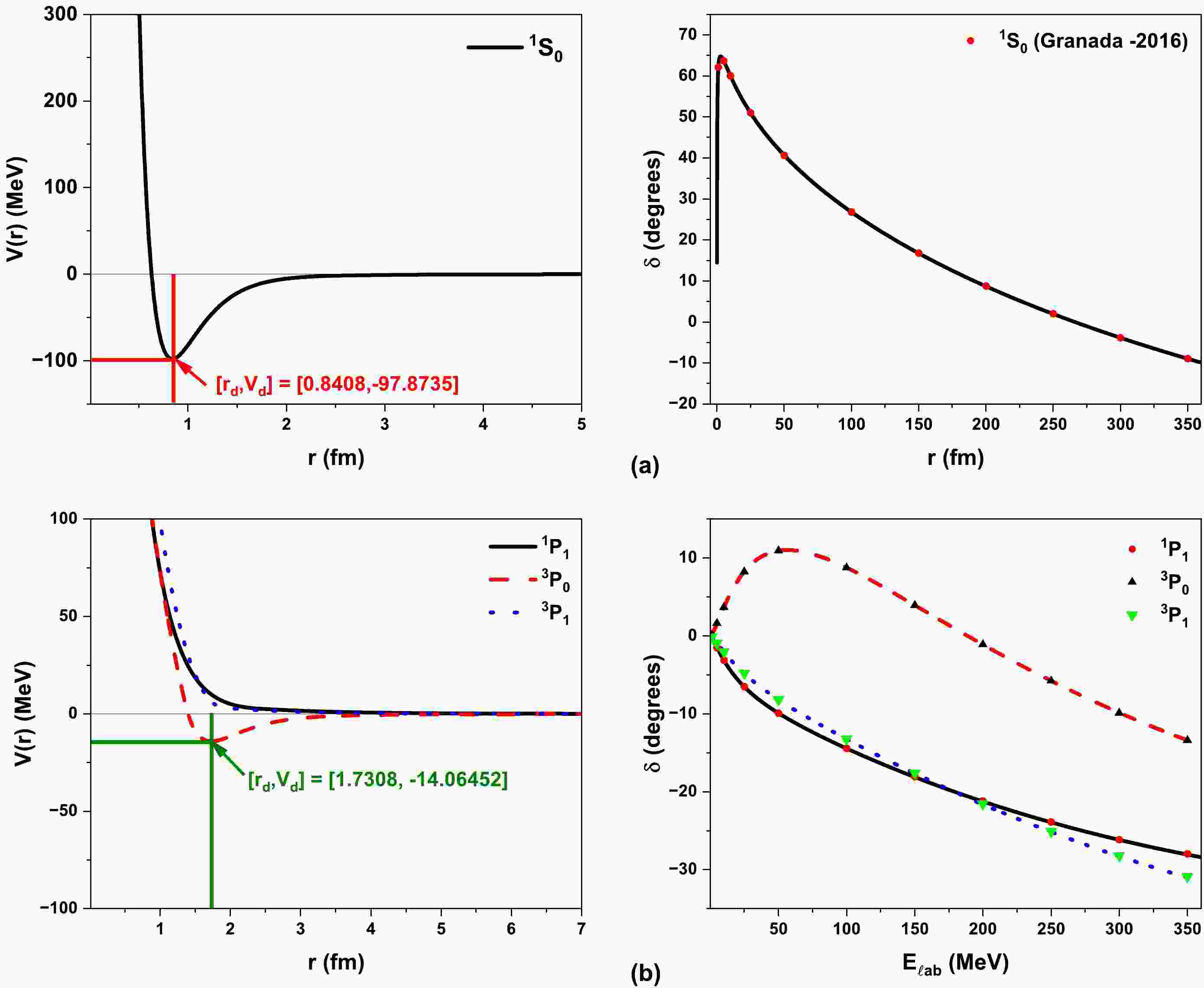
Figure 1.  (color online) Inverse potentials along with scattering phase shifts for the single channel scattering for S and P wave.

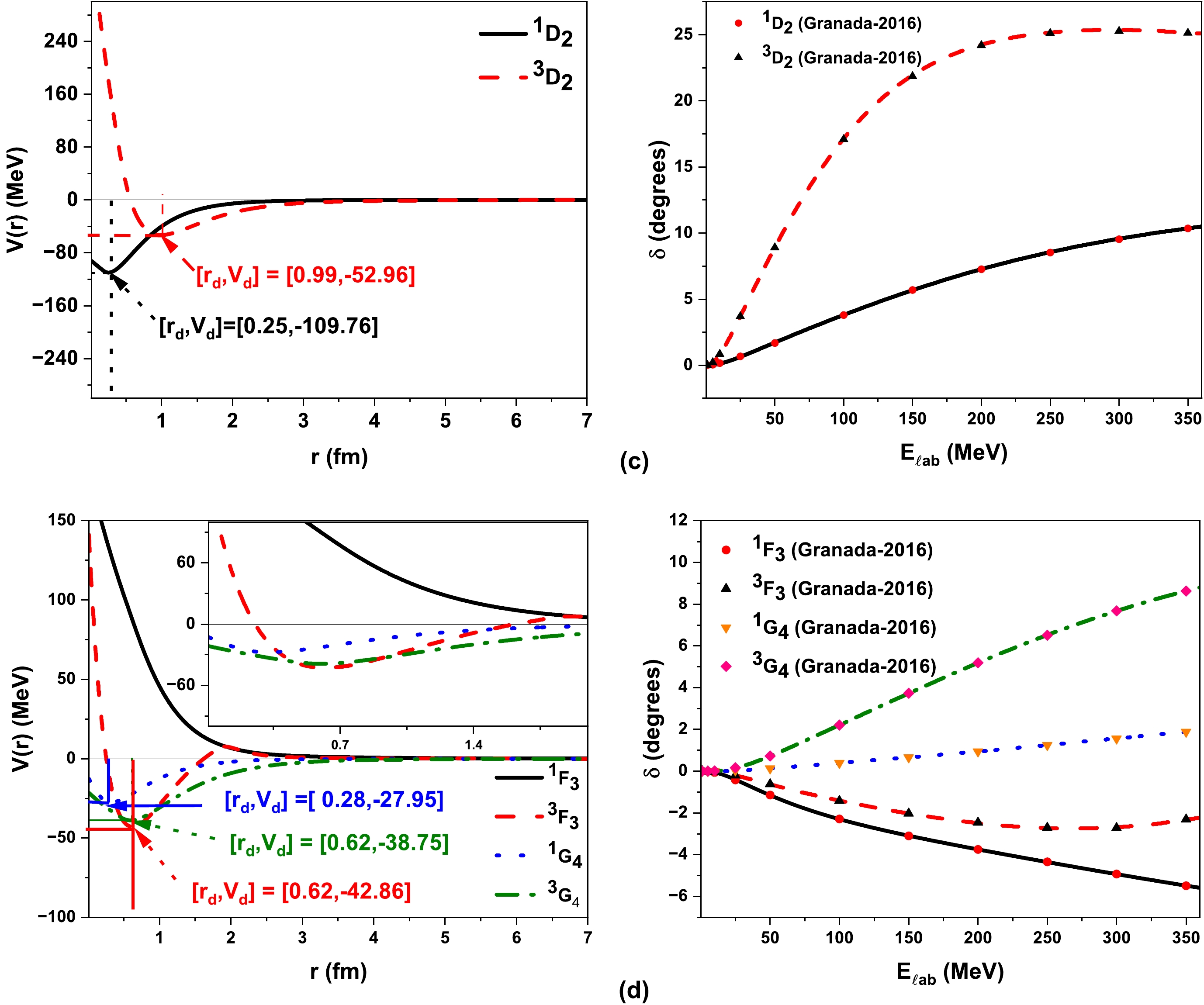
Figure 2.  (color online) Inverse potentials along with scattering phase shifts for the single channel scattering for D, F and G wave.

1. For the $ ^1S_0 $ state, the depth of the potential $ V_d $ is determined to be 97.87 MeV at a distance $ r_d $ of 0.84 fm. Observing the phase shifts depicted in Fig. 1, it's noted that they exhibit a decreasing trend, with positive values from energies of 1 MeV up to 250 MeV. However, from 300 to 350 MeV, the phase shifts are having negative values. This indicates that the constructed inverse potential must manifest an attractive nature for energies up to 250 MeV and strong repulsion at short inter-nuclear distances that can be reached at very high energies. This is seen in Fig. 1(a).

2. For $ \ell = 1 $, there are three states: $ ^1P_1 $, $ ^3P_0 $, and $ ^3P_1 $, each exhibiting single-channel scattering. In the case of the $ ^1P_1 $ and $ ^3P_1 $ states, it's observed that their phase shifts crossover after 200 MeV. Similarly, their respective inverse potentials also crossover at approximately 1.48 fm. For the case of $ ^3P_0 $, phase shifts start from being positive and then cross over to negative values, the repulsive nature of the potential curve can be observed. The depth of potential $ V_d $ is 14.06 MeV at distance $ r_d $ equal to 1.73 fm as shown in Fig. 1(b).

3. For $ \ell = 2 $, there are two single channel states, namely $ ^1D_2 $ and $ ^3D_2 $. For the state $ ^1D_2 $, the phase shifts are consistently positive, indicating an attractive nature. The obtained inverse potentials are purely attractive, with a depth $ V_d $ of 109.76 MeV observed at a distance $ r_d $ of 0.99 fm. Conversely, for the state $ ^3D_2 $, the phase shift values exhibit an increasing trend from 1 MeV to 300 MeV. However, at 350 MeV, the phase shift value decreases, indicating a transition from increasing to decreasing behavior. Consequently, the constructed inverse potentials display both repulsive and attractive characteristics. The depth of potential $ V_d $ is determined to be 52.96 MeV at a distance $ r_d $ of 0.25 fm as shown in Fig. 2(c).

4. For $ \ell = 3 $, $ ^1F_3 $ and $ ^3F_3 $, are single-channel scattering states. For $ ^1F_3 $, the phase shifts are consistently negative, indicating increasing repulsion as the inter-nucleon distances decreases.For $ ^3F_3 $, the phase shifts exhibit a negative trend, initially increasing from 1 MeV to 300 MeV, after which they decrease. This trend resembles a negative parabola. As a result, the obtained inverse potentials encompass both repulsive and attractive components. However, beyond a distance of 1.62 fm, the nature of the potential shifts predominantly towards repulsion, mirroring the change in the nature of the phase shifts. The depth of the obtained potential, denoted as $ V_d $, is measured to be 42.86 MeV at a distance $ r_d $ equal to 0.62 fm, as illustrated in Fig. 2(d).

5. There are two states, namely $ ^1G_4 $ and $ ^3G_4 $, having single channel scattering for $ \ell $ = 4. For both states, the phase shifts are positive and hence the obtained inverse potentials are attractive. For $ ^1G_4 $ and $ ^3G_4 $, the depths $ V_d $ are 27.95 MeV and 38.75 MeV observed at a distance $ r_d $ of 0.28 fm and 0.62 fm respectively as depicted in Fig. 2(d).

In the np system, there exist four channels where the coupling is observed. The degree of this coupling is delineated by the mixing parameters, denoted by $ \epsilon $, which elucidate the interaction between the two states within a specific channel. For many channel scattering, by doing "Stapp Parametrization" [10], we have incorporated the mixing parameter and solved the three coupled non-linear differential equations. From these equations, we have to optimize 30 parameters and construct three inverse potentials corresponding to individual states and their mixing parameters. The potentials corresponding to mixing parameter are the tensor potentials which we get directly on solving the coupled equations. To construct these three potentials simultaneously is a challenge as we have 30 D parameter space. To adjust the bounds of these parameters is a crucial task in the genetic algorithm. To get best optimal solutions, we have adjusted the bounds by solving the single-channel phase equation and get to know where the possible solutions of the equation occurs. So after getting rough idea about the bounds, we have readjusted them to solve the multi-channel scattering equations. To get best possible potentials, we have calculated the MSE of three equations individually and optimized the mean of these MSEs by adjusting their weights. Initially, S, D and mixing have been given equal weightage in determining the mean of their MSE values. It was observed that while S and D channels outputs were closely matching those of mixing channel were not. This is because the phase shift values for S and D channels are significantly larger than those resulting due to their coupling. We have observed that the relative error in phase shifts due to coupling are much higher than those due to individual channels without mixing. Hence, we have doubled the weightage for the MSE obtained for mixing parameters in the formula for mean of MSEs and the results were much improved. So the optimised model parameters for multi-channel scattering are given in the Table 2. The obtained MSEs for these channels are of the order of $ 10^{-2} $. The constructed inverse potentials along with their corresponding phase shifts are depicted in Fig. 3 and Fig. 4. The following observations are made:

States	$ \alpha_{0} $	$ \alpha_{1} $	$ \alpha_{2} $	$ r_{0} $	$ r_{1} $	$ r_{2} $	$ x_1 $	$ x_2 $	$ D_0 $
$ ^3S_1 $	1.7864	3.5192	1.2176	2.2299	0.8673	7.9764	0.0218	1.6569	23.0292
$ \epsilon_1 $	1.0242	2.5235	1.3197	2.0600	0.4000	0.0100	0.0100	2.3578	57.7110
$ ^3D_1 $	0.3691	1.6372	1.0521	3.4736	0.0108	0.0119	0.3218	3.6187	29.1949
$ ^3P_2 $	1.0257	3.1263	1.1437	2.6544	0.5451	4.9708	0.0100	1.4440	23.3281
$ \epsilon_2 $	1.7441	0.3447	0.7514	0.0103	0.4897	14.2702	0.4074	0.5890	93.5844
$ ^3F_2 $	0.6345	0.6979	2.0917	1.6293	0.1262	2.2408	0.5927	1.9031	12.2068
$ ^3D_3 $	0.5912	1.5485	1.6835	1.9402	2.3206	3.0536	0.0956	1.9256	72.7436
$ \epsilon_3 $	0.3993	1.6200	1.0660	1.4897	0.0424	0.0129	0.0141	3.6925	32.5026
$ ^3G_3 $	0.1773	1.5757	1.3185	5.2381	0.5666	1.0581	0.7447	2.6793	19.4466
$ ^3F_4 $	0.9507	2.8765	0.6763	2.1921	1.4048	8.2111	0.8588	3.7172	75.5033
$ \epsilon_4 $	0.6376	1.4582	0.5219	0.0123	1.3187	16.1720	1.0822	4.7992	50.7831
$ ^3H_4 $	0.5228	1.2174	1.8201	0.7222	0.6374	0.2356	0.3636	2.1788	86.7397

Table 2.  Optimised model parameters for channels exhibiting many-channel scattering

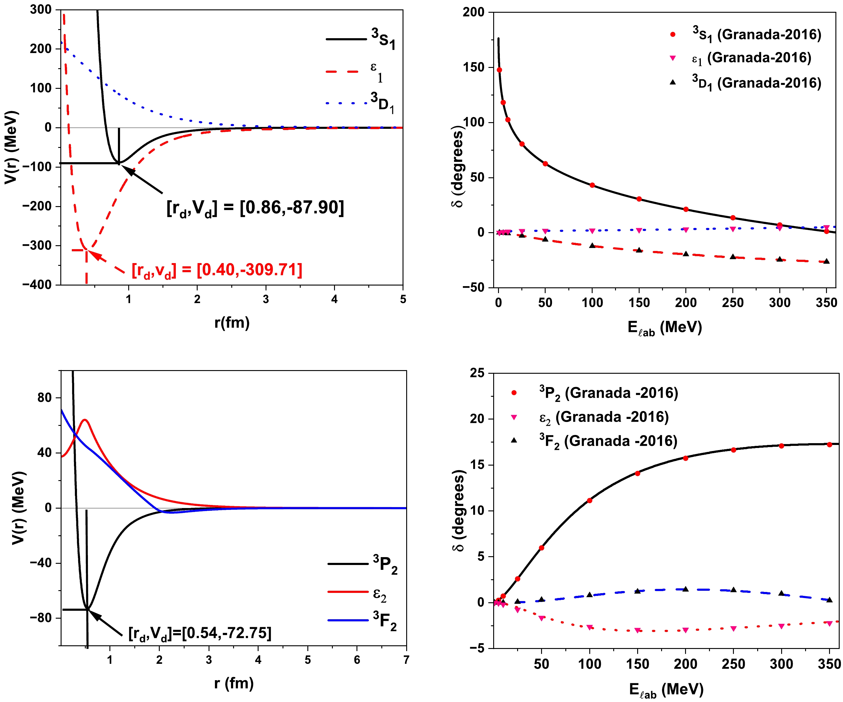
Figure 3.  (color online) Inverse potentials along with scattering phase shifts for the multi channel scattering of J = 1 and 2

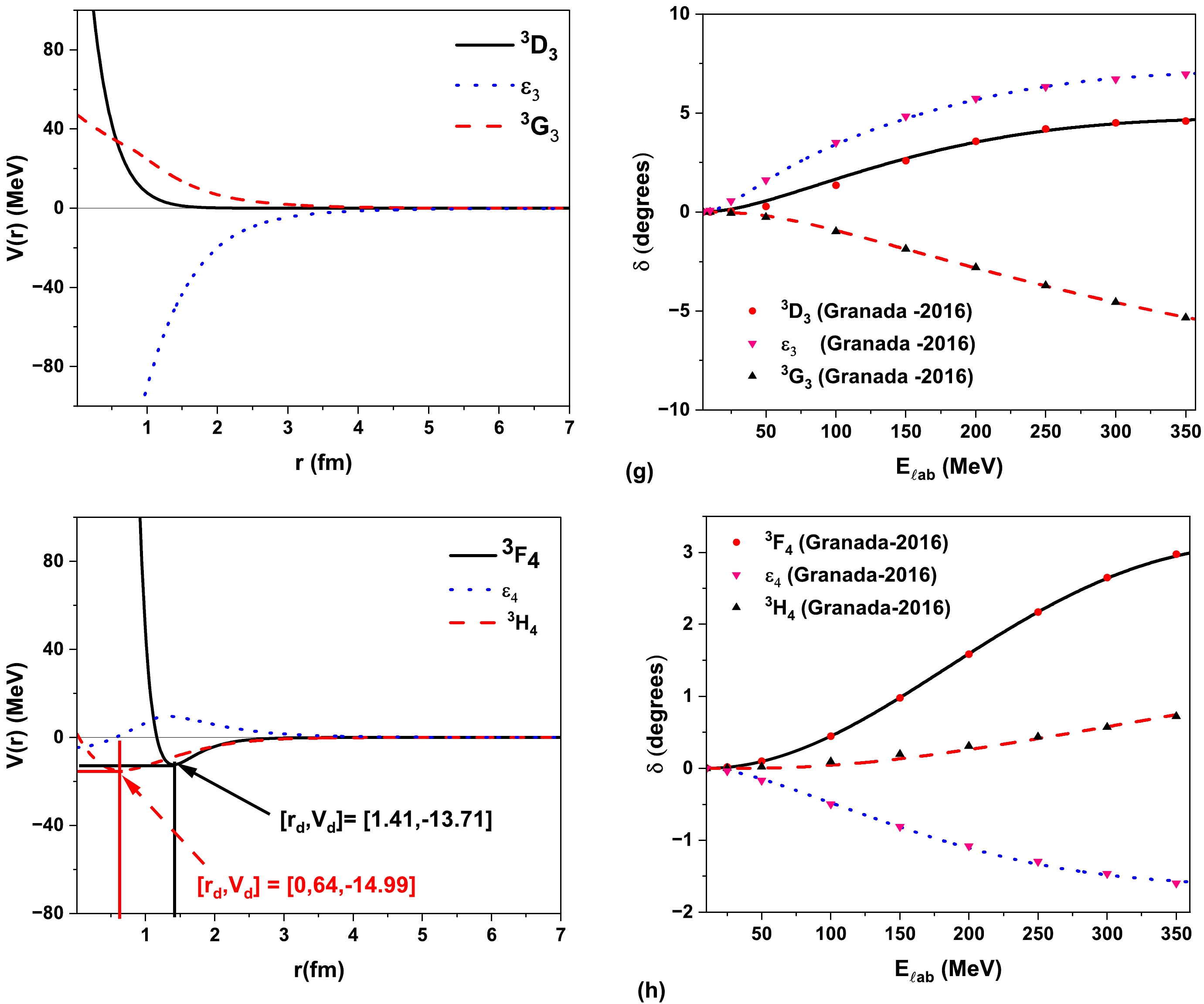
Figure 4.  (color online) Inverse potentials along with scattering phase shifts for the multi channel scattering of J = 3 and 4.

1. For J = 1, there is coupling between $ ^3S_1 $ and $ ^3D_1 $ states. The constructed inverse potentials corresponding to these states are shown in Fig. 3(e). The phase shift values of $ ^3S_1 $ state are in decreasing order and hence exhibit both repulsive and attractive natures having a depth of 87.90 MeV at distance $ r_d $ to be 0.86 fm. The values phase shifts of $ ^3D_1 $ state is negative and hence potential is repulsive in nature. The values of mixing parameter $ \epsilon_1 $ is negative and hence potential is attractive in nature having depth of 309.97 MeV at distance $ r_d $ to be 0.40fm.

2. For J = 2, there is coupling between $ ^3P_2 $ and $ ^3F_2 $ state. The potentials of $ ^3P_2 $ and $ ^3F_2 $ are both repulsive and attractive, with depths $ V_d $ equal to 72.75 MeV and 3.34 MeV at distances $ r_d $ of 0.24fm and 2.24 fm respectively, as depicted in Fig. 3(f). The values of mixing parameter $ \epsilon_2 $ are negative and hence we obtained repulsive interaction as the nature of tensor potential.

3. For $ J = 3 $, there is coupling between $ ^3D_3 $ and $ ^3G_3 $ states. We have a repulsive potential for both $ ^3D_3 $ and $ ^3G_3 $ states. Regarding the mixing parameter $ \epsilon_3 $, the constructed inverse potential is attractive in nature, as depicted in Fig. 4(g).

4. For $ J=4 $, there exists coupling between $ ^3F_4 $ and $ ^3H_4 $ states. In the $ ^3F_4 $ state, the phase shift values increase positively, resulting in an inverse potential exhibiting both repulsive and attractive characteristics, with a depth $ V_d $ of 13.71 MeV at a distance $ r_d $ of 1.41 fm. Conversely, for the $ ^3H_4 $ state, the phase shifts are positive, indicating an attractive nature of the potential, with a depth $ V_d $ of 14.99 MeV at a distance $ r_d $ of 0.64 fm, as illustrated in Fig. 4(h). The mixing parameter $ \epsilon_4 $ takes negative values in increasing order, implying attraction up to 0.64 fm, beyond which repulsion emerges. Consequently, the tensor potential exhibits a more repulsive nature corresponding to $ \epsilon_4 $, as clearly depicted in Fig. 4(h).

Once we obtained the scattering phase shifts, we are now able to calculate the low energy scattering parameters for S state by utilising the effective range approximation formula [35], which is given as:

where k is the centre of mass momentum, $ \delta_0 $ is the phase shift for $ \ell $ = 0, $ a_0 $ is the scattering length, r is the effective range. Using the obtained phase shifts, we have calculated the low energy scattering parameters as given in Table 3. In Table 3, we have compared our results with the most successful high precision potential such as $ Av_{18} $ potential [1] and Granada-2016 [31]. The scattering parameters obtained for the $ ^3S_1 $ state exhibit a remarkable alignment with experimental values, demonstrating a precise match with an error margin of less than 0.6%. For $ ^1S_0 $, the scattering length matches well with the experimental within error of 0.03%, but for effective range there is some discrepancy between our calculations and the experimental results. This seems to be possible because of any possible error in input phase shifts of $ ^1S_0 $. The effective range for $ ^1S_0 $ given by most successful $ Av_{18} $ potential and Granada-2016 is also comes to be 2.69$ fm $ and 2.67$ fm $ respectively.

States	Scattering length '$ a_0 $' (fm)					Effective range 'r' (fm)
	Exp [32]	$ Av_{18} $ [1]	Granada 2016[31]	Our work		Exp [32]	$ Av_{18} $ [1]	Granada 2016[31]	Our work
$ ^1S_0 $	–23.749(8)	–23.732	–23.735	–23.741		2.81(5)	2.697	2.673	2.63
$ ^3S_1 $	5.424(3)	5.419	5.441	5.445		1.760(5)	1.75	1.781	1.770

Table 3.  Low energy scattering parameters of $ ^1S_0 $ and $ ^3S_1 $ state. We have compared our calculations with the realistic potentials like Av-18 [1] and Granada-2016 [31].

Utilising the obtained phase shifts, we have calculated the partial cross-section $ \sigma_{\ell}(E) $ [16, 36] for n-p scattering as:

and thus the total scattering cross section (SCS) $ \sigma_{T} $, [16] is given as

Here 'n' is the number of $ \ell $- channels data available for the scattering system. In our work, we have take n = 5 for all five $ \ell $ channels. The total scattering cross section closely matches the experimental ones [37], as depicted in Fig. 5, within an experimental error of less than 1%. The inset of Fig. 5 represents the contribution of both $ ^1S_0 $ and $ ^3S_1 $ state in the total cross section. One can observe that $ ^1S_0 $ has large contribution at low energies below 1 $ MeV $ and then gradually falls down with increasing energy and becomes very less past 100 $ MeV $. On the other hand, contribution due to the $ ^3S_1 $ state increases beyond 1 $ MeV $ and peaks at 10 $ MeV $ and then falls down. One can also observed that as energy levels increases from 100 $ MeV $ to 350 $ MeV $, the contributions from P and D channels become notably significant, whereas those from F and G states remain comparatively less pronounced within the same range. However, they become increasingly important for accurately representing the observed experimental total SCS. Contributions from the 1 H-state are minimal and have negligible impact on determining the total SCS. Hence, the obtained total scattering cross sections closely align with experimental observations [37].The computed partial and total cross-section values at various energies, alongside experimental values, are compiled in the Table 4.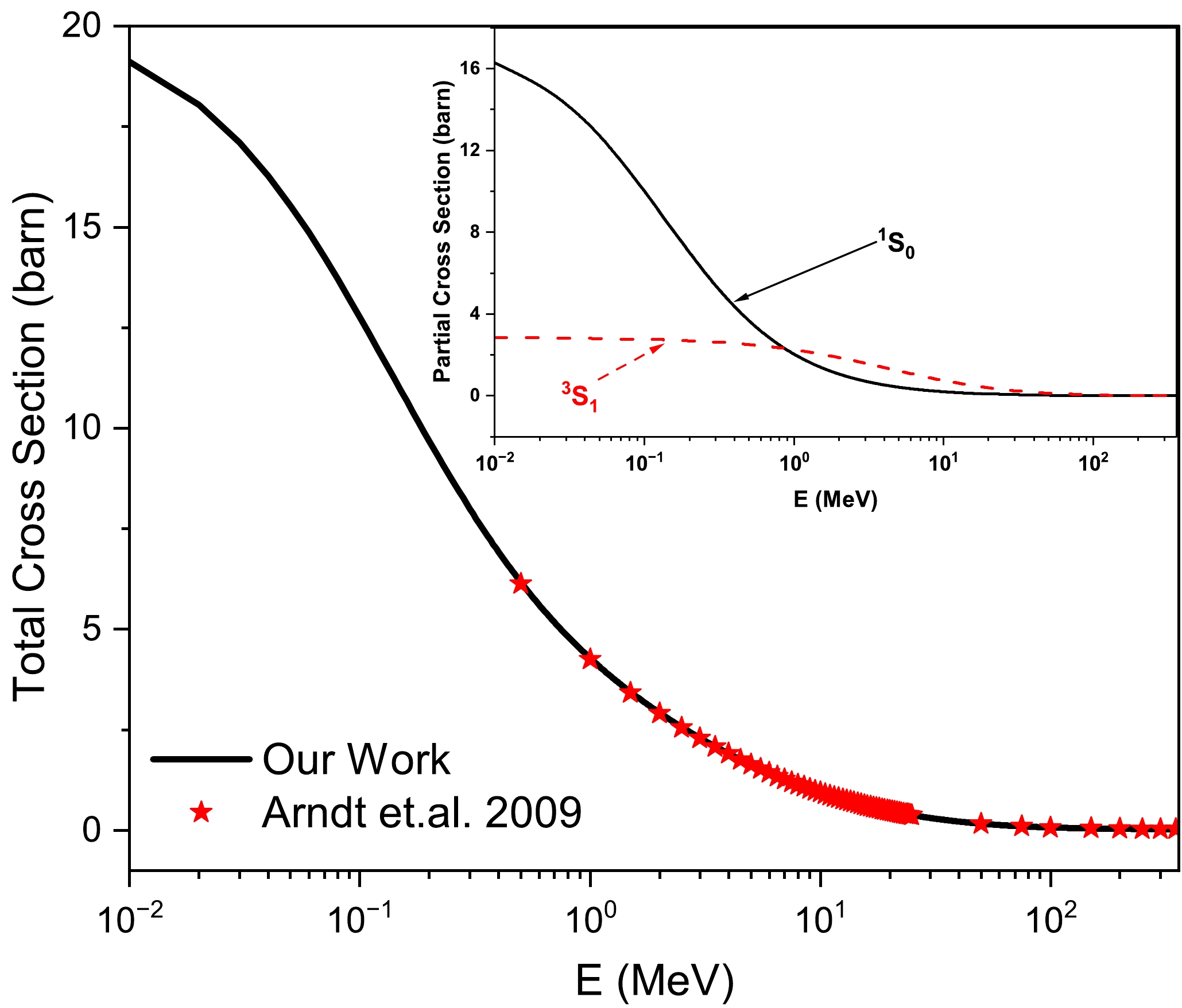

Figure 5.  (color online) The obtained total scattering cross section(SCS) along with experimental SCS [37]. The energy has been plotted on a log scale. Inset shows contributions due to both $ ^1S_0 $ and $ ^3S_1 $ state.

E (MeV)	$ \sigma_{exp} $ [37] (barn)	$ \sigma_{S} $	$ \sigma_{P} $	$ \sigma_{D} $	$ \sigma_{F} $	$ \sigma_G $	$ \sigma_{H} $	$ \sigma_{sim} $ (barn)
1	4.253	4.283 (100%)	0.000	0.000	0.000	0.000	0.000	4.283
5	1.635	1.635 (99.8%)	0.002 (0.2%)	0.000	0.000	0.000	0.000	1.638
10	0.9455	0.9399 (99.3%)	0.0059 (0.6%)	0.0004 (0.1%)	0.0000	0.0000	0.0000	0.9462
25	0.3804	0.3673 (96%)	0.0124 (3.2%)	0.0030 (0.8%)	0.0001	0.0000	0.0000	0.3828
50	0.1684	0.1455 (85.5%)	0.0159 (9.3%)	0.0085 (5%)	0.0002 (0.1%)	0.00000	0.00000	0.1701
100	0.07553	0.04162 (55.1%)	0.01761 (23.3%)	0.01547 (20.5%)	0.00053 (0.7%)	0.00025 (0.3%)	0.00000	0.07549
150	0.05224	0.0148 (28.7%)	0.01837 (35.5%)	0.01734 (33.5%)	0.00069 (1.3%)	0.00052 (1%)	0.00000	0.05175
200	0.04304	0.00534 (12.6%)	0.01883 (44.3%)	0.01678 (39.5%)	0.00073 (1.7%)	0.00079 (1.9%)	0.00000	0.04248
250	0.03835	0.00169 (4.5%)	0.01905 (50.2%)	0.01547 (40.8%)	0.00069 (1.8%)	0.00103 (2.7%)	0.00000	0.03794
300	0.03561	0.00042 (1.2%)	0.01902 (53.8%)	0.01404 (39.7%)	0.00064 (1.8%)	0.00122 (3.4%)	0.00001	0.03535
350	0.03411	0.00019 (0.6%)	0.01878 (55.7%)	0.01270 (37.7%)	0.00066 (2%)	0.00136 (4%)	0.00001	0.0337

Table 4.  The separate contributions of different channels to the overall calculated total elastic scattering cross-section (SCS) are presented. Additionally, the percentage contributions of these channels to the total obtained SCS are indicated in parentheses.

The approach of inverse scattering theory realized computationally through reference potential approach is exactly equivalent to physics informed machine learning paradigm. Instead of adjusting weights in a neural network to obtain the underlying optimization function that best describes the expected data [31], here the parameters of piece-wise smooth Morse function,are varied utilizing Genetic Algorithm [21] to simulate all possible shapes of curves that span a sample space from which one converges to the best model potential. The resultant inverse potentials for various $ \ell $ channels are phenomenological in the sense that they take into account all possible interaction within the scattering particles. The excellent match of our potentials with already existing high precision realistic potentials, based on modeling the various internal interactions, validates our computational approach and hence paves the way for an alternative methodology to understand the inherent nature of interaction in various scattering scenarios. Especially, this reference potential approach leads to a very elegant solution for charged particles scattering [38], where modeling the Coulomb interaction poses a major challenge. In conclusion, we say that our computational methodology to construct inverse potentials based on piece-wise smooth Morse functions as a reference family of curves using a genetic algorithm for optimization has been successful in explaining the experimental outcomes of np-scattering. Our scattering parameters match closely with those obtained by Argonne and Granada researchers. The calculated total cross-sections from the simulated scattering phase shifts are very close to the experimental ones, thus validating our reference potential approach. The constructed potentials can now be utilized to determine the off-shell properties of the deuteron, such as its binding energy and structural electromagnetic form factors. These aspects will be addressed separately. These inverse potentials for various neutron-proton scattering states would be very useful for nuclear ab-initio calculations.

We would like to acknowledge the contributions of Mr. M. G. Ganesh Kumar who has enhanced the efficiency of the code and Dr. Anil Khachi for his preliminary discussions on mixing parameters.

The datasets used and/or analyzed during the current study are available from the Granada Database. https://www.ugr.es/amaro/nndatabase/