


 Abstract
 HTML
HTML Reference
 Related
 PDF
PDF


-
A spallation reaction is one of the violent nuclear reactions, and it occurs when a high-energy light particle strikes a target nucleus. Spallation reactions can naturally occur in the cosmos where high-energy cosmic rays collide with nuclei [1], resulting in the variation of elements in the universe. They can also be artificially induced at a nuclear facility, such as accelerator driven systems (ADS) for nuclear waste disposal, radioactive nucleus production, or during the proton therapy process using accelerated protons. The incident energy in a spallation reaction is above tens of A MeV, which covers the ranges of intermediate energy, relativistic energy, and even higher energies. As a result of the spallation reaction, various radioactive nuclei can be produced, the research regarding which has important applications in several disciplines, including nuclear physics, nuclear astrophysics, isotopic-separation-online (ISOL)-type radioactive-ion-beam facilities, upcoming third-generation radioactive nuclear beams facilities, ADS for nuclear energy [2] and nuclear waste transmutation [3, 4], radioactive nuclei synthesis (especially for extreme nuclei and nuclear isomers [5]), accelerator material radiation [6], and proton therapy [7, 8].
Its extensive applications have attracted both experimental and theoretical interests. In early times, the experiments were usually carried out using accelerated protons on the synchrocyclotron or using cosmic rays. After the reverse kinetic technique was proposed, massive experiments have been performed to measure the spallation fragments above 56Fe, covering the incident energy range of a few hundreds of A MeV to higher than A GeV. Prodigious data for fragments in spallation reactions have been assembled.
On the theoretical front, many models have been developed. The quantum molecular dynamics model has been improved for spallation reactions [9-11]. The statistical multi-fragmentation model [12-14] and the Liège intranuclear cascade (INCL++) model [15-17] (which has been implanted in the OpenMC, GEANT4, and FLUKA toolkits [18, 19]) can be used to simulate spallation reactions, which are usually followed by a secondary decaying simulation to reproduce the experimental results (a review is also recommended [20]). Some semi-empirical parameterizations, including the EPAX [21] and the SPACS [22], can globally predict the residue fragments in the spallation reaction. The nuclear energy agency (NEA) systematically compared the international codes and models for the intermediate energy activation yields to meet the needs of ADS designation, energy amplification, and medical therapy [23]. Difficulties still exist, as the spallation reaction involves a wide incident energy range, as well as a wide range of nuclei, from light to heavy ones. Since the important applications of spallation reactions and the resultant residues productions, it is important to improve the theoretical predictions for the proton induced spallation reactions. The existing models are limited with regard to predicting the light fragments, particularly for proton-induced reactions at low energy. It is necessary to propose a new method for the accurate prediction of the fragments in spallation reactions.
The neural network method, one of the machine learning technologies, is being increasingly employed in nuclear physics. In the standard neural network, it is difficult or even impossible to control the complexity of the model, which is likely to lead to overfitting and reduce the generalization ability of the network [24]. The Bayesian neural network (BNN) provides a good means for avoiding overfitting automatically by defining vague priors for the hyperparameters that determine the model complexity [25]. A prior distribution of the model parameters can be incorporated in Bayesian inference and combined with training data to control the complexity of different parts of the model [26]. Successful examples of BNN applications in nuclear physics can be found in the predictions of nuclear mass [27-29], nuclear charge radii [30], nuclear
$ \beta- $ decay half-life [31], fissile fragments [32], and spallation reactions [33]. Based on the vast numbers of measured fragments in laboratories around the world, it is quite promising to predict spallation cross sections accurately and give reasonable uncertainty evaluations with the BNN approach.In this article, a new method is proposed to predict the fragment cross sections in proton-induced spallation reactions. The BNN method is described in Sec. 2. The results and discussions are presented in Sec. 3, and a conclusion is given in Sec. 4.
-
The key principle of Bayesian learning is to deduce the posterior probability distributions through the prior distribution. The process of Bayesian learning is started by introducing the prior knowledge for model parameters. Based on the given training data
$ D = (x^{(i)},y^{(i)}) $ and model assumptions, the prior distributions for all the model parameters are updated to the posterior distribution using Bayes' rule,$ \begin{array}{l} p(\theta|D) = p(D|\theta)p(\theta)/p(D)\propto L(\theta)p(\theta), \end{array} $

(1) where
$ \theta $ denotes the model parameters. The posterior distribution$ p(\theta|D) $ combines the likelihood function$ p(D|\theta) $ with the prior distribution$ p(\theta) $ , which contains the information about$ \theta $ derived from the observation and the background knowledge, respectively.The introduction of the prior distribution is a crucial step that allows the prediction to go from a likelihood function to a probability distribution. The normalized quantity
$ p(D) $ can be directly understood as the edge distribution of the data, which can be obtained from the integration of the selected model hypothesis and prior distribution$ p(\theta) $ ,$ \begin{array}{l} p(D) = \displaystyle\int_{\theta}p(D|\theta)p(\theta){\rm d}{\theta}. \end{array} $

(2) In this work, the prior distributions
$ p(\theta) $ are set as the Gaussian distributions. The precisions (inverse of variances) of these Gaussian distributions are set as gamma distributions [28], which automatically control the complexity of different parts of the model. The likelihood function$ p(D|\theta) $ and the objective function$ \chi^{2}(\theta) $ are given by$ \begin{split}& p(D|\theta) = {\rm exp}(-\chi^{2}/2), \ \ \chi^{2} = \sum\limits_{i}^{N} [y_{i}-f(x_{i};\theta)]^2 / \Delta{y_{i}^2}, \end{split} $

where
$ \Delta{y_{i}^2} $ is the associated noise scale. The function$ f(x, \theta) $ is a multilayer perceptron (MLP) network, which is also known as the "back-propagation" or "feed-forward." A typical MLP network consists of a set of input variables ($ x_{i} $ ), certain hidden layers, and one or more outputs ($ f_{k}(x; \theta) $ ). For an MLP network with one hidden layer and one output, the function is defined as$ \begin{array}{l} f(x;\theta) = a+\displaystyle\sum\limits_{j = 1}^{H}b_j\, {\rm tanh}\left(c_j+\displaystyle\sum\limits_{i = 1}^{I} d_{ji} x_i\right), \end{array} $

(3) where H denotes the number of hidden units, and I is the number of input variables.
$ \theta = (d_{ji}, c_{j}) $ and$ \theta = (b_{j}, a) $ are the weights and bias of the hidden layers and output layer, respectively.Based on the theoretical principles and prior knowledge, the posterior distribution can be obtained from the data using Eq. (1). The predictive distribution of output
$ y^{\rm new} $ for a new input$ x^{\rm new} $ is obtained by integrating the predictions of the model with respect to the posterior distribution of the model parameters,$ \begin{array}{l} p(y^{\rm new}|x^{\rm new},D) = \displaystyle\int p(y^{\rm new}|x^{\rm new},\theta) p(\theta){\rm d}\theta. \end{array} $

(4) In the MLP network, we are interested in obtaining a reasonable prediction with the new input
$ x^{\rm new} $ rather than the posterior distribution for parameters. For a new input$ x^{\rm new} $ , the model prediction$ y^{\rm new} $ can be obtained from the mathematical expectation of the posterior distribution,$ \begin{array}{l} y^{\rm new} = E[y^{\rm new}|x^{\rm new},D] = \displaystyle\int f(x^{\rm new},\theta) p(\theta|D){\rm d}\theta. \end{array} $

(5) The integral of Eq. (5) is complex, and a numerical approximation algorithm will reduce the complexity. The Markov chain Monte Carlo (MCMC) methods are applied to optimize the model control parameters and obtain the predictive distribution. As one of the MCMC methods, the hybrid Monte Carlo (HMC) algorithm was first introduced by Neal [34] to deal with the model parameters and Gibbs sampling for hyperparameters. The HMC is a form of the metropolis algorithm, where the candidate states are found via dynamical simulation. It makes effective use of gradient information to reduce the random walk behavior. In theory, the Gibbs sampler is the simplest Markov chain sampling method, which is also known as the heatbath algorithm. The hyperparameters are updated separately using Gibbs sampling, which allows their values to be used in obtaining good step-sizes for the discretized dynamics, and they help to minimize the amount of tuning needed for a good performance in HMC. The integral of Eq. (5) is approximately calculated as
$ \begin{array}{l} y^{\rm new} = 1/K\displaystyle\sum\limits^{K}_{k = 1}f(x^{\rm new},\theta^{t}), \end{array} $

(6) where K is the number of iteration samples. In a previous work, the BNN approach has been adopted to learn and predict the cross sections directly [33]. To provide some physical guidelines, a recent empirical parameterization for fragment prediction, which is named as the SPACS [22], has been adopted for spallation reactions to obtain the fragment cross sections. In this work, the BNN approach is employed to reconstruct the residues between the experimental data (
$ \sigma^{\rm exp} $ ) and the theoretical predictions ($ \sigma^{\rm th} $ ), i.e.,$ \begin{array}{l} y_{i} = \rm{lg}(\sigma^{\rm exp})-\rm{lg}(\sigma^{\rm th}). \end{array} $

(7) The cross section predictions via the BNN approach are then given as
$ \begin{array}{l} \sigma^{\rm BNN+th} = \sigma^{\rm th}\times10^{y^{\rm new}}, \end{array} $

(8) where
$ \sigma^{\rm th} $ and$ y^{\rm new} $ denote the SPACS results and the BNN predictions, respectively. In this work,$ \sigma^{\rm th} $ refers to the predictions obtained using the SPACS parameterizations; As mentioned earlier, the SPACS was proposed recently and has gained success with regard to spallation reactions.The inputs of the neural network are the mass numbers
$ A_{pi} $ ($ A_{i} $ ), the charge numbers$ Z_{pi} $ ($ Z_{i} $ ) of the projectile (fragment) nucleus, and the bombarding energy (in MeV/u)$ E_{i} $ , i.e.,$ x_{i} = (A_{pi}, Z_{pi}, E_{i}, Z_{i}, A_{i}) $ . Systematic experiments have been performed at the Lawernce Berkeley Laboratory (LBL), RI Beam Facility (RIBF) RIKEN, and FRagment Separator (FRS) GSI, which cover a broad range of spallation nuclei, from 36Ar to 238U. The range of the incident energy varied from 168 MeV/u to 1500 MeV/u, which is relevant for the ADS and proton therapy applications. As listed in Table 1, 3511 datasets from 20 different reactions will be used in this work. The complete data are divided into two different sets, which serve as the learning set and the validation set, respectively. The learning set is built by randomly selecting 3211 datasets, and the remaining 300 datasets are selected as the validation set.$ ^{A}{\rm X} $ + p

E/(MeV/u) numbers $ Z_{i} $ 

Ref. 36Ar + p 361 42 9-17 [35] 546 42 9-17 765 38 9-17 40Ar + p 352 45 9-17 [35] 40Ca + p 356 48 10-20 [36] 565 54 10-20 763 54 10-20 56Fe + p 300 128 10-27 [37] 500 136 10-27 750 148 8-27 1000 152 8-26 1500 157 8-27 136Xe + p 168 73 48-55 [38] 200 96 48-55 [39] 500 271 41-56 [40] 1000 604 3-56 [41] 197Au + p 800 352 60-80 [42] 208Pb + p 500 249 69-83 [43] 1000 458 61-82 [44] 238U + p 1000 364 74-92 [45] Table 1. A list of the adopted data for the measured fragments in the X + p spallation reactions.
-
The network is trained with different model structures, and 2000 iteration samples are taken in each training. Because the fragment cross sections may differ by several orders of magnitude, an A-factors method [46, 47] is introduced to indicate the validation results of different models, as shown in Fig. 1. The A-factor is defined as
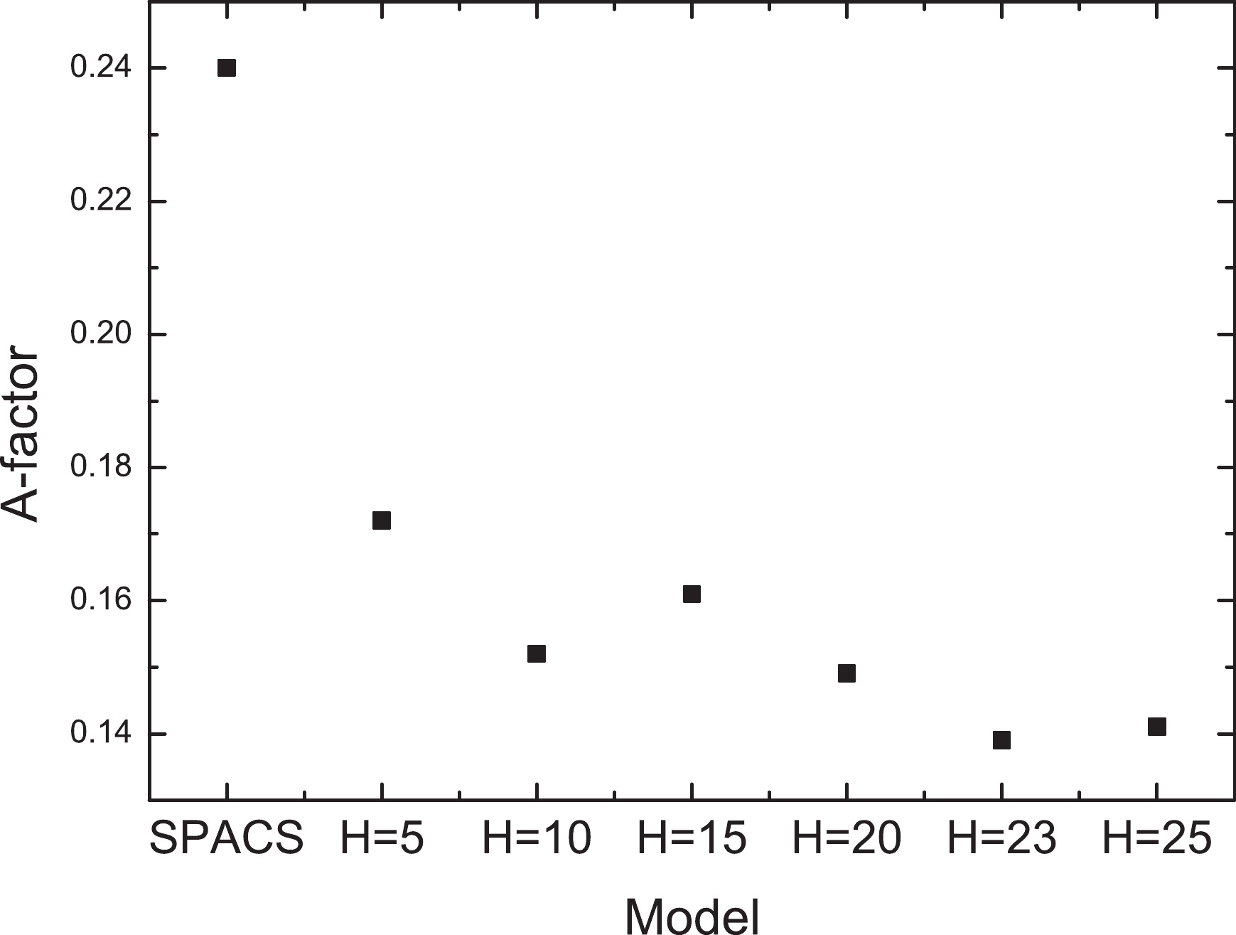
Figure 1. A-factor for the predictions by the SPACS and the BNN + SPACS model with different numbers of hidden neurons, denoted by H, for the validation set.
$ \begin{array}{l} A_f = 1/N\displaystyle\sum\limits^{N}_{i = 1}\frac{|\sigma^{\rm exp} - \sigma^{\rm pre}|}{\sigma^{\rm exp} + \sigma^{\rm pre}}, \end{array} $

(9) where
$ \sigma^{\rm exp} $ and$ \sigma^{\rm pre} $ denote the measured data and the predicted data, respectively. In the following section, we discuss the predictions obtained using the BNN + SPACS method, and compare them with the measured data and the SPACS predictions.In Fig. 1, the A-factors for the SPACS predictions and BNN method with different numbers of hidden neurons are compared. It is observed that even the BNN with five hidden neurons can significantly improve the predictions. The A-factor decreased with an increase in H. When H increased to 23, the A-factor could not be minimized further. A 5-23-1 structure is taken as the optimal network structure, which means that 5 inputs
$ x_{i} = (A_{pi}, Z_{pi}, E_{i}, Z_{i}, A_{i}) $ , 1 output$ y_{i} = \rm{lg}(\sigma^{\rm exp})-\rm{lg}(\sigma^{\rm th}) $ , and a single hidden layer with 23 hidden neurons are included.The BNN + SPACS predictions for fragment cross sections in the 1 A GeV 136Xe + p, 168 A MeV 136Xe + p, 356 A MeV 40Ca + p, and 1 A GeV 238U + p reactions are shown in Fig. 2 to Fig. 5, and compared with the experimental data as well as the SPACS predictions.
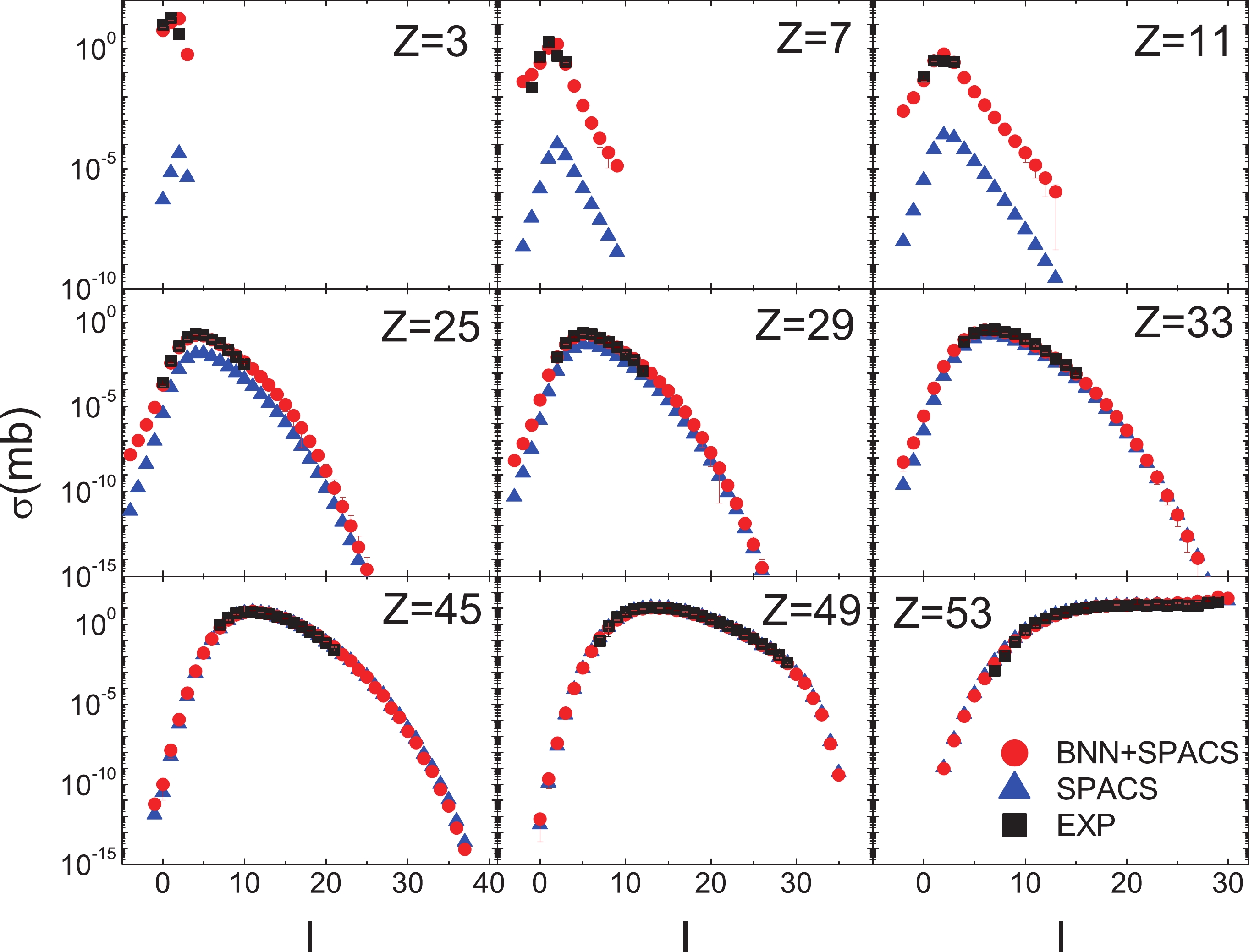
Figure 2. (color online) BNN + SPACS predictions of fragment cross sections of 1000 A MeV 136Xe + p compared with SPACS and experimental data (taken from [41]). In the x axis, I = N - Z denotes the fragment neutron excess. The measured data, BNN + SPACS predictions, and SPACS predictions are plotted as squares, circles, and triangles, respectively. The experimental and BNN + SPACS error bars are too small to be shown.
In Fig. 2, the predicted and measured fragment cross sections in the 1 A GeV 136Xe + p reaction are compared. It is observed that the BNN + SPACS predictions agree quite well with the measured data for fragments from
$ Z = $ 3 to 54. For the fragments with$ Z \leqslant $ 25, the underestimation of experimental data by SPACS has been improved significantly.Figure 3 shows the BNN + SPACS predictions for fragment cross sections in the 168 A MeV 136Xe + p reaction, which have been measured at RIBF, RIKEN recently [38]. In [38], only the cross sections for
$ Z \geqslant $ 48 fragments were reported. Compared to the measured fragments, the BNN + SPACS predictions are very close to the SPACS ones. For the light and medium fragments ($ Z \leqslant $ 25), the BNN + SPACS predictions are substantially higher than the SPACS ones, which are similar to the results shown in Fig. 2. In addition, the uncertainties are relatively large for the$ Z \leqslant $ 11 isotopes. This may be caused by the insufficient data in the training set for this incident energy.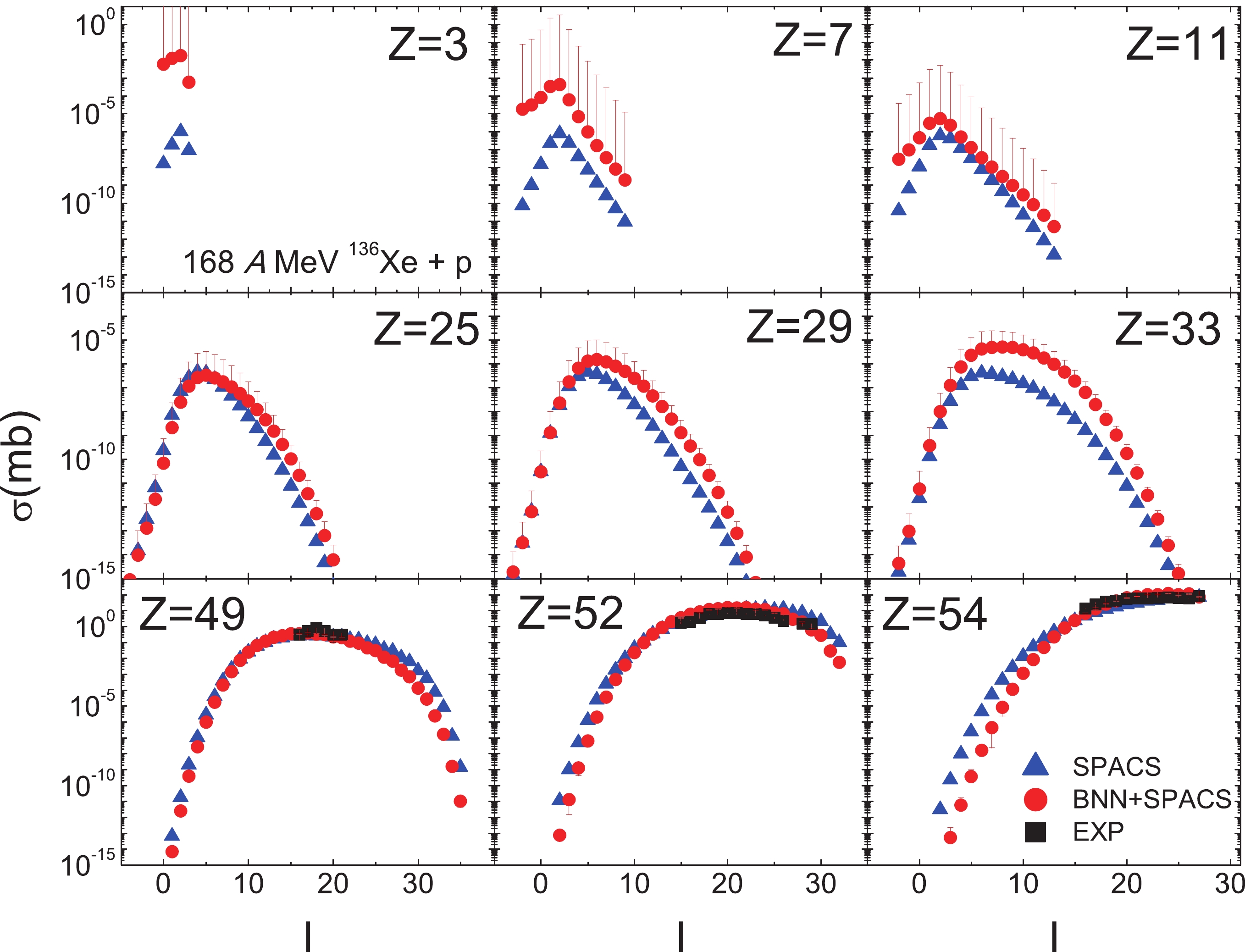
The spallation of intermediate nuclei is of interest in proton therapy and nuclear astrophysics. The composition of interstellar matter is influenced by cosmic ray (mainly high-energy proton)-induced spallation reactions. The 40Ca + p reaction at 356 A MeV, for which the predicted and measured results are shown in Fig. 4, has been studied. Compared to the measured results, both the BNN + SPACS and SPACS predictions could reproduce the experimental data quite well. The fragment cross sections predicted by the BNN + SPACS method are in line with those predicted by SPACS except for the
$ Z = $ 3 isotopes.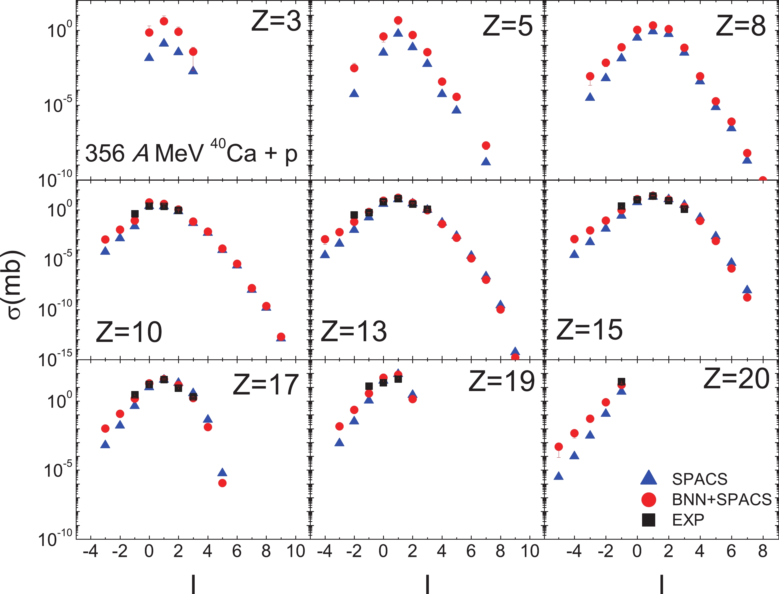
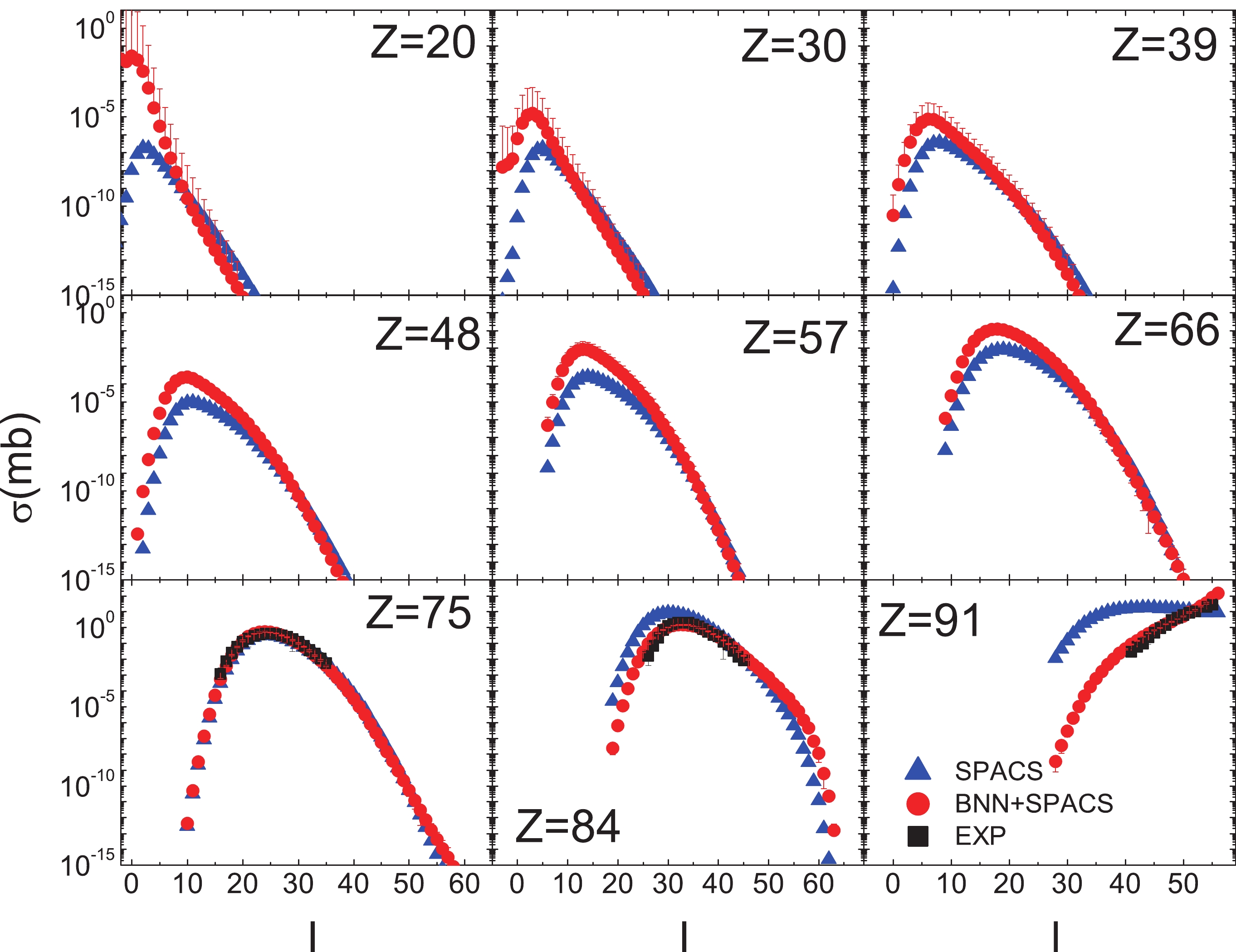
The predictions for the fragment cross sections in the 1 A GeV 238U + p reaction are compared in Fig. 5. The measured data cover the fragments from
$ Z = $ 74 to 92 [45]. It can be observed that the BNN + SPACS method can predict the results well, while the SPACS highly overestimated the measured results for$ Z = $ 91. The BNN + SPACS method shows the sign of larger than the SPACS method for the fragments of smaller I. It seems that for the$ Z = $ 20 isotopes, for fragments from the spallation of a heavy system such as 238U, the predictions by BNN + SPACS become more inaccurate, which indicates that the BNN should be further improved by incorporating more data for small Z fragments produced in the heavy systems.The BNN + SPACS predictions are further verified by using the correlation between the cross section and the average binding energy, which has been elucidated in Ref. [33]. It is generally believed that the isotopic cross section depends on the average binding energy in the form of
$ \sigma = C \rm{e}^{(B'-8)/\tau} $ , where C and$ \tau $ are free parameters, and$ {B' = (B-\epsilon_{p})/A} $ (in which$ \epsilon_{p} = 0.5[(-1)^{N}+ (-1)^{Z}]\epsilon_{0} A^{-3/4} $ is the pairing energy for the fragment, and$ \epsilon_{0} = $ 30 MeV). It is evident that the isotopic cross sections predicted by the BNN + SPACS model for$ Z = $ 17 and 41 obey the correlation very well, which improves both the previous BNN method and also the SPACS method Fig. 6.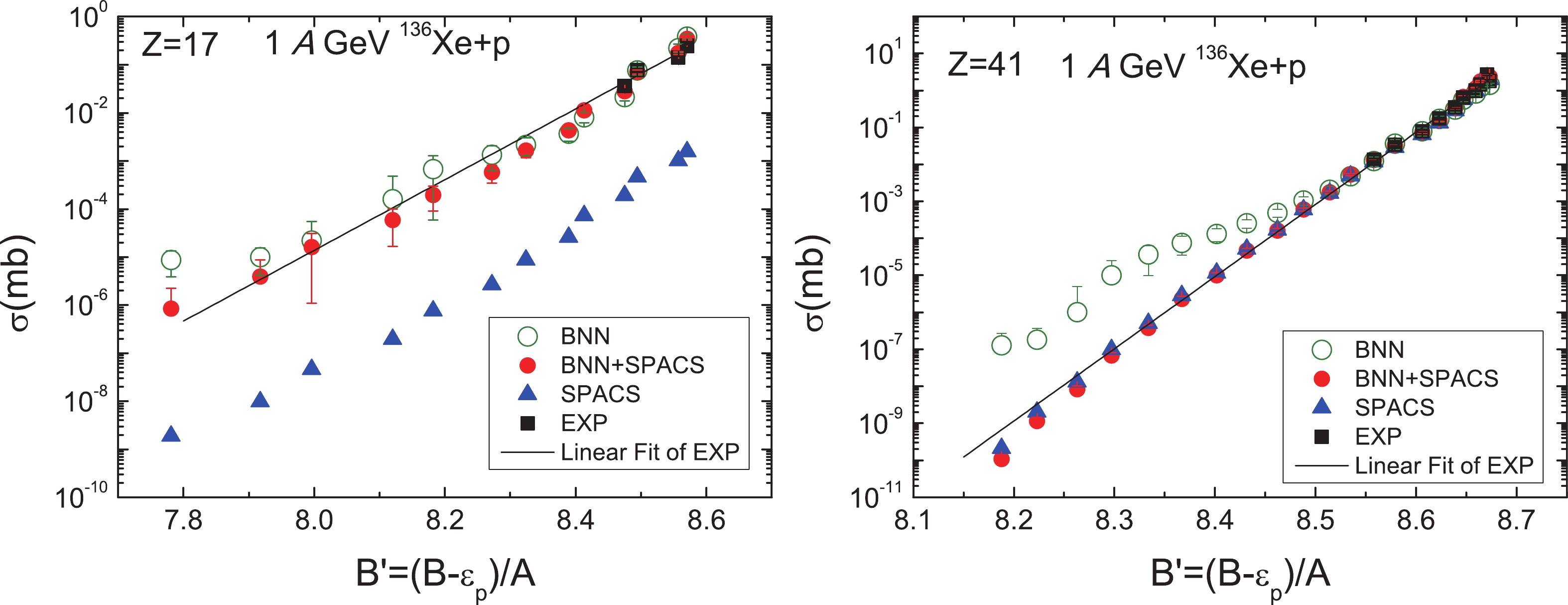
Figure 6. (color online) Isotopic cross section dependence on average binding energy for fragments of Z = 17 and 41 produced in the 1 A GeV 136Xe + p reaction (experimental data taken from [41]). The open circles, solid circles, triangles, and squares denote the data corresponding to the BNN predictions (see Ref. [33]), BNN + SPACS in this work, SPACS, and the measured data, respectively. The solid line denotes the fitting to the experimental data (see text for further explanation).
From the above results, which cover the fragment cross section predictions for proton-induced reactions ranging from intermediate to heavy nuclei and for the incident energy range of 168 A MeV to 1 A GeV, it is observed that the BNN approach improves the quality of the empirical SPACS parameterizations through the reconstruction of the residual cross sections between the SPACS predictions and measured data. Thus, the BNN + SPACS method can be a new tool to predict the fragment cross section in spallation reactions since it can work independently after the network is formed.
If we revisit the foundation of the BNN approach, it is natural that the BNN + SPACS model should provide a better prediction than the SPACS parameterizations since the difference between the SPACS and measured data has been minimized. Therefore, the BNN + SPACS model makes improved predictions and also avoids the nonphysical phenomenon by forming a direct BNN learning network from the measured data, as shown in Ref. [33]. The physical implantations of SPACS play important roles to make the BNN + SPACS method reasonable in physics, and the learning and predicting abilities of the BNN also improve the predictions where the SPACS parameterizations do not perform well.
The results indicate that the SPACS tends to underestimate the cross sections for fragments with relatively small Z, whereas it overestimates the cross sections for fragments with Z close to those for heavy spallation nuclei. These shortcomings have been overcome by the BNN + SPACS model. Limitations still exist for the BNN + SPACS model constructed in this work due to the absence of experimental data for reactions of incident energy below 100 A MeV and for small spallation systems. For applications in proton therapy, the incident energy can be lower than 100 A MeV, and the masses of the spallation nuclei are smaller than 30. The smallest spallation reaction adopted in this work is for 36Ar. If we consider interstellar matter, most of the nuclei have mass numbers smaller than 56. Regarding the spallation reactions induced by high-energy cosmic rays and the proton therapy process, we should improve the prediction model to account for small spallation systems, for which the SPACS parameterizations do not work well. It is important to improve the BNN + SPACS predictions by introducing new data for spallation reactions of intermediate energy (for example, below 100 A MeV) and intermediate/small systems (
$ A < $ 20), which requires new experiments. -
In this article, the BNN approach combined with the SPACS parameterizations is proposed to predict the fragment cross sections in proton-induced spallation reactions. Based on 3511 measured fragment cross sections corresponding to 20 spallation reaction systems, the optimal network structure has been established to be 5-23-1, which includes 5 inputs, 1 output, and a single hidden layer with 23 hidden neurons. By reconstructing the residuals between the measured data and the SPACS predictions, the BNN + SPACS method is verified to well reproduce the experimental data. It is also shown that the BNN + SPACS method can yield a better global prediction compared to the SPACS parameterizations. The established BNN + SPACS method can be potentially applied for research on nuclear physics, nuclear astrophysics, ADS, proton therapy, etc.
A Bayesian-neural-network prediction for fragment production in proton induced spallation reaction
- Received Date: 2020-04-06
- Accepted Date: 2020-07-15
- Available Online: 2020-12-01
Abstract: Fragment production in spallation reactions yields key infrastructure data for various applications. Based on the empirical SPACS parameterizations, a Bayesian-neural-network (BNN) approach is established to predict the fragment cross sections in proton-induced spallation reactions. A systematic investigation has been performed for the measured proton-induced spallation reactions of systems ranging from intermediate to heavy nuclei systems and incident energies ranging from 168 MeV/u to 1500 MeV/u. By learning the residuals between the experimental measurements and SPACS predictions, it is found that the BNN-predicted results are in good agreement with the measured results. The established method is suggested to benefit the related research on nuclear astrophysics, nuclear radioactive beam sources, accelerator driven systems, proton therapy, etc.


 DownLoad: