Minimal lepton models with non-holomorphic modular A₄ symmetry

The Standard Model (SM) successfully describes particle interactions but leaves unexplained the origin of fermion families and their highly hierarchical masses and mixing patterns—a challenge known as the flavor problem [1]. The masses of fundamental particles span more than twelve orders of magnitude, ranging from the neutrino mass on the order of a fraction of an eV to the top quark mass of 173 GeV. Moreover, the quark mixing angles are small, whereas the lepton mixing angles consist of two large angles and one small angle comparable in magnitude to the Cabibbo angle [1]. The SM attributes these patterns to arbitrary Yukawa couplings, providing no underlying principle for their observed hierarchy and structure.

Several approaches have been developed to address the flavor problem. One line of research introduces flavor symmetries, particularly non-Abelian discrete groups such as $ A_{4} $, $ S_{4} $ and $ A_{5} $ which can naturally reproduce large lepton mixing [2−12]. In this framework, the spontaneous breaking of such a family symmetry by scalar flavon VEVs gives rise to the vacuum alignment problem. This introduces additional complications. Modular invariance addresses these issues by offering an economical framework in which Yukawa couplings are modular forms transforming as irreducible representations of the finite modular groups $ \Gamma_{N} $ or $ \Gamma^{\prime}_{N} $, thereby eliminating flavons and removing the need for vacuum alignment [13−15]. This approach enables highly predictive fermion mass models. In the minimal modular invariant model, all lepton masses and mixing parameters are determined by only four real parameters plus the modulus τ [16, 17]. The same modulus can also link quark and lepton sectors, allowing a simultaneous description of their flavor observables with just fourteen real parameters, including the real and imaginary parts of τ [17, 18]. However, the predictive power of this framework is limited because modular symmetry only weakly constrains the K$ \ddot{\mathrm{a}} $hler potential [19]. Integrating modular symmetry with a traditional flavor symmetry resolves this limitation and gives rise to either an eclectic flavor group [20−28] or quasi-eclectic flavor symmetry [29].

In the framework of the original modular invariance approach, the Yukawa couplings are assumed to be modular forms of level N which are holomorphic functions of the complex modulus τ. To preserve this holomorphicity, supersymmetry (SUSY) is required [13, 30−32]. However, experimental evidence for low-energy SUSY remains elusive, making its natural realization uncertain. This motivates the study of non-supersymmetric modular invariant theories. Recently, a non-holomorphic modular flavor symmetry framework has been developed, which remains valid in non-supersymmetric settings [33]. In this framework, the holomorphicity condition is replaced by a harmonic one, and the Yukawa couplings are required to be polyharmonic Maaß forms of level N and even weight. These forms can be decomposed into multiplets of the inhomogeneous finite modular group $ \Gamma_{N} $. Unlike holomorphic modular forms, which are defined only for non-negative weights $ k\geq0 $, the polyharmonic Maaß forms extend to negative weights. Moreover, non-holomorphic polyharmonic Maaß exist for weights $ k = 0,1 $ and $ 2 $. Phenomenologically viable models based on finite modular groups such as $ \Gamma_2\cong S_3 $ [34], $ \Gamma_3\cong A_4 $ [33, 35−47], $ \Gamma_4\cong S_4 $ [48], and $ \Gamma_5\cong A_5 $ [49] have been successfully constructed. The framework has further been extended to include odd-weight polyharmonic Maaß forms, which transform under irreducible representations of the homogeneous finite modular groups $ \Gamma^{\prime}_{N} $ [50]. Modular invariant models based on the corresponding non-holomorphic groups $ \Gamma^{\prime}_{3}\cong T^{\prime} $ [50] and $ \Gamma^{\prime}_{5}\cong A^{\prime}_{5} $ [51] have also been studied. Furthermore, the non-holomorphic modular symmetry can consistently combine with generalized CP (gCP) symmetry, which restricts the phases of couplings, boosting modular invariant model predictions, as in supersymmetric modular flavor symmetry [52]. Under modular transformations, the gCP operation acts as $ \tau \stackrel{{\rm{CP}}}{\longmapsto} -\tau^* $ [20, 21, 52−54]. In the basis where S and T are unitary and symmetric across all irreducible representations, the gCP transformation simplifies to conventional CP, represented by the identity in flavor space.

This work provides a systematic analysis of lepton models based on non-holomorphic $ A_{4} $ modular symmetry. We focus on the most economical modular invariant constructions, which require no flavon fields other than the modulus τ and generate light neutrino masses through the Weinberg operator. The three generations of left-handed leptons are assigned to the irreducible triplet representation 3 of $ A_{4} $, while the right-handed leptons are allowed to transform as all possible combinations of the singlet representations 1, $ {{\bf{1}}^{\bf{\prime}}} $ and $ {{\bf{1}}^{{\bf{\prime\prime}} }}$. Using the level 3 polyharmonic Maaß forms of weights $ k = \pm4,\, \pm2,\, 0 $, we construct all phenomenologically viable and minimally parameterised lepton models. Without imposing gCP symmetry, 147 models for normal ordering (NO) and 6 models for inverted ordering (IO) successfully reproduce the experimental data. When gCP symmetry is enforced, 47 of the 147 NO models and 5 of the 6 IO models remain consistent with the observations in the lepton sector. The current JUNO [55] constraint on $ \sin^{2}\theta_{12} $ rules out only 5 of the 147 viable NO models without gCP symmetry. All others remain consistent with current measurements. Notably, the non-holomorphic $ A_4 $ modular symmetry yields a richer set of level 3 polyharmonic Maaß forms than its supersymmetric framework [56]. This expanded landscape allows the construction of more viable minimal lepton models consistent with experimental data.

We organise the rest of this paper in the following. In section 2, we present a class of minimal lepton flavor models invariant under the non-holomorphic $ A_4 $ modular symmetry, and examines their predictions for lepton mixing angles, CP-violating phases and neutrino masses. A representative model is introduced in section 3, where a detailed numerical analysis is performed for both NO and IO neutrino mass spectra. We conclude the paper in section 4.

In this section, we systematically classify the minimal lepton mass models based on finite modular symmetry $ \Gamma_{3}\cong A_{4} $ in the framework of non-supersymmetry. The Yukawa couplings are described by the polyharmonic Maaß forms of level $ N = 3 $ and even weights, which can be decomposed into the irreducible multiplets of $ A_{4} $. The polyharmonic Maaß form multiplets of level 3 and weights $ \pm 4 $, $ \pm2 $ and $ 0 $ are listed in table 1. The explicit expressions for these forms are omitted here due to their length, and they can be found in Ref. [33].

The finite modular group $ A_{4} $ is generated by the modular transformations S and T, subject to the relations:

where the generators S and T in the three one-dimensional irreducible representations 1, $ {{\bf{1}}^{\bf{\prime}}} $, $ {{\bf{1}}^{{\bf{\prime\prime}} }}$, and one three-dimensional irreducible representation 3 are taken to be:

with $ \omega = e^{2\pi i/3} $. For any two triplets $ x = (x_{1},x_{2},x_{3}) $ and $ y = (y_{1},y_{2},y_{3}) $, the tensor product decomposition $ {\bf{3}}\otimes{\bf{3}} = {\bf{1}}\oplus{{\bf{1}}^{\bf{\prime}}}\oplus{{\bf{1}}^{\prime\prime}}\oplus{{\bf{3}}_{\boldsymbol{S}}}\oplus{{\bf{3}}_{\boldsymbol{A}}} $ is given by [57]:

where $ {{\bf{3}}_{\boldsymbol{S}}} $ and $ {{\bf{3}}_{\boldsymbol{A}}} $ refer to the symmetric and antisymmetric combinations, respectively. In our working basis, T is diagonal and S is real and symmetric in all $ A_{4} $ irreducible representations. As a result, the gCP invariance enforces the coupling constants accompanying each invariant singlet in the Lagrangian to be real.

In the present work, neutrinos are assumed to be Majorana particles, and the light neutrino masses are generated via the Weinberg operator. The analysis focuses on the most economical scenarios, in which modular invariance is attained without introducing any flavon fields other than the complex modulus τ. We assume that the Higgs doublet fields H have vanishing modular weight and transform as the trivial singlet 1 of $ A_{4} $. The left-handed (LH) lepton doublets L with modular weight $ k_L $ form a triplet 3, while the three right-handed (RH) charged leptons $ E^c_{1,2,3} $ are $ A_4 $ singlets with modular weights $ k_{E^{C}_{1,2,3}} $. To minimize the number of free parameters, we restrict our analysis to polyharmonic Maaß forms of level 3 with even weights ranging from $ k = -4 $ to $ 4 $, prioritizing the use of the lowest weight forms whenever possible.

We find ten distinct independent representation assignments for the lepton fields, with the LH doublets forming a triplet and the RH charged leptons as singlets. Among these, three assignments feature all three RH leptons transforming under the same singlet, six have two transforming under one singlet and the third under another, and one has all three transforming under distinct singlets. The charged lepton sector is therefore divided into ten different cases, labeled $ C^{(k_{1},k_{2},k_{3})}_{1} $ to $ C^{(k_{1},k_{2},k_{3})}_{10} $, with the corresponding representation assignments summarized in table 2. For all ten assignments, the most general Lagrangian $ {\cal{L}}_e $ describing the charged lepton masses are given by:

where the weights of polyharmonic Maaß form triplets $ Y^{(k_{i})}_{{\bf{3}}} $ satisfy $ k_{i} = k_{L}+k_{E^{c}_{i}} $ ($ i = 1,2,3 $), and the phases of the couplings α, β, and γ can be fully absorbed by rephasing the RH charged lepton fields $ E^{c}_{1} $, $ E^{c}_{2} $, and $ E^{c}_{3} $, respectively. As a result, these couplings can be taken as real and positive.

In each of the first three cases in Eq. (4), all three RH charged leptons $ E^{c}_{i} $ transform under the same $ A_4 $ singlet representation. They are distinguished by their modular weights $ k_{E^{c}_{i}} $, which are achieved by coupling each to modular form multiplets of different weights. In this work, the charged lepton mass matrix $ M_e $ is defined by the convention $ E^{c}M_{e}L $. Permuting any two rows of $ M_e $ corresponds to a field redefinition of the corresponding RH leptons and leaves predictions for masses and mixing parameters unchanged. Similarly, exchanging the modular weights of any two RH charged lepton fields also yields identical physical predictions. For minimality and simplicity, we assume $ k_1 \lt k_2 \lt k_3 \in \{\pm4, \pm2, 0\} $ without loss of generality, which results in 10 distinct charged lepton mass matrices from the 10 independent weight assignments in each of the three cases. The corresponding lepton mass matrices are summarized in table 2.

For the six cases $ C^{(k_1,k_2,k_3)}_4 $ to $ C^{(k_1,k_2,k_3)}_9 $, two RH charged leptons are assigned to one $ A_{4} $ singlet, while the third is assigned to a different singlet. Without loss of generality, we assume that $ E^{c}_1 $ and $ E^{c}_2 $ transform under the same singlet, and $ E^{c}_3 $ under another. This leads to 50 independent weight assignments for each of the six cases, obtained from the combinations satisfying: $ k_{1} \lt k_{2} \in \{\pm4, \pm2, 0\} $ and $ k_{3} \in \{\pm4, \pm2, 0\} $. The corresponding representation assignments to RH charged lepton fields, along with the charged lepton mass matrices are presented table 2.

In the final case $ C^{(k_1,k_2,k_3)}_{10} $, the three RH charged leptons $ E^{c}_{i} $ are assigned to the three distinct $ A_{4} $ singlets 1, $ {{\bf{1}}^{\bf{\prime}}} $ and $ {{\bf{1}}^{{\bf{\prime\prime}} }}$. Their modular weights may be identical. For minimality and simplicity, the weights $ k_i = k_L + k_{E^c_i} $ are chosen from the set $ {\pm4, \pm2, 0} $, resulting in a total of 125 possible weight assignments for $ k_i $. The charged lepton mass matrix for each weight assignment is given in table 2.

In the present work, the neutrinos are assumed to be Majorana particles, and their masses are described by the effective Weinberg operator. According to the symmetry constraints of the model, when the LH lepton doublets L transform as the triplet 3 under $ A_4 $, the antisymmetric combination $ (LL)_{{{\bf{3}}_{\boldsymbol{A}}}} $ vanishes. Therefore, nonzero neutrino masses require either a singlet polyharmonic Maaß form $ Y^{(2k_L)}_{{\bf{1}}} $, $ Y^{(2k_L)}_{{{\bf{1}}^{\bf{\prime}}}} $, $ Y^{(2k_L)}_{{{\bf{1}}^{\prime\prime}}} $, or a triplet polyharmonic Maaß form $ Y^{(2k_L)}_{{\bf{3}}} $. Then the most general modular invariant Lagrangian for neutrino masses can be written as

where we consider, for simplicity, four distinct cases $ W_j $ ($ j = 1, 2, 3, 4 $) corresponding to the modular weights $ k_{j} = 2k_{L} = -4,-2,0,2 $, respectively. In these four cases, the last two terms in Eq. (5) vanish because there are no corresponding polyharmonic Maaß forms $ Y^{(k_{j})}_{{{\bf{1}}^{\bf{\prime}}}} $ and $ Y^{(k_{j})}_{{{\bf{1}}^{\prime\prime}}} $ at those weights. Consequently, the resulting light neutrino mass matrix depends only on the two parameters $ g_1 $ and $ g_2 $. By applying the decomposition rule of the finite modular group $ A_{4} $, the light neutrino mass matrix can be written in the following form:

where the phase of $ g_{1} $ can be eliminated by field redefinition, while the phase of $ g_{2} $ remains physical and cannot be removed. When gCP symmetry is imposed, both $ g_{1} $ and $ g_{2} $ are real in our working basis.

In sections 2.1 and 2.2, we have separately discussed the representation and weight assignments, along with the resulting mass matrices for the charged leptons and neutrinos, respectively. We assume that the LH doublet leptons transform as the $ A_{4} $ triplet 3, while the RH charged leptons are assigned to $ A_{4} $ singlets. Considering the ten possible representation assignments for the RH charged lepton fields and polyharmonic Maaß form multiplets $ Y^{(k)}_{\boldsymbol{r}} $ within modular weights $ -4 \leq k \leq 4 $, we find that 455 specific assignments lead to charged lepton mass matrices describable by only three real parameters. The corresponding representation and weight assignments, along with all such mass matrices, are summarized in table 2. In the charged lepton sector, $ k_{L} $ is relatively unconstrained, whereas the sum $ k_{i} = k_{E^c_i} + k_{L} $ is fixed as shown in the table. Neutrino masses are generated via the effective Weinberg operator. Corresponding to the weight $ k_{L} $, only four distinct assignments yield light neutrino mass matrices that are described by the minimal set of free parameters. The corresponding mass matrices are given in Eq. (6).

When building explicit lepton models, the representation and modular weight assignments of the lepton doublet L must be chosen consistently in both the charged lepton and neutrino sectors. As noted above, we take the left-handed leptons to transform as the $ A_{4} $ triplet 3 in both sectors. By combining the possible structures from the charged lepton mass matrices in table 2 and the neutrino mass matrices in Eq. (6), we obtain a total of $ 455 \times 4 = 1820 $ minimal non-supersymmetric lepton models based on the finite modular group $ A_{4} $. These models are labeled as $ \{C^{(k_1,k_2,k_3)}_{m}, W_{j}\} $, where $ m = 1, 2, \dots, 10 $ and $ j = 1, 2, 3, 4 $. For each model, the modular weights of the matter fields are uniquely determined, though their explicit values are not listed here. Note that the coupling constants α, β and γ in the charged lepton mass matrices can be chosen as positive real numbers. The light neutrino mass matrices contain two additional real parameters $ \left|g_{2}/g_{1}\right| $ and $ \text{arg}(g_{2}/g_{1}) $ besides the overall factor $ g_{1}v^2/\Lambda $ and the modulus τ. Thus, in the absence of gCP symmetry, all 1820 models involve eight independent real parameters. When gCP symmetry compatible with $ A_4 $ is imposed, the ratio $ g_2/g_1 $ is further constrained to be real, reducing the number of real input parameters to seven.

For each lepton flavor model, we must verify whether it can reproduce the experimental data within uncertainties. To this end, we perform a systematic numerical and $ \chi^2 $ analysis of all 1820 minimal lepton models with and without gCP symmetry, and for both NO and IO neutrino mass spectra. The $ \chi^2 $ function is defined in the standard form:

where $ O_i $ and $ \sigma_i $ denote the central values and $ 1\sigma $ uncertainties of the seven dimensionless observables:

as listed in table 3, where the lepton mixing parameters are taken from the NuFIT 6.0 with inclusion of the data on atmospheric neutrinos provided by the Super-Kamiokande [58]. The $ P_i(x) $ in Eq. (7) represent the model predictions for these observables given a set of input parameters x. When gCP symmetry is not imposed, x consists of the six parameters:

If gCP symmetry is included, $ {{\rm{Arg}}}(g_2/g_1) $ is restricted to $ 0 $ or π, reducing the number of free parameters to five. In this work, the absolute values of the Yukawa coupling ratios are uniformly sampled in $ [0,10^6] $, and the phase $ {{\rm{Arg}}}(g_2/g_1) $ in $ [0,2\pi) $. The complex modulus τ is restricted to lie in the fundamental domain $ {\cal{D}} = \left\{\tau\in{\cal{H}}\Big| -\dfrac{1}{2}\leq\Re(\tau)\leq\dfrac{1}{2},\; |\tau|\geq1\right\} $, since the underlying theory has the modular symmetry $ \overline{\Gamma} $, and consequently vacua related by modular transformations are physically equivalent [59]. It is particularly noteworthy that the overall parameter $ \alpha v $ of the charged lepton mass matrix and the normalization factor $ g_{1}v^{2} /\Lambda $ of the light neutrino mass matrix can be determined by the experimentally measured electron mass $ m_e $ and the solar neutrino mass squared difference $ \Delta m_{21}^2 $, respectively.

For each set of input parameters, we can calculate the corresponding predictions for lepton masses, mixing parameters, $ \chi^2 $ function, as well as the effective mass $ m_{\beta\beta} $ in neutrinoless double beta decay ($ 0\nu\beta\beta $-decay) and the kinematical mass $ m_{\beta} $ in beta decay which are defined as:

where $ m_i $ are the light neutrino masses and U is the PMNS matrix. We adopt the standard parametrization of the PMNS matrix [1]:

where $ c_{ij}\equiv \cos\theta_{ij} $, $ s_{ij}\equiv \sin\theta_{ij} $, $ \delta_{CP} $ is the Dirac CP-violating phase, and $ \alpha_{21,31} $ are Majorana CP-violating phases [60].

We will now compare the predictions of the 1820 models with the latest NuFIT results. A model is phenomenologically viable if its predicted lepton mass ratios and mixing parameters at the $ \chi^{2} $ minimum fall within the $ 3\sigma $ intervals provided in table 3. Furthermore, our analysis selects models whose predictions must also satisfy the constraint that the total neutrino mass $ \sum\nolimits_{i = 1}^{3} m_{i} $ must be below the Planck $ + $ lensing $ + $ BAO limit of 120 meV [61]. Through comprehensive scanning of the input parameter space, we systematically determine the minimal $ \chi^2 $ values. From our analysis of 1820 models without gCP symmetry, we find that 147 are compatible with experimental data in the NO mass spectrum, while only 6 are compatible in the IO. The complete fitting results for these viable models, including input parameters, mixing angles, CP-violating phases, neutrino masses, the effective mass $ m_{\beta\beta} $ in $ 0\nu\beta\beta $-decay and the kinematical mass $ m_{\beta} $ in beta decay are summarized in table 4 and table 6. Only 47 out of 147 models for NO and 5 out of 6 for IO produce results compatible with experimental data on lepton mixing parameters and masses, when the finite modular group $ A_{4} $ is extended to include gCP symmetry. The best fit values of input parameters, mixing parameters and lepton masses are presented in table 5 and table 7. We find that five models without gCP symmetry and in NO case—namely $ \{C^{(-2,0,2)}_{2}, W_{1}\} $, $ \{C^{(-2,0,4)}_{2}, W_{1}\} $, $ \{C^{(-2,0,-2)}_{6}, W_{1}\} $, $ \{C^{(-2,0,0)}_{6}, W_{1}\} $ and $ \{C^{(-4,4,-4)}_{7}, W_{1}\} $ are disfavored once the current JUNO 59.1-day constraint on $ \sin^{2}\theta_{12} $ is applied [55]. Their predicted values lie within the $ 3\sigma $ interval

which is derived from the central value $ \sin^2\theta_{12} = 0.3092\pm0.0087 $ by subtracting three times the $ 1\sigma $ uncertainty. All remaining models remain compatible with current oscillation data, including this JUNO measurement. Note that the Weinberg operator model discussed in Ref. [33] corresponds to our model $ \{C_{10}^{(-2,0,0)}, W_{1}\} $. This model does not appear in table 6 for the IO case because it fails to satisfy the cosmological upper bound on the sum of neutrino masses $ \sum\nolimits_{i = 1}^{3} m_{i} \lt 120\; \text{meV} $ which is enforced in our analysis.

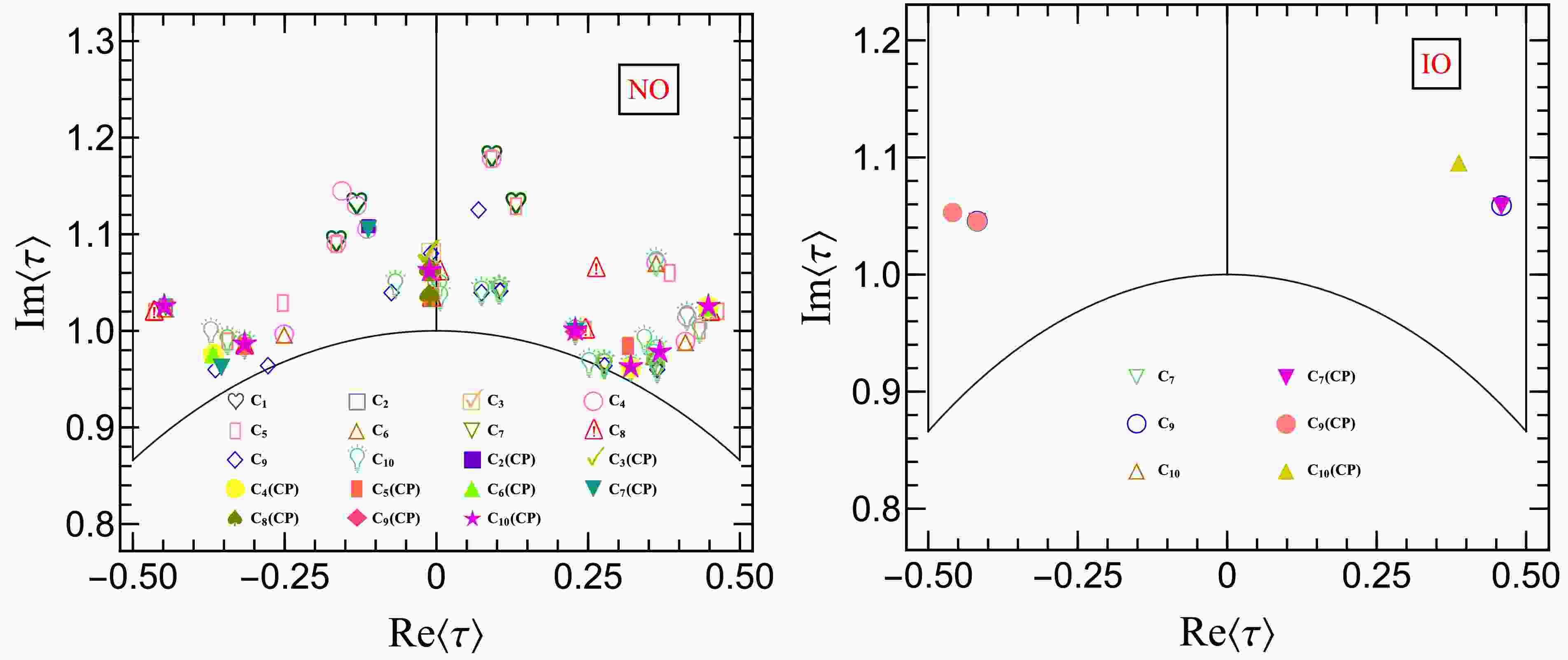
In all these models, the modulus τ is regarded as a free parameter to maximize the agreement between theoretical predictions and experimental data. The best fit values of the complex modulus τ in the fundamental domain of $ \mathrm{SL}(2,{\mathbb{Z}}) $ are displayed in figure 1. This analysis includes 194 viable models for the NO case (147 without CP and 47 with CP) and 11 for the IO case (6 without CP and 5 with CP). We find that the VEVs of τ in most viable models cluster near the regions $ \Re\tau = 0 $, $ |\tau| = 1 $ or $ \Re \tau = \pm0.5 $ for both mass orderings. The key observables for each model, which include the three lepton mixing angles, three CP-violating phases, $ \sum\nolimits_{i = 1}^{3} m_{i} $, $ m_{\beta\beta} $ and $ m_\beta $ are relevant to their minimal $ \chi^2 $ values. The corresponding results for the NO and IO cases are displayed in figures 2 and 4, and figures 3 and 5, respectively. Only a few models feature best fit values for all three mixing angles and the Dirac CP phase within the experimental $ 1\sigma $ ranges, indicating strong agreement with data, as shown in figures 2 and 3. The next-generation neutrino oscillation experiments and cosmological surveys will provide precise measurements of the lepton mixing parameters and neutrino masses. Combined with accurate determinations of $ m_{\beta\beta} $, the joint analysis of these experimental data will offer crucial evidence for investigating various modular models. Assuming the current best fit value for $ \sin^{2}\theta_{12} $ remains unchanged, the next-generation JUNO experiment will measure this parameter with high precision after six years of data collection. As shown in figures 2 and 3, its projected $ 3\sigma $ uncertainty range is wide enough to encompass the predicted $ \sin^{2}\theta_{12} $ values of almost all models considered. Distinguishing among these modular models will require improved precision on $ \theta_{23} $ and $ \delta_{CP} $. Future long baseline experiments DUNE [64] and T2HK [70] will critically test viable modular models through precision measurements of $ \theta_{23} $ and $ \delta_{CP} $. The projected angular resolution of these parameters in DUNE after 15 years running is also shown in the two figures. As these projections indicate, once DUNE and T2HK achieve their target sensitivity, the majority of the currently viable models will be decisively tested. The combination of JUNO, DUNE and T2HK will provide a powerful approach to testing these models. Given the projected constraints from these experiments, only a small number of models remain consistent with data, while the vast majority will be disfavored.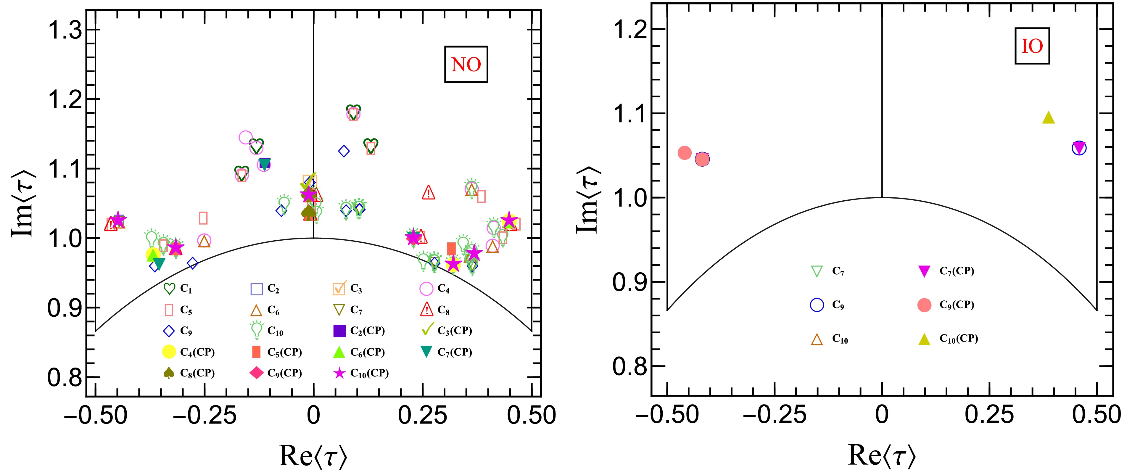

Figure 1.  The best fit values of modulus τ for 147 (47) and 6 (5) viable models in the case without (with) gCP symmetry for NO and IO neutrino mass spectra, respectively.

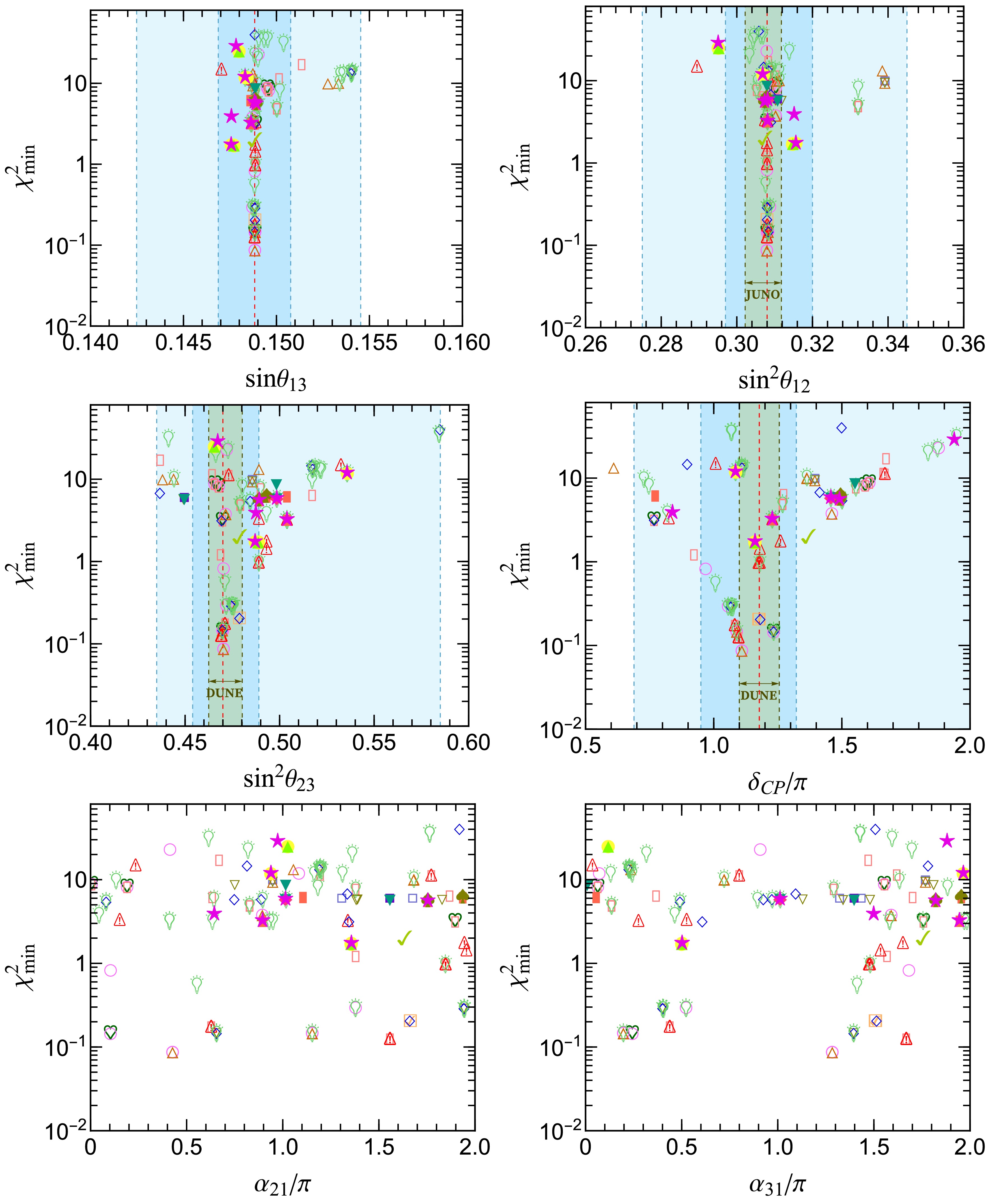
Figure 2.  The results of the best fit values of the minimum value of $\chi^2$, the three lepton mixing angles and three CP-violating phases for viable models without (147 models) and with (47 models) gCP symmetry in the NO case. The red dashed lines in the first four panels represent the best fit values, and the light blue bounds represent the $1\sigma$ and $3\sigma$ ranges from NuFIT 6.0 with Super-Kamiokande atmospheric data [62]. The lighter green band in the panel of $\sin^{2}\theta_{12}$ is the prospective $3\sigma$ range after 6 years of JUNO running [63]. The lighter green regions in the panels of $\sin^{2}\theta_{23}$ and $\delta_{CP}$ are the resolution in degrees after 15 years of DUNE running [64] for true values of them corresponding to their best fit values given by NuFIT 6.0.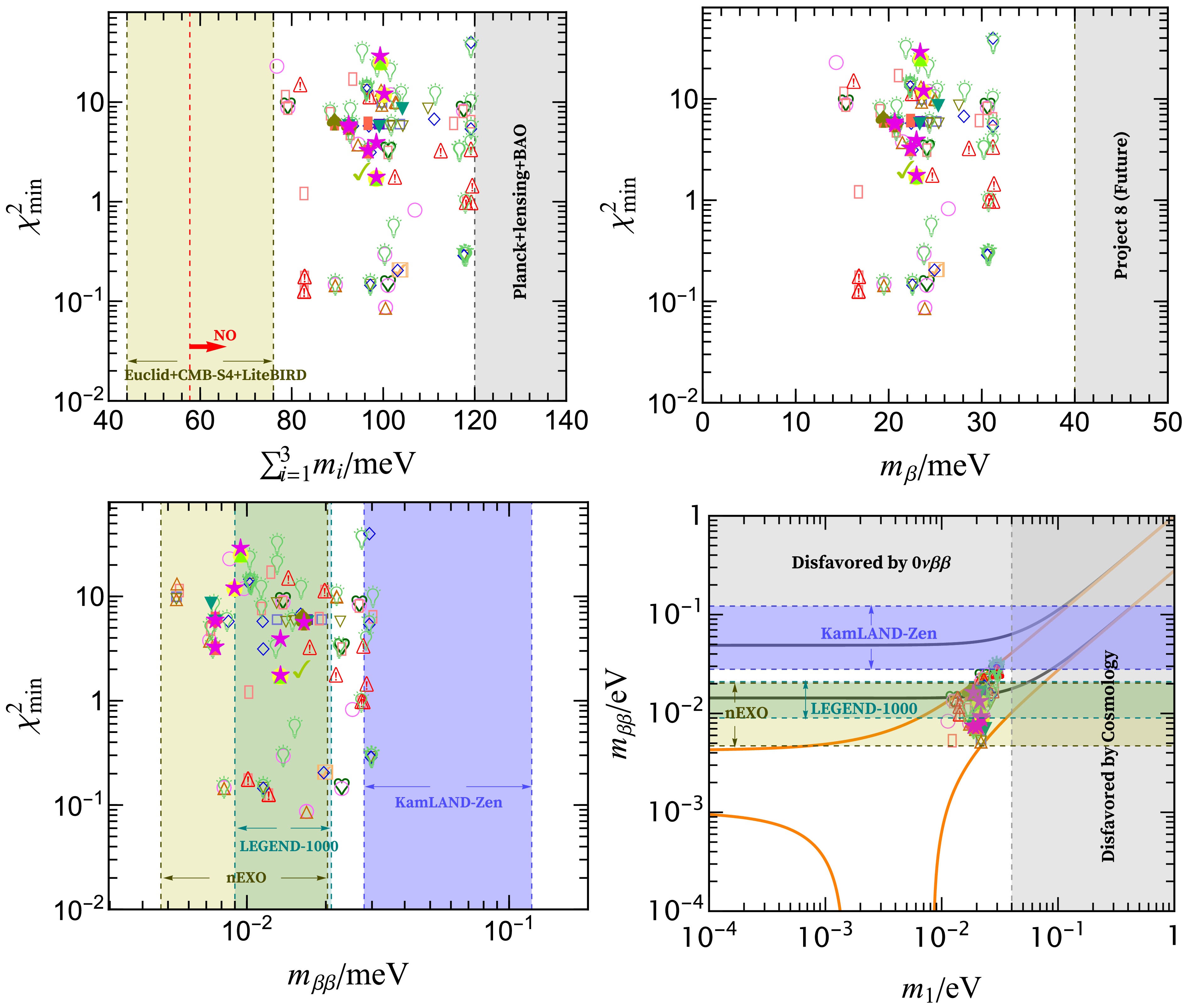

Figure 4.  The best fit values of the minimum value of $\chi^2$, the effective mass $m_{\beta\beta}$ in $0\nu\beta\beta$-decay, the kinematical mass $m_{\beta}$ in beta decay and the three neutrino mass sum $\sum_{i=1}^{3} m_{i}$. In the panel of the neutrino mass sum $\sum_{i=1}^{3} m_{i}$, the vertical bands indicate the current most stringent limit $\sum_{i=1}^{3} m_{i}<120\,\text{meV}$ from the Planck $+$ lensing $+$ BAO [61], the next-generation experiments sensitivity ranges $\sum_{i=1}^{3} m_{i}<(44-76)\,\text{meV}$ of Euclid+CMB-S4+LiteBIRD [65], and the red dashed line represents the limitation of the NO case ($\sum_{i=1}^{3} m_{i}\geq 57.75\,\text{meV}$). In the panel of the kinematical mass $m_{\beta}$ in beta decay, the gray region represents Project 8 future bound ($m_{\beta}<0.04\,\text{meV}$) [66]. In the panel of the effective Majorana mass $m_{\beta\beta}$, the vertical bands indicate the latest result $m_{\beta\beta}<(28-122)\,\text{meV}$ of KamLAND-Zen [67], and the next-generation experiments sensitivity ranges $m_{\beta\beta}<(9-21)\,\text{meV}$ from LEGEND-1000 [68] and $m_{\beta\beta}<(4.7-20.3)\,\text{meV}$ from nEXO [69].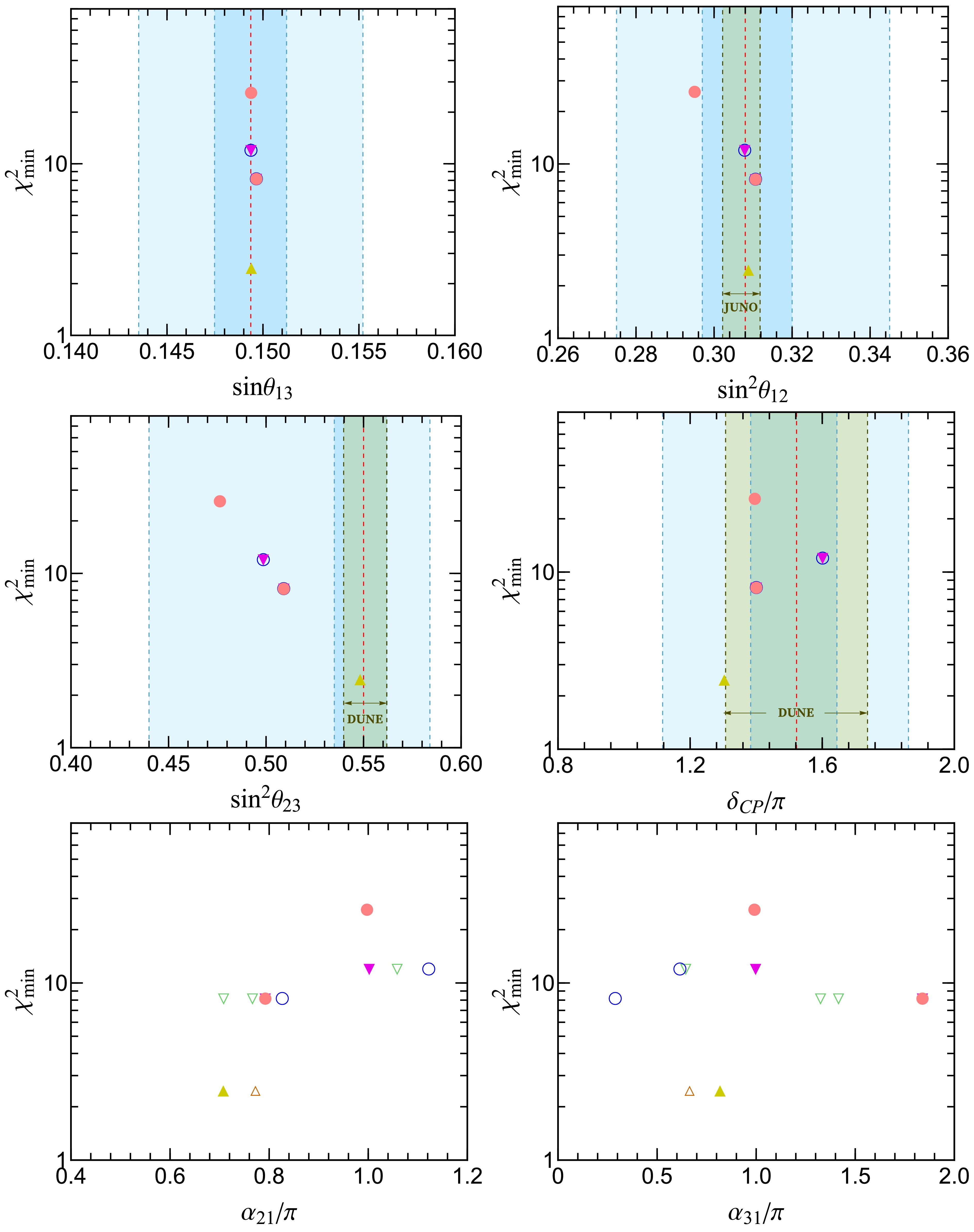

Figure 3.  The results of the best fit values of the minimum value of $\chi^2$, the three lepton mixing angles and three CP-violating phases for all viable models without and with gCP symmetry in the IO case.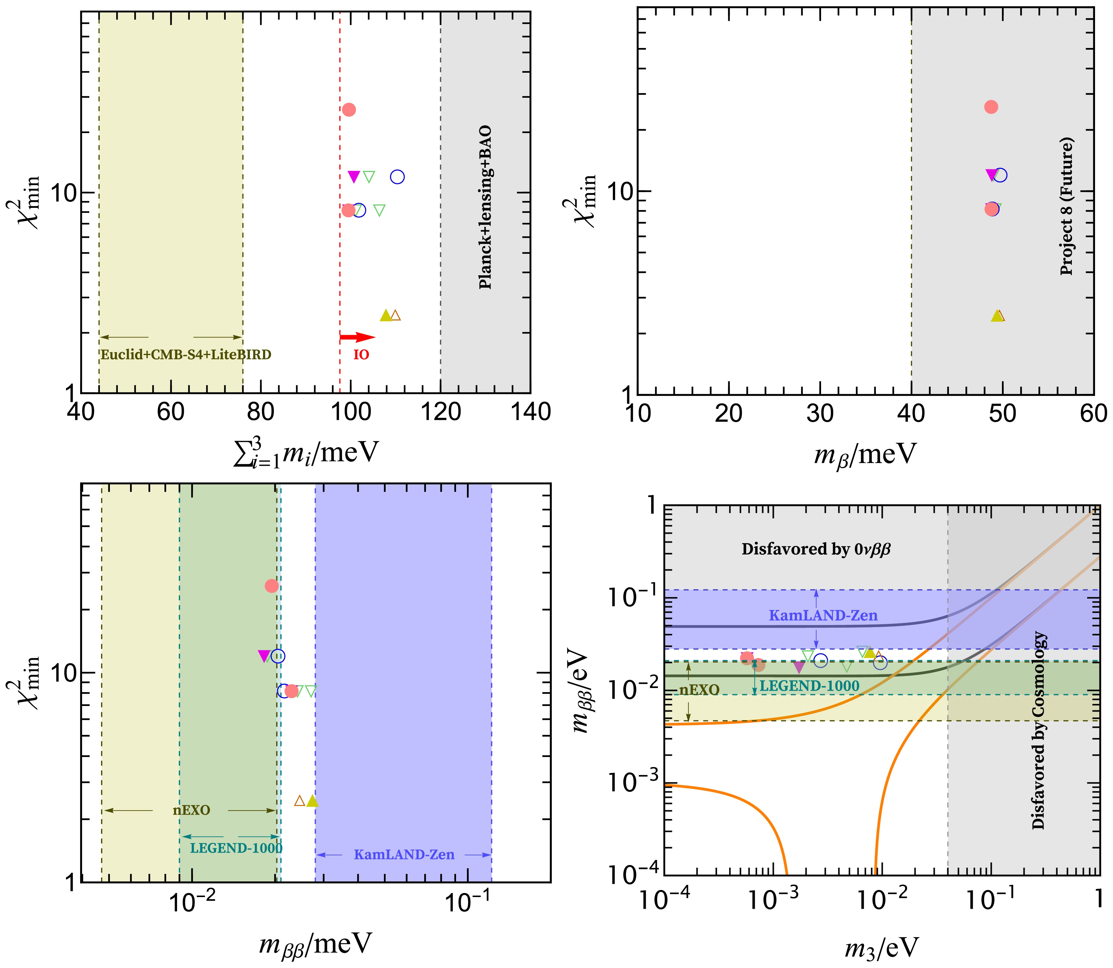

Figure 5.  The best fit values of the minimum value of $\chi^2$, the effective mass $m_{\beta\beta}$, the kinematical mass $m_{\beta}$ and the mass sum $\sum_{i=1}^{3} m_{i}$.

Figures 4 and 5 indicate that the predicted sum of neutrino masses $ \sum\nolimits_{i = 1}^{3} m_{i} $ for all viable models lies within the detection range of future cosmological surveys. These estimates lie within the projected $ 1\sigma $ sensitivity $ \sum\nolimits_{i = 1}^{3}m_i \lt (44-76)\, \text{meV} $ of the combined Euclid+CMB-S4+LiteBIRD analysis [65], which assumes a fiducial $ \sum\nolimits_{i = 1}^{3} m_i = 60\, \text{meV} $ with a $ 1\sigma $ uncertainty of $ 16\, \text{meV} $. Note that the minimal $ \sum\nolimits_{i = 1}^{3} m_i $ from oscillation data is approximately $ 59\, \text{meV} $ (NO) and $ 99\, \text{meV} $ (IO). The forecast $ \sum\nolimits_{i = 1}^{3} m_i \lt (44-76)\, \text{meV} $ is a sensitivity reach: achieving it would exclude IO and, for NO, indicate masses close to the minimal values. In figures 4 and 5, the lower bounds on the lightest neutrino mass $ m_{\text{lightest}} $ are derived from the cosmological limit $ \sum\nolimits_{i = 1}^{3} m_i \lt 120\,\text{meV} $ [61] combined with the measured mass squared differences. For NO, with $ m_{\mathrm{lightest}} = m_1 $,

using $ \Delta m_{21}^2 = 7.49\times10^{-5}\ \text{eV}^2 $ and $ \Delta m_{31}^2 = 2.513 \times 10^{-3}\ \text{eV}^2 $ gives $ m_1<39.989\ \text{meV} $. For IO, with $ m_{\mathrm{lightest}} = m_3 $,

using $ \Delta m_{32}^2 = -2.484\times10^{-3}\ \text{eV}^2 $ gives $ m_3<39.980\ \text{meV} $. For the NO case, all viable models yield $ m_{\beta} $ values below the forecasted detection limit of $ 0.04\ \text{eV} $ by Project 8 [66], while for the IO case, $ m_{\beta} $ lies above this threshold. Predictions for $ m_{\beta\beta} $ in all viable NO models are compatible with the current KamLAND-Zen constraint of $ m_{\beta\beta} \lt (28 - 122)\ \text{meV} $ [67], though this bound is expected to accommodate some viable IO models. Upcoming experiments such as LEGEND-1000 (aiming for $ m_{\beta\beta} \lt (9 \sim 21)\ \text{meV} $) [68] and nEXO (with a projected reach of $ m_{\beta\beta} \lt (4.7 \sim 20.3)\ \text{meV} $) [69] will be sensitive enough to test most of the NO models and all of the IO models. The relationship between the lightest neutrino mass ($ m_1 $ or $ m_3 $) and $ m_{\beta\beta} $ for each viable case is illustrated in figures 4 and 5, highlighting parameter trends across mass orderings.

Based on the above discussion, we identify 147 (47) minimal phenomenologically viable lepton flavor models for NO case and 6 (5) for IO case, and they are constructed using level 3 polyharmonic polyharmonic Maaß with even weights, associated with the finite modular group $ \Gamma_3\cong A_4 $ without (with) gCP symmetry. All of these models are characterised by six real parameters $ \alpha v $, $ \beta/\alpha $, $ \gamma/\alpha $, $ g_{1}v^{2}/\Lambda $, $ |g_{2}/g_{1}| $ and $ \Im \tau $, along with two phases $ {{\rm{Arg}}}(g_{2}/g_{1}) $ and $ \Re \tau $, when gCP symmetry is not imposed. If gCP symmetry is present, $ \Re \tau $ serves as the only phase parameter. The three real values $ \alpha v $, $ \beta/\alpha $ and $ \gamma/\alpha $ are determined by fitting the three charged lepton masses. The remaining three real parameters and two (or one) phases then determine the neutrino sector observables: the three neutrino masses, the three mixing angles, the Dirac CP-violating phase and two Majorana CP-violating phases entering the PMNS matrix. Since 9 neutrino observables are constrained by only 5 (or 4) independent parameters, these non-holomorphic $ A_{4} $ modular models are highly predictive. Consequently, non-trivial correlations among observables inevitably emerge, which can be derived through an analysis analogous to those presented in Refs. [18, 59]. A comprehensive analysis and a complete graphical examination of all viable models lie beyond the scope of this study. To demonstrate the predictive efficacy of non-holomorphic $ A_{4} $ modular invariant models, we focus on a representative model that effectively illustrates the quality of the obtained results. Next we present detailed numerical results for model $ \{C^{(2,4,2)}_{10},W_{3}\} $ as an illustrative example. The representation and weight assignments for the lepton fields in this model are as follows:

The resulting charged lepton and light neutrino mass matrices can be obtained from table 2 and Eq. (6) respectively:

where the explicit matrix elements are determined by polyharmonic Maaß forms of respective weights. This model can produce results consistent with experimental data for both NO and IO mass spectra, under conditions both with and without gCP symmetry. The predicted best fit values of input parameters and physical observable quantities are summarized in tables 4, 5, 6 and 7.

After performing exhaustive scans of the model's parameter spaces while requiring all observables to remain within their experimental 3σ ranges from NuFIT [58], we find that the three lepton mixing angles and the three CP violation phases are constrained within narrow ranges for both mass hierarchies:

for model $ \{C^{(2,4,2)}_{10},W_{3}\} $ without (with) gCP symmetry. It is remarkable that the atmospheric mixing angle $ \theta_{23} $ is very closed to its maximal value for NO case. When gCP symmetry compatible with the $ A_4 $ modular symmetry is imposed, all CP-violating phases are confined to narrow intervals. The reason is that gCP invariance requires all couplings to be real, so CP violation can only arise from $ \Re\tau $. Additionally, the Majorana CP phases $ \alpha_{21} $ and $ \alpha_{31} $ deviate slightly from their trivial values. These precise constraints imply that the model can be tested experimentally at upcoming long baseline neutrino facilities DUNE and T2HK which are highly sensitive to Dirac CP-violating phase and atmospheric mixing angle. The neutrino mass parameters $ \sum\nolimits_{i = 1}^{3} m_{i} $ and $ m_{\beta\beta} $ are constrained across both mass orderings. For the NO case, $ \sum\nolimits_{i = 1}^{3} m_{i} $ falls in the sensitivity reach of upcoming cosmological surveys such as Euclid+CMB-S4+LiteBIRD, while $ m_{\beta\beta} $ lies below the current KamLAND-Zen limit but could be accessible to next-generation experiments like LEGEND-1000 and nEXO. In contrast, for the IO case, both parameters lie within projected detection ranges of future experiments, offering a clear avenue to distinguish between mass orderings.

Furthermore, we identify several notable correlations between input parameters and physical observables. Specifically, clear dependencies are found between $ \Re\tau $ and $ \Im\tau $, as well as between the Dirac CP phase $ \delta_{CP} $ and $ \Re\tau $. These correlations are separately illustrated for the NO and IO mass spectra in figures 6 and 7, respectively, where green (red) points denote results obtained without (with) the imposition of gCP symmetry. Among the mixing observables, correlations are established between $ \sin^2\theta_{23} $ and $ \sin^2\theta_{13} $, $ \sin^2\theta_{12} $, $ \delta_{CP} $ and the Majorana phase $ \alpha_{21} $ (see figures 6 and 7 for NO and IO cases respectively). Notably, $ \theta_{23} $ is strongly correlated with the other mixing parameters, in particular with the parameters fixed by gCP symmetry. Moreover, a strong correlation exists between the Dirac CP phase $ \delta_{CP} $ and the solar mixing angle $ \theta_{12} $. Such predicted interplays can be tested in the future by combining precision measurements from the JUNO experiment with data from long baseline oscillation facilities such as DUNE or T2HK. In contrast, for our chosen model, the total neutrino mass sum $ \sum\nolimits_{i = 1}^{3}m_{i} $ and the effective mass $ m_{\beta\beta} $ do not show correlations with the mixing parameters as strong as those reported in Ref. [59], especially when CP symmetry is not enforced.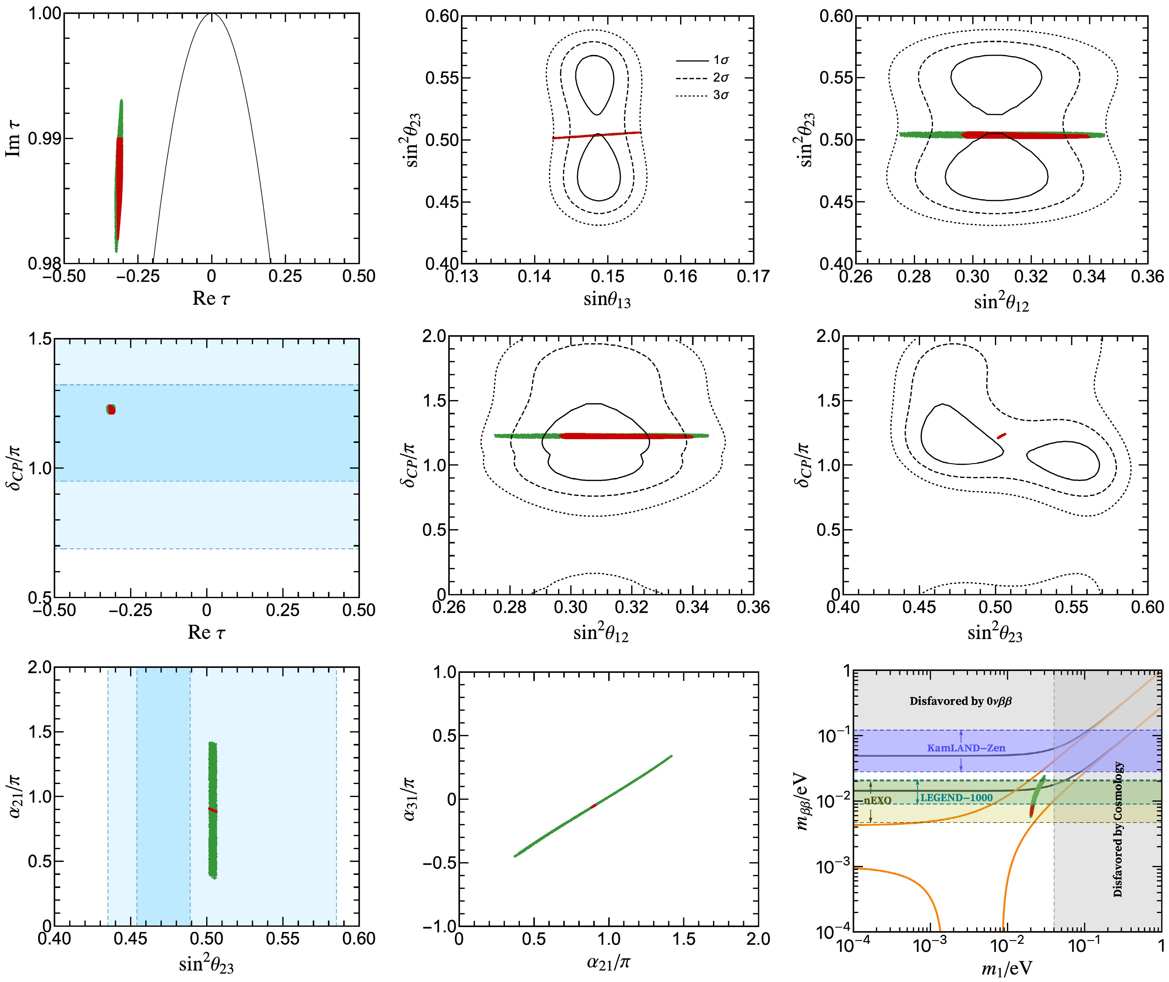

Figure 6.  The predicted correlations among the input parameters, lepton mixing angles and CP-violating phases in the model $\{C^{(2,4,2)}_{10},W_{3}\}$ with (red) and without (green) gCP symmetry for NO neutrino mass spectrum.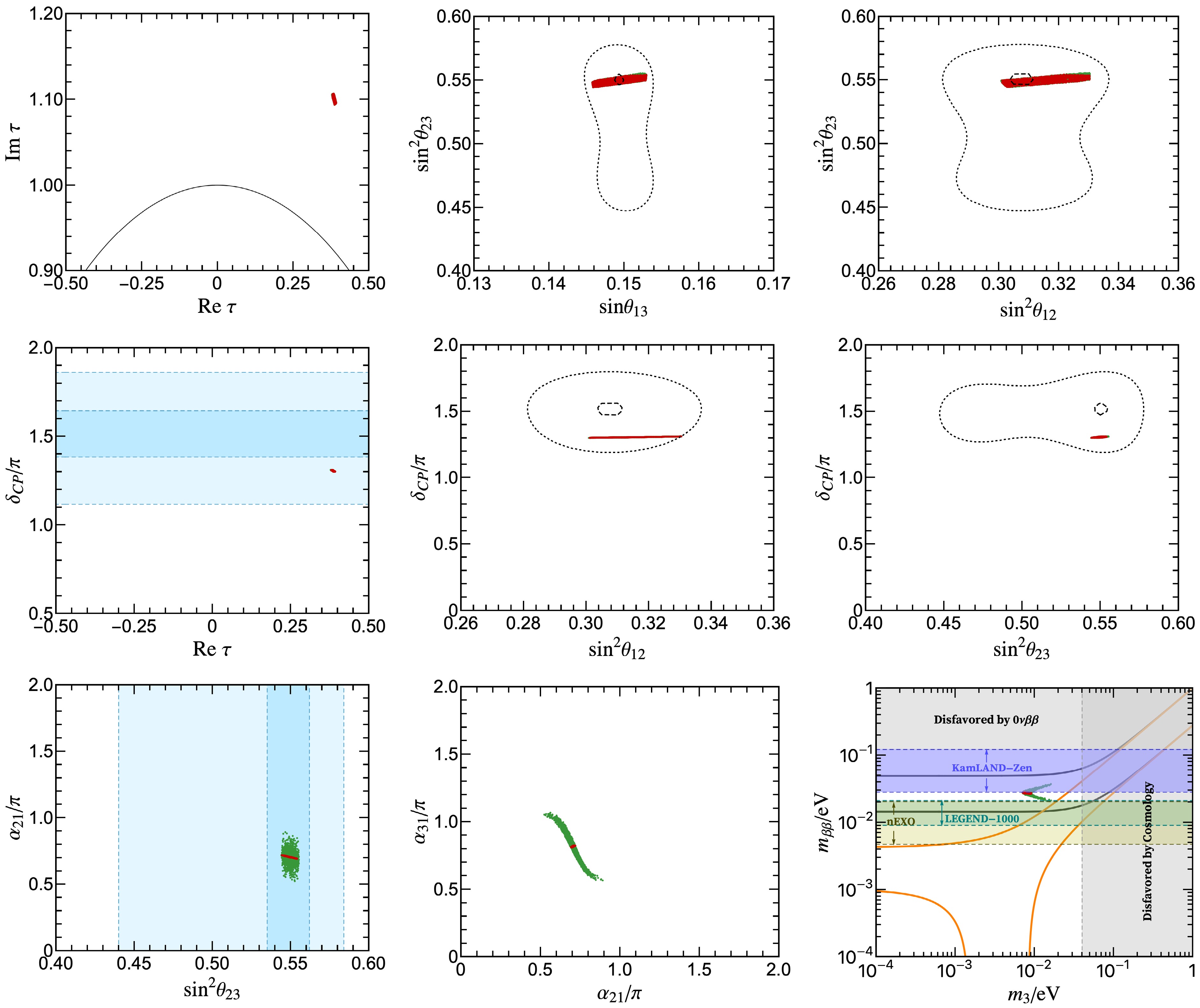

Figure 7.  The predicted correlations among the input parameters, lepton mixing angles and CP-violating phases in the model $\{C^{(2,4,2)}_{10},W_{3}\}$ with (red) and without (green) gCP symmetry for IO neutrino mass spectrum.

The modular invariance is a promising framework to describe the masses and mixing parameters of both quarks and leptons [13]. In the framework of original modular symmetry, SUSY is a necessary component. In this context, the principle of modular invariance forces the Yukawa couplings to be level N modular forms which are holomorphic functions of the complex modulus τ. However, there is no evidence for low-energy supersymmetry. Subsequently, a non-supersymmetric formulation of the modular flavor symmetry was recently proposed in Refs. [33, 50]. This approach extends the standard level N modular forms by polyharmonic Maaß forms, a class of non-holomorphic modular forms that exist for zero, negative and positive integer weights. The framework of non-holomorphic modular flavor symmetry presents a novel avenue for understanding the flavor structure of fermions.

In the present work, we perform a systematic analysis of all minimal lepton models based on non-holomorphic $ \Gamma_3 \cong A_4 $ modular symmetry. These models are explicitly constructed using only the modulus τ, with no additional flavons. In these models, light neutrino masses are generated by the effective Weinberg operator, while the Yukawa couplings are derived from polyharmonic Maaß forms of level 3 with even weights k in the range $ -4 \leq k \leq 4 $. The three LH lepton doublets transform as the $ A_4 $ triplet 3, while the RH charged leptons $ E^c_{1,2,3} $ are assigned to $ A_4 $ singlets 1, $ {{\bf{1}}^{\bf{\prime}}} $ or $ {{\bf{1}}^{{\bf{\prime\prime}} }}$. According to the representation and weight assignments for the lepton fields, we identified 1820 independent minimal models, each depending on eight real parameters: the six dimensionless inputs in Eq. (9) and two overall scales. When the non-holomorphic $ A_{4} $ modular flavor symmetry is extended to combine with gCP symmetry, then one more free parameter would be reduced for all these models. By numerically minimizing the $ \chi^{2} $ function for each model, we find out 147 (6) phenomenologically viable models for the NO (IO) mass spectrum. Among these, only 47 (5) remain consistent with experimental data from the lepton sector when gCP is imposed. The corresponding best fit values of input parameters, lepton masses, lepton mixing angles, CP-violating phases, the 0$ \nu\beta\beta $-decay effective Majorana mass and the kinematical mass are comprehensively presented in tables 4, 5, 6 and 7. Based on our predictions, the current JUNO constraint on $ \sin^{2}\theta_{12} $ rules out only 5 of the 147 viable NO models without gCP symmetry, while all others remain consistent with experimental data. The future experimental results can significantly constrain the set of currently viable models. If the current best-fit value of $ \sin^{2}\theta_{12} $ remains unchanged, JUNO will determine this parameter with high precision after six years of data. However, its projected $ 3\sigma $ interval still covers the $ \sin^{2}\theta_{12} $ predictions of almost all models considered. The next-generation long baseline experiments like DUNE and T2HK are projected to determine the atmospheric mixing angle $ \theta_{23} $ with unprecedented precision, which will rule out a large fraction of models. Additional constraints are expected from refined measurements of the Dirac CP-violating phase $ \delta_{CP} $, the sum of neutrino masses $ \sum\nolimits_{i = 1}^{3}m_{i} $ and the effective Majorana mass $ m_{\beta\beta} $ of 0$ \nu\beta\beta $-decay.

To illustrate our findings more clearly, we present detailed numerical results for the example model $ \{C^{(2,4,2)}_{10}, W_{3}\} $, demonstrating how the non-holomorphic $ A_{4} $ modular flavor symmetry can be applied to address the flavor problem. We present complete predictions for lepton mixing parameters, neutrino masses, and the effective mass of $ 0\nu\beta\beta $-decay under both NO and IO spectra, with and without gCP symmetry. Our analysis reveals several non-trivial correlations between input parameters and physical observables for both mass orderings. Furthermore, imposing gCP symmetry markedly reduces the allowed parameter space and yields much sharper, more definitive correlations. All these theoretical predictions can be rigorously tested by next-generation neutrino experiments. Most notably, the specific predictions of this model will face decisive verification from next-generation $ 0\nu\beta\beta $-decay experiments such as LEGEND-1000 and nEXO.