Resonant states in the Schrödinger equation solved by the Green's function method

Resonant states are commonly observed in atomic, nuclear and particle physics. Among all kinds of resonances, one-particle shape resonance is the simplest case that arises in potential scattering of a particle by an unexcited target or simply in a potential field with a confining potential barrier [1]. In nuclear physics, since Tanihata et al. discovered the neutron halo in $ ^{11}\mathrm{Li} $ in 1985 [2], people found that the continuum spectrum, especially the low-lying resonant states with a small angular momentum l therein, plays an important role in nuclei far from the β-stability line [3−5]. In addition, the single-particle resonances also provide the main contribution to many collective excitations such as giant resonances [6, 7].

There have been many theoretical methods developed to study the single-particle resonant states in a given potential. Some of these methods are based on traditional scattering techniques, such as the R-matrix method [8, 9], scattering matrix (SM) method [7, 10−13], K-matrix method [14], Jost function method [15−17], and scattering phase shift method [18−20]. On the other hand, some methods originally used for studying bound states have been extended to study the single-particle resonant states, including the complex scalar method (CSM) [21−25], analytical continuation of the coupling constant (ACCC) method [26−30], real stability method (RSM) [31, 32], complex momentum representation (CMR) method [33−37], and the complex scalar Green's function method (CGF) [38−40].

The Green's function (GF) [41−46], as a useful mathematical tool, can provide another choice for solving the single-particle resonant states. Actually, it can simultaneously provide the information for both bound and continuum states, depending on the boundary conditions. In the non-relativistic mean-field model, the GF was firstly used in the Hartree-Fock-Bogoliubov (HFB) theory to treat the continuum quasiparticle states in the presence of pairing [42, 47]. Then the GF was used to calculate densities needed in the self-consistent density functionals [48−50], where the quasiparticle resonances can be identified from the occupation number density and pair number density [48, 51]. In the relativistic counterpart, the relativistic mean-field theory formulated with Green's function was first introduced in 2014 and successfully applied to study the single-neutron resonant states [52]. The study was extended for the single-proton and single-hyperon resonant states, respectively [53, 54]. Combined with the relativistic continuum Hartree-Bogoliubov (RCHB) theory, the RCHB with Green’s function method was also constructed to investigate the quasiparticle resonances and halo phenomena near the drip line [55, 56]. Note in above studies, the resonance energy and width were read from the peak of density of states (DOS) calculated by GF subtracting the contribution from the free scattering states (denoted by GFI). Subsequently, two additional recipes were proposed in order to determine the resonant energies and widths of broad resonances with higher precision. Refs. [57, 58] proposed to scan the DOS in the fourth quadrant of complex energy plane and identify the resonance states as the flip of DOS when crossing the poles of GF (denoted by GFII), while Refs. [59, 60] proposed to search the resonant states directly as the poles of GF in the fourth quadrant of complex energy plane (denoted as GFIII).

The above three recipes GFI, GFII and GFIII have been developed to find the resonant states in the Dirac equation. In this paper, we will check the feasibility of these recipes to identify the single-neutron resonances in the Schrödinger equation. By taking the Woods-Saxon type mean-field and spin-orbit potentials in $ ^{40} \mathrm{Ca} $ as an example, the DOS will be calculated out with the GF method for both bound and continuum states. Then the single-neutron resonant energies and widths will be determined by GFI, GFII, and GFIII methods respectively, and we will compare their results in detail. The paper is organized as follows: Section 2 presents the theoretical framework to solve the Schrödinger equation with GF method; Section 3 discusses the DOSs for the bound and resonant states obtained by the GF method, and compares in detail the energies and widths of the resonant states obtained by the three recipes; Finally, a summary is presented in Section 4.

The stationary Schrödinger equation is:

where H is the single-particle Hamiltonian, ϕ is the single-particle wave function, and $ \epsilon $ is the corresponding energy. The Hamiltonian can be written as

with μ representing the mass of the neutron and $V({\boldsymbol{r}})$ the single-particle potential. Here $V({\boldsymbol{r}})$ includes the Woods-Saxon mean-field potential $ V_q(r) $ and the spin-orbit potential $ V_{ls}(r) $ with the spherical symmetry

in which

and

The single-particle GF for the Schrödinger equation (1) is defined as:

with $ {\boldsymbol{r}} $ representing the space coordinate and σ the spin of the particle. This GF can be expressed by a complete set of eigenstates $ \phi_n({\boldsymbol{r}} \sigma) $ and the corresponding eigenvalues $ \epsilon_n $ of the Hamiltonian H, i.e.,

Obviously, the eigenstates of the Schrödinger equation are the poles of the GF. In the DOS [61]

the bound states will show up as δ peaks at real $ \epsilon_n $. The resonant states locate in the fourth quadrant of the complex energy plane with the energies $ \epsilon_n=\varepsilon_R-\mathrm{i} \Gamma / 2 $, where $ \varepsilon_R $ and Γ are the resonance energy and width, respectively [57, 62]. It can be demonstrated that, the DOSs can be calculated by the integrals of the GF in the coordinate $ {\boldsymbol{r}} $ space as

In a spherical system, the DOSs can be written as a superposition of the partial wave DOSs,

with l and j as the angular momenta of the partial wave. On the other hand, the GF can also be expanded as

where $ \mathrm{Y}_{ljm}(\theta, \phi) $ is the spin spherical harmonic, and $ \mathcal{G}_{lj} $ represents the radial Green's function with the angular momenta l and j. Therefore, for a partial wave state with fixed quantum numbers l and j, the DOS is given by:

The radial GF $ \mathcal{G}_{lj}\left(r, r^{\prime}, \epsilon\right) $ can be calculated as:

where $ \theta(r-r^{\prime}) $ is the step function and $ w(\epsilon) $ is the r-independent Wronskian function defined by

The wave functions $ u_{lj}^{(1)}(r) $ and $ u^{(2)}_{lj}(r) $ satisfy the radial Schrödinger equation,

and are obtained from the asymptotic behaviors at $ r \rightarrow 0 $ and $ r \rightarrow \infty $, respectively. At $ r \rightarrow 0 $, the radial wave function $ u^{(1)}_{lj}(r) $ is regular and can be expanded into powers of r as in the SM approach [13]. At $ r\rightarrow \infty $, the radial wave function $ u^{(2)}_{lj}(r) $ satisfies,

where $ k^2=\dfrac{2\mu\epsilon}{\hbar^2} $ and $ h_l^{(1)}(k r) $ is the spherical Hankel function of the first kind. One should notice that, for the bound states with the real negative energy $ \epsilon $, the spherical Hankel function of the first kind $ h_l^{(1)}(k r) $ with imaginary argument $ kr $ can be reduced to an exponential decaying function of the coordinate r in the asymptotic region. While, for the continuum states with a positive real part of energy, $ h_l^{(1)}(k r) $ can be reduced to an oscillating function of r in the asymptotic region. Therefore, the outside boundary condition in Eq. (16) naturally considers the different asymptotic behaviors for bound and continuum states according to their energies. As a result, both the bound and continuum states can be included in the GF (13) using the same form of boundary conditions.

In the following, we take the single-neutron potential of $ {}^{40} $Ca as an example to examine the bound and resonant states in the Schrödinger equation obtained by the GF method. The corresponding parameters of the Woods-Saxon potential (3) are taken as $ V_0=-57.0\ \mathrm{MeV} $, $ a=0.67\ \mathrm{fm} $, $ R=4.06945\ \mathrm{fm} $, and $ \frac{\hbar^2}{2\mu}=20.22671\ \mathrm{MeV}\cdot\mathrm{fm^2} $. In order to identify the resonant states, we follow three different methods using the GF as mentioned in Sec. I. To check the stability of the results of the resonant states, the coordinate space is chosen as $ R_{\text {box }} = 10, 20, 30\ \mathrm{fm} $ and with a mesh size of $ \mathrm{d} r = 0.1\ \mathrm{fm} $.

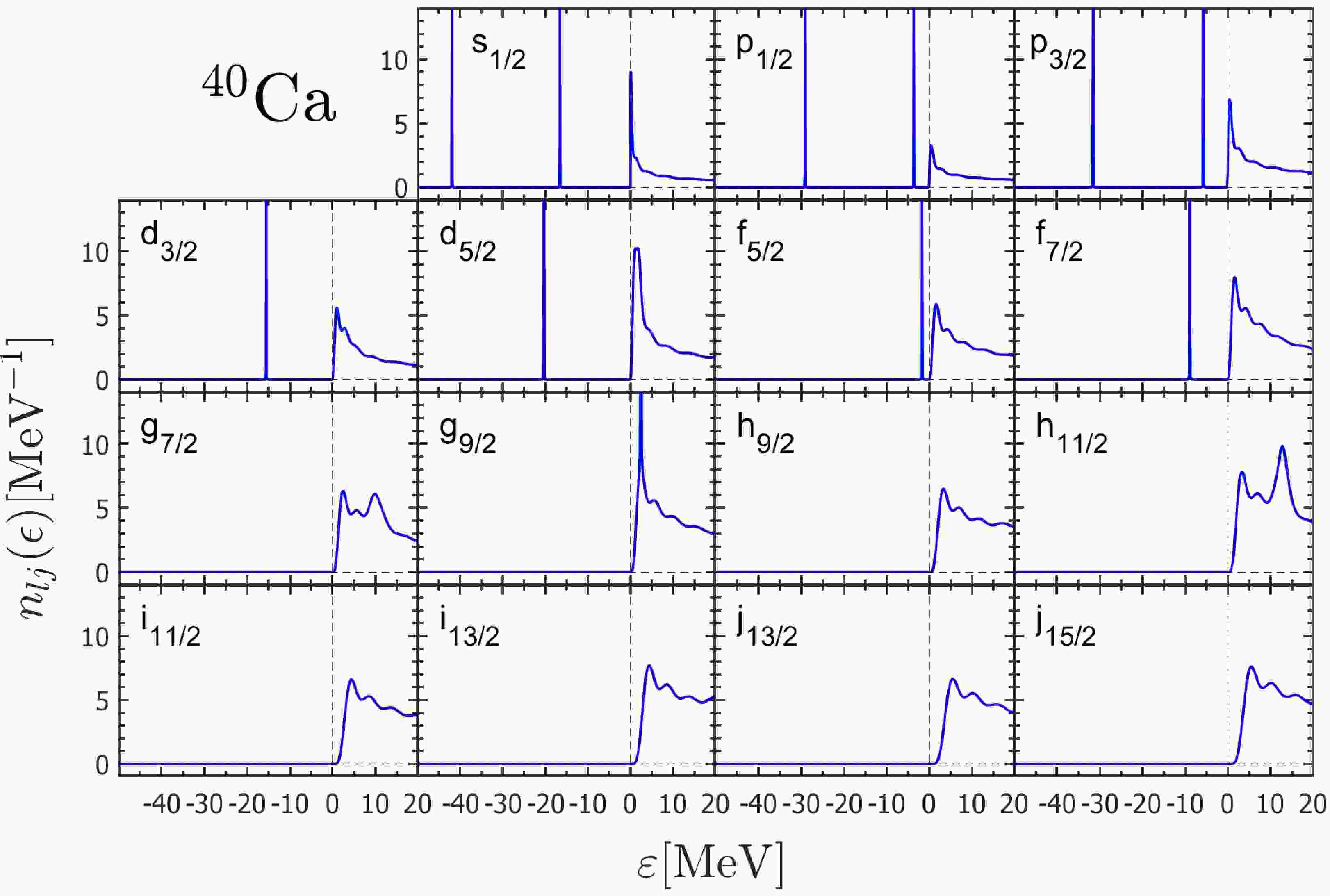
In the first method GFI [52], the partial wave DOS $ n_{lj}(\epsilon) $ (12) can be calculated by the integral of the GF in the coordinate space with a complex energy $ \epsilon=\varepsilon+\mathrm{i}\kappa $, where ε and κ are both real numbers representing the real and imaginary part of energy respectively. In this method, the imaginary part of energy κ has a fixed small positive value $ 1 \times 10^{-3}\ \mathrm{MeV} $ to visualize the δ peak for the bound state (if any). One can plot the DOS $ n_{lj}(\epsilon) $ as a function of the real part of energy ε to search the bound or resonant states. The energy step to plot $ n_{lj}(\epsilon) $ is taken as $ \mathrm{d} \varepsilon=1 \times 10^{-3}\ \mathrm{MeV} $. With both the given mean-field and spin-orbit potentials in Eq. (3), the calculated DOSs $ n_{lj}(\epsilon) $ are shown in Fig. 1 for different partial waves obtained with the box size $ R_{\rm box}=20 $ fm.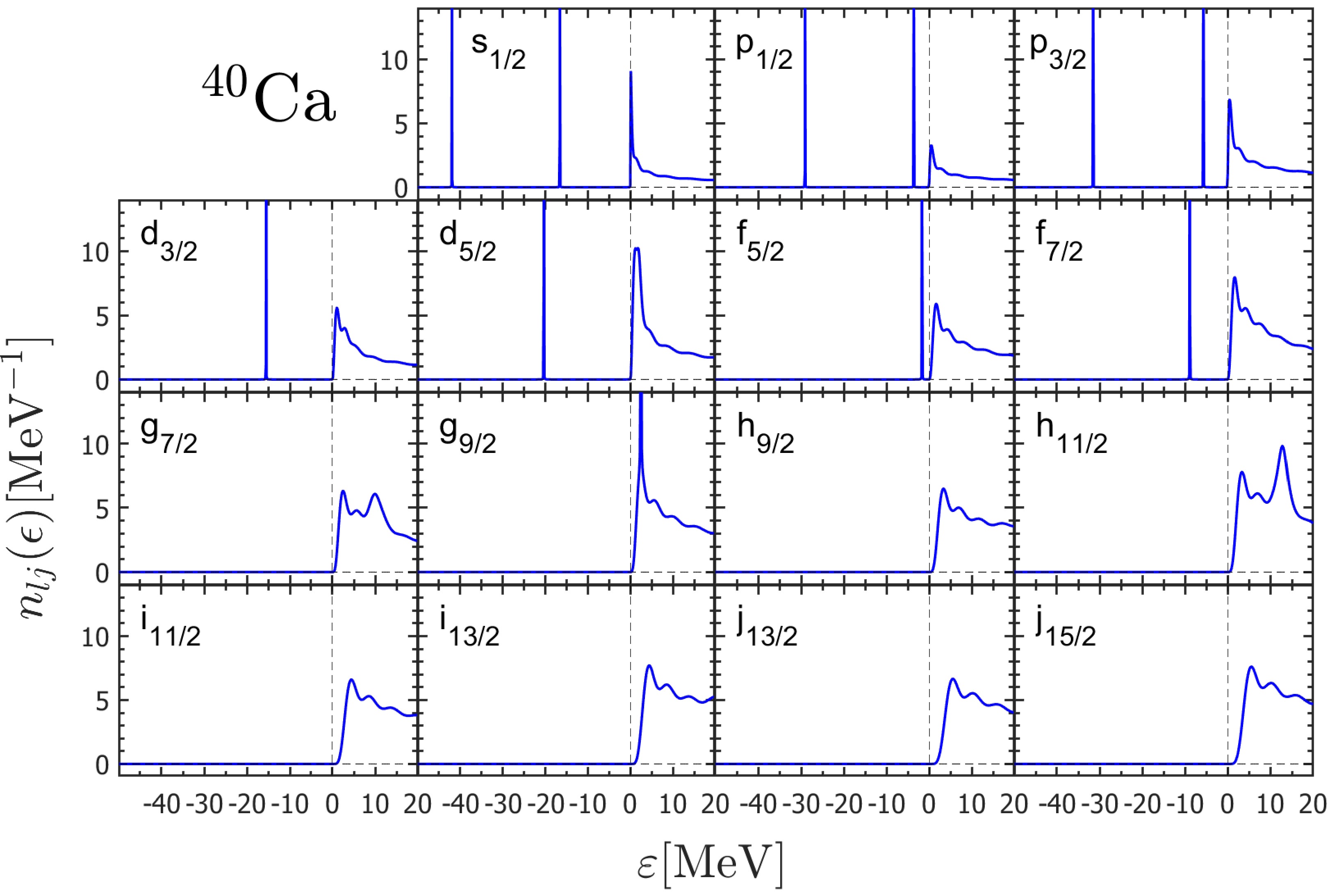

Figure 1.  (color online) The neutron DOSs $ n_{lj}(\epsilon) $ ($ \epsilon=\varepsilon+\mathrm{i}\kappa $ with $ \kappa=1 \times 10^{-3}\ \mathrm{MeV} $) for different partial waves in $ { }^{40} \mathrm{Ca} $ calculated by GF method with Woods-Saxon type mean-field and spin-orbit potentials in the box $ R_{\text {max }}=20\ \mathrm{fm} $ (solid line). The dashed vertical line at $\varepsilon = 0$ marks the continuum threshold.

In the energy region $ \varepsilon<0 $, the bound state (if any) will show up as a sharp peak with an artificial width $ 2\kappa $. As seen in Fig. 1, one can read the bound state energies at the peaks in $ s_{1/2}, p_{1/2}, p_{3/2}, d_{3/2}, d_{5/2}, f_{5/2} $, and $ f_{7/2} $ partial waves. These energies are listed in Table 1, in comparison with the results obtained by the shooting method with the box boundary condition in the same coordinate space. As shown, the single-neutron energies of bound states obtained from the two methods consist with each other within a precision of $ 10^{-3} $ MeV, which is determined by the energy step $ \mathrm{d} \varepsilon $.

$ nlj $	GFI	Shooting
$ 1{s}_{1/2} $	−41.961	−41.9607
$ 2{s}_{1/2} $	−16.587	−16.5870
$ 1{p}_{1/2} $	−29.077	−29.0770
$ 2{p}_{1/2} $	−3.557	−3.5572
$ 1{p}_{3/2} $	−31.508	−31.5080
$ 2{p}_{3/2} $	−5.648	−5.6479
$ 1{d}_{3/2} $	−15.466	−15.4658
$ 1{d}_{5/2} $	−20.349	−20.3493
$ 1{f}_{5/2} $	−1.630	−1.6298
$ 1{f}_{7/2} $	−8.838	−8.8379

Table 1.  The single-neutron energies (in MeV) of bound states in $ ^{40} $ Ca obtained by the GFI method and the shooting method. The box size $ R_{\text{box}} = 20 \, \mathrm{fm} $ and the mesh size $ \mathrm{d} r = 0.10\ \mathrm{fm} $ are adopted.

Just above the continuum threshold $ \varepsilon=0 $, the DOS shows sharp upward inclines with some peaks or oscillations above. According to Ref. [52], this is mainly contributed from the free particle scattering states. In order to remove their contributions, one could subtract the DOS $ n^0_{lj}(\epsilon) $ calculated with only centrifugal barrier but no mean-field potentials $ (V_q(r)=0) $ from the total DOS $ n_{lj}(\epsilon) $ and obtain the residual DOS $ n_{lj}^r(\epsilon)=n_{lj}(\epsilon)-n_{lj}^0(\epsilon) $ that is contributed only from the resonant states (if any). From the residual DOS, one can identify the resonant states and obtain the corresponding energy and width information.

The neutron DOSs $ n_{lj}(\epsilon), n^0_{lj}(\epsilon) $, and $ n^r_{lj}(\epsilon) $ above the continuum threshold for different partial waves in $ ^{40} $Ca calculated by GF are shown in Fig. 2. From the residual DOSs $ n^r_{lj}(\epsilon) $, one can see some obvious peaks in $ d_{5/2} $, $ g_{7/2} $, $ g_{9/2} $, $ h_{11/2} $ and $ i_{13/2} $ partial waves, which clearly correspond to the resonant states. One can take the peak energy as the resonant energy and the full width at half maximum (FWHM) to calculate the resonant width Γ,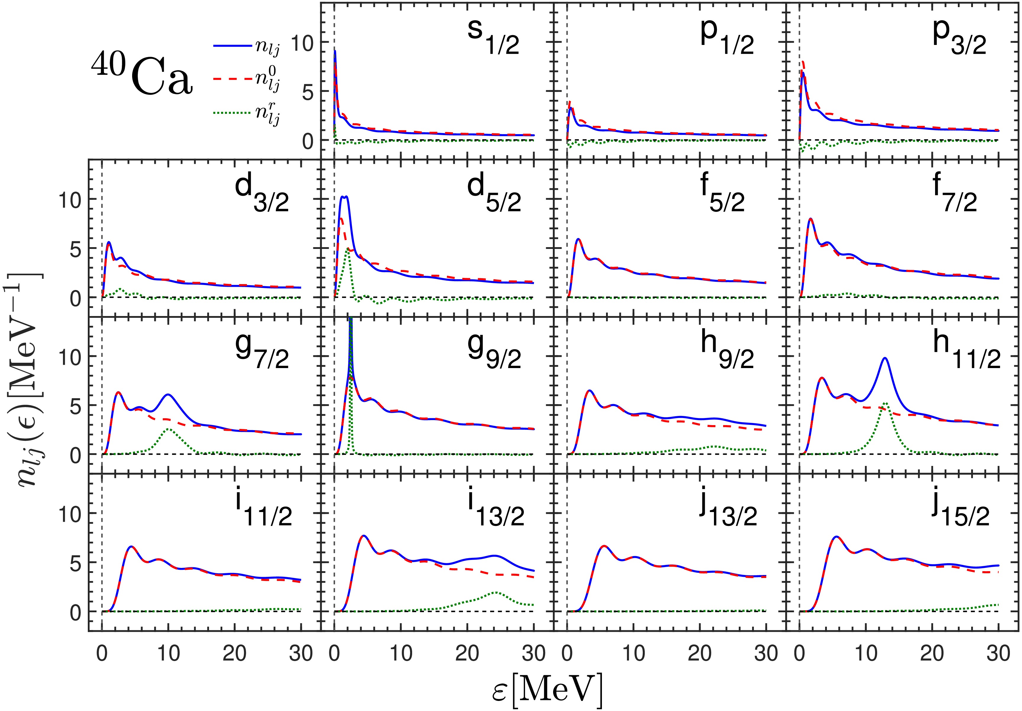

Figure 2.  (color online) Neutron DOSs $ n_{lj}(\epsilon) $ ($ \epsilon=\varepsilon+\mathrm{i}\kappa $ with $ \kappa=1 \times 10^{-3}\ \mathrm{MeV} $) for different angular momentum partial waves in $ { }^{40} \mathrm{Ca} $ calculated by GF method with Woods-Saxon type mean-field and its spin-orbit potentials (solid line), with only centrifugal barrier $ n^0_{lj}(\epsilon) $ (dashed line) and their differences $ n^r_{lj}(\epsilon)=n_{lj}(\epsilon)-n^0_{lj}(\epsilon) $ (dotted line) in the box $ R_{\rm box}=20 $ fm. The dashed vertical line at $\varepsilon = 0$ marks the continuum threshold.

Among these partial waves, $ g_{9/2} $ has a typical sharp resonant state at the energy $ \varepsilon_R=2.478 $ MeV with a quite small width $ \Gamma=0.023 $ MeV. Since the energy step is taken as $ \mathrm{d} \varepsilon=1 \times 10^{-3}\ \mathrm{MeV} $, the extracted energy and width are also truncated to the third decimal place ($ 10^{-3} $ MeV). In contrast, the residual DOS $ n^r_{lj}(\epsilon) $ in $ d_{3/2} $ partial wave has some small peaks within a wide energy region $ 2\sim 8 $ MeV. It is difficult to identify the energy and width of resonant state here. Taking $ g_{9/2} $ and $ d_{3/2} $ as two distinct examples, their DOSs $ n^r_{lj}(\epsilon) $ are zoomed in and compared in Fig. 3. To check the dependence of the DOSs on the box sizes, we also show the results calculated with box sizes $ R_{\rm box}=10 $ and $ 30 $ fm. For the narrow resonance in $ g_{9/2} $ partial wave in Fig. 3 (a), the peak structures calculated with different $ R_{\rm box} $ are almost the same. As a result, the resonant energy and width read from the peaks calculated with different box sizes are identical, as shown in Table 2 (GFI). In contrast, for the broad resonance in $ d_{3/2} $ partial wave in Fig. 3 (b), the DOS $ n^r_{lj}(\epsilon) $ changes significantly with different box size. One could still take the center energy of the highest peak as the resonant energy and the corresponding FWHM for the resonant width. The results thus obtained are also listed in Table 2 (GFI). It is obvious to see that the obtained energy and width for the broad $ d_{3/2} $ resonance sensitively depends on the adopted box size.

Figure 3.  (color online) The residual DOSs $ n_{lj}^r(\epsilon) $ ($ \epsilon=\varepsilon+\mathrm{i}\kappa $ with $ \kappa=1 \times 10^{-3}\ \mathrm{MeV} $) calculated with different box sizes $ R_{\rm box}=10, 20, 30 $ fm are shown for (a) $ g_{9/2} $ and (b) $ d_{3/2} $ partial waves. The same mesh size $ \mathrm{d}r=0.1 $ fm is adopted.

$ nl_j $		$ 10\ \mathrm{fm} $		$ 20\ \mathrm{fm} $		$ 30\ \mathrm{fm} $
		$ \varepsilon_R $	Γ	$ \varepsilon_R $	Γ	$ \varepsilon_R $	Γ
$ 2{d}_{3/2} $	GFI	2.902	2.356	2.732	1.674	2.556	3.196
	GFII	2.7143	4.8350	2.7133	4.8498	2.7133	4.8496
	GFIII	2.7143	4.8350	2.7133	4.8496	2.7133	4.8496
	SM	2.7140	4.8362	2.7133	4.8500	2.7133	4.8500
$ 2{d}_{5/2} $	GFI	1.860	1.096	1.946	1.325	2.018	1.401
	GFII	1.7610	1.3296	1.7603	1.3310	1.7603	1.3312
	GFIII	1.7610	1.3296	1.7603	1.3310	1.7603	1.3310
	SM	1.7610	1.3298	1.7603	1.3312	1.7603	1.3312
$ 1{g}_{7/2} $	GFI	10.040	3.643	10.025	4.016	10.582	3.546
	GFII	10.2206	3.5296	10.2208	3.5278	10.2207	3.5276
	GFIII	10.2206	3.5296	10.2208	3.5276	10.2208	3.5276
	SM	10.2206	3.5294	10.2208	3.5276	10.2208	3.5276
$ 1{g}_{9/2} $	GFI	2.478	0.023	2.478	0.022	2.478	0.022
	GFII	2.4780	0.0240	2.4780	0.0238	2.4780	0.0238
	GFIII	2.4780	0.0238	2.4781	0.0238	2.4781	0.0238
	SM	2.4780	0.0238	2.4780	0.0238	2.4780	0.0238
$ 1{h}_{11/2} $	GFI	12.799	2.678	12.940	2.899	12.880	2.312
	GFII	12.8877	2.6938	12.8880	2.6924	12.8880	2.6924
	GFIII	12.8877	2.6938	12.8880	2.6924	12.8880	2.6924
	SM	12.8878	2.6936	12.8880	2.6924	12.8880	2.6924
$ 1{i}_{13/2} $	GFI	24.685	8.662	24.250	7.610	23.211	8.661
	GFII	23.8506	9.4758	23.8470	9.4806	23.8469	9.4804
	GFIII	23.8489	9.4764	23.8470	9.4804	23.8470	9.4804
	SM	23.8502	9.4754	23.8470	9.4804	23.8470	9.4804

Table 2.  Resonant energies $ \varepsilon_R $ and widths Γ of single-neutron resonant states $ nlj $ in $ { }^{40} \mathrm{Ca} $ obtained by three different methods GFI, GFII, GFIII and SM, in the coordinate space with box sizes $ R_{\rm box}=10, 20, 30 $ fm with the same mesh size $ 0.10\ \mathrm{fm} $. All in MeV.

As seen from Fig. 2, except the narrow resonant state in $ g_{9/2} $ partial wave, other partial waves $ d_{3/2}, d_{5/2}, g_{7/2}, h_{11/2} $, and $ i_{13/2} $ have peaks in the residual DOSs $ n^r_{lj}(\epsilon) $ with large widths. We list their resonant energies and widths determined by GFI with different box sizes in Table 2 (GFI). As it is seen, their resonant energies and widths are all dependent on the box size more or less. Therefore the GFI method is reliable to determine the resonant energies and widths for the narrow resonant states, but is difficult to obtain this information with high accuracy for the board resonant states.

Resonant states manifest as poles situated within the fourth quadrant of the single-particle complex energy plane. Consequently, the DOS exhibits a δ peak at the pole position. The DOS in the complex energy plane $ n_{lj}(\epsilon) $ where $ \epsilon=\varepsilon_r+\mathrm{i}\varepsilon_i $ can be calculated using the GF with scanning the real and imaginary parts of energies $ \varepsilon_r $ and $ \varepsilon_i $ in the fourth quadrant. It can be demonstrated that [58], near the energy of resonant states $ \epsilon_R=\varepsilon_R -\mathrm{i}\Gamma/2 $,

That is to say, when the imaginary part $\varepsilon_i$ crosses before and after $ -\Gamma/2 $ at the resonant state, the value of DOS $ n_{lj}(\epsilon) $ will change the sign. When the real part of the energy, $ \varepsilon_r $, approaches the resonance energy $ \varepsilon_R $, two distinct positive and negative peak structures emerge symmetrically before and after the imaginary part of the energy $ \varepsilon_i $ scanning across the value $ -\Gamma/2 $, serving as a signature of resonant states. To obtain the resonance energy and width with high accuracy, it is necessary to first determine the range for the energy scan. In principle, the bisection method can be employed to progressively narrow the $ \varepsilon_r $ scanning range based on the two peak structures discussed above. In practice, the rough resonant state information given by the GFI method can be used as a reference for the $ \varepsilon_r $ and $ \varepsilon_i $ scanning.

Taking the partial waves $ g_{9/2} $ and $ d_{3/2} $ as examples, Fig. 4 shows the scanned DOS $ n_{lj}(\epsilon) $ as a function of the real part energy $ \varepsilon_r $ with different imaginary part energies $ \varepsilon_i $. As clearly seen in Fig. 4 (a), with different $ \varepsilon_i $, the peaks of $ n_{lj}(\epsilon) $ in $ g_{9/2} $ partial wave all appear at the same real part energy $ \varepsilon_r=2.4780 $ MeV with different heights. This center energy of the peaks corresponds to the resonant energy $ \varepsilon_R=2.4780 $ MeV. Furthermore, with $ \varepsilon_i $ increasing from $ -0.0120 $ MeV to $ \varepsilon_i=-0.0119 $ MeV, the DOS inverses its negative values to positive values. We choose the value $ \varepsilon_i=-0.0119 $ MeV which provides the largest absolute value $ n_{lj}(\epsilon) $ to calculate the resonant width as $ \Gamma=-2\varepsilon_i=0.0238 $ MeV. For the partial wave $ d_{3/2} $ in Fig. 4 (b), the peaks of DOS seem not symmetric as those in partial wave $ g_{9/2} $. With $ \varepsilon_i $ increasing from $ -2.4249 $ MeV to $ \varepsilon_i=-2.4248 $ MeV, the DOS flips from the valley structure to the peak structure. Similarly, we take the DOS that provides the largest absolute value $ n_{lj}(\epsilon) $ ($ \varepsilon_i=-2.4249 $ MeV) to identify the resonant energy and width, that is, $ \varepsilon_R=\varepsilon_r=2.7133 $ MeV and $ \Gamma=-2\varepsilon_i=4.8498 $ MeV. In the present calculation, the step for the energy scanning is taken as $ 10^{-4} $ MeV, which determines our precision in identifying the resonant energies and widths.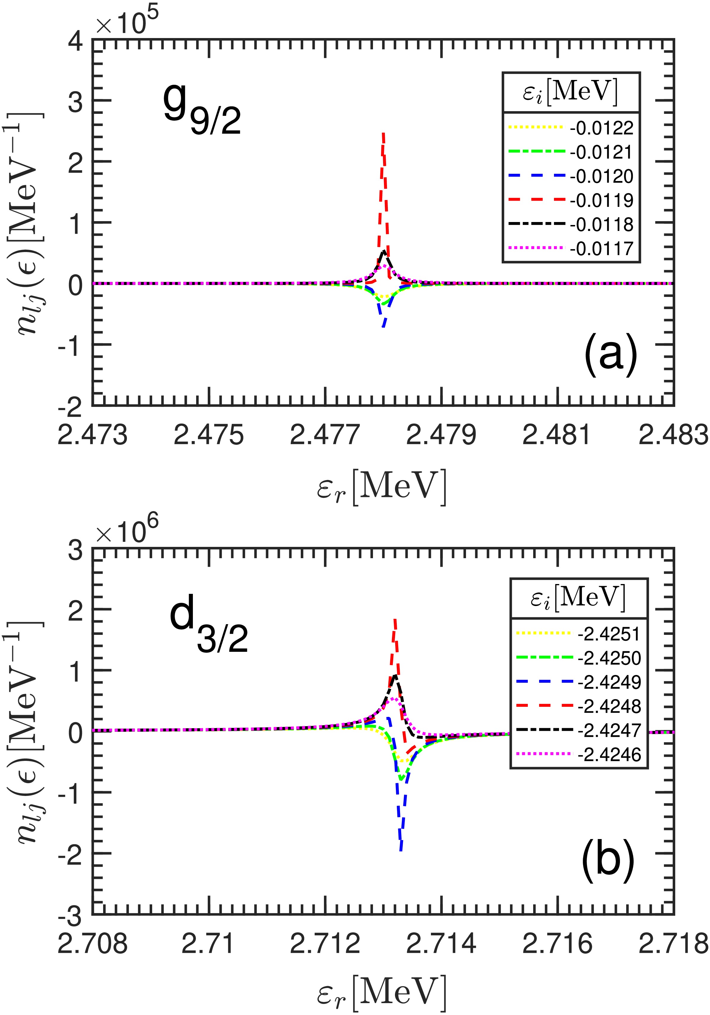

Figure 4.  (color online) The neutron DOSs $ n_{lj}(\epsilon)$ calculated with different real and imaginary parts of energy $ \varepsilon_r $ and $ \varepsilon_i $ in the coordinate space with $ R_{\text{box}} = 20 \, \text{fm} $ for (a) $ {g}_{9 / 2} $ and (b) $ {d}_{3 / 2} $ partial waves.

Following the same procedures, we can obtain the resonant energies and widths for all the other partial waves. In Table 2, the resonant energies and widths determined by the GFII method with different box sizes are listed for comparison. As is clearly seen, in comparison with those given by GFI, the results are less sensitive to the adopted box size. In particular, the GFII method with the box sizes $ R_{\rm box}=20 $ fm and 30 fm provides consistent results within an accuracy of $ 10^{-4} $ MeV for both narrow and broad resonances.

Inspired by the idea of the GFII method that the resonant states are identified by searching the extremes of DOSs, a more straightforward method was proposed in Refs. [59, 60] by probing the poles or extremes of the GF. To be more intuitive, one can integrate the modulus of GF $ \mathcal{G}_{lj}(r, r; \epsilon) $ over coordinate r

and search its extremes by scanning the real and imaginary parts ($ \varepsilon_r $, $ \varepsilon_i $) in the fourth quadrant of the complex energy plane. The resonant states will manifest themselves as peak structures at the resonant energy $ \varepsilon_R=\varepsilon_r $ with a width $ \Gamma=2\varepsilon_i $.

Taking the partial waves $ {g}_{9 / 2} $ and $ {d}_{3 / 2} $ as examples, Fig. 5 shows the 3-dimensional plot of the integral $ G_{lj}(\epsilon) $ as a function of the real and imaginary parts of energies $ \varepsilon_r $ and $ \varepsilon_i $ calculated with the box size $ R_{\rm box}=20 $ fm. In both panels, the peak structure representing the pole is obvious for the narrow resonance in $ {g}_{9 / 2} $ and the broad resonance in $ {d}_{3 / 2} $. From the peak structures, it is easy to identify the resonant energies and widths at the center of the peak, which are $ \varepsilon_R=\varepsilon_r=2.4780 $ MeV and $ \Gamma=-2\varepsilon_i=0.0238 $ MeV for the $ g_{9/2} $ partial wave, and $ \varepsilon_R=\varepsilon_r=2.7133 $ MeV and $ \Gamma=-2\varepsilon_i=4.8496 $ MeV for the $ d_{3/2} $ partial wave.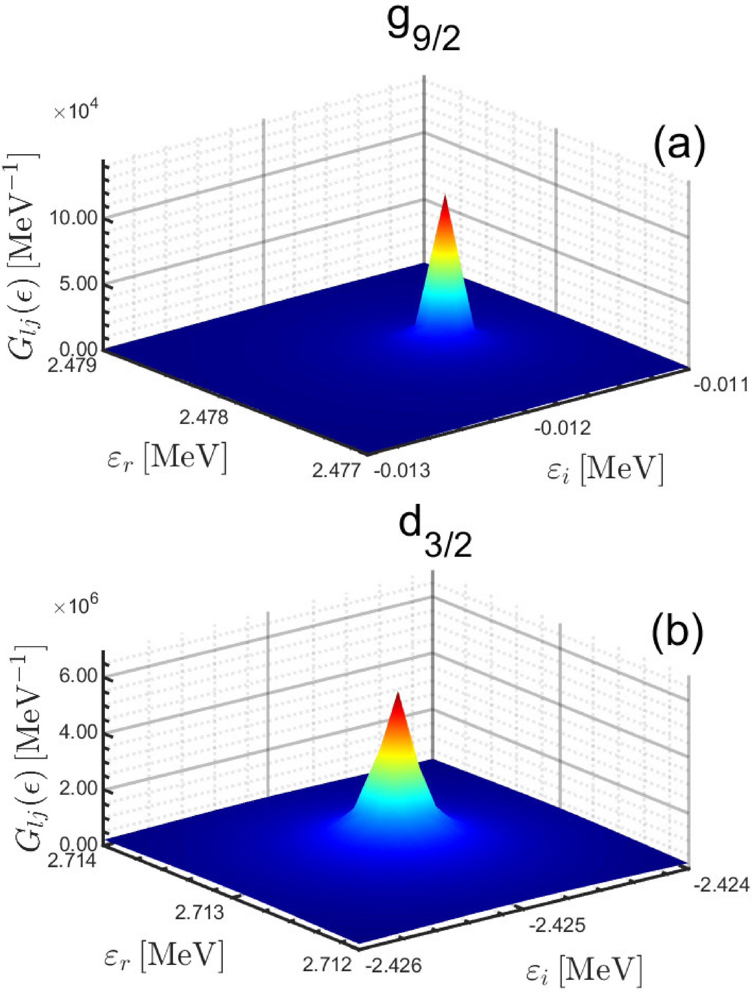

Figure 5.  (color online) Three-dimensional modulus $ G_{lj}(\epsilon) $ calculated with different real and imaginary parts of energy $ \varepsilon_r $ and $ \varepsilon_i $, in the coordinate space with $ R_{\rm{box}}=20\ \mathrm{fm} $ for (a) $ {g}_{9 / 2} $ and (b) $ {d}_{3 / 2} $ partial waves.

The GFIII method has been applied for all the partial waves calculated with different box sizes and the obtained resonant energies and widths are also listed in Table 2. As is clearly seen, the GFIII method is as effective as the GFII method and both methods are less sensitive to the adopted box size than the GFI method.

In Table 2, we have listed the single-neutron resonant energies $ \varepsilon_R $ and widths Γ for different partial waves in $ ^{40} $Ca obtained by the three methods GFI, GFII, and GFIII. To check the dependence on the box sizes, the calculations are carried out with different box sizes $ R_{\rm box}=10 $, 20, and 30 fm and the same mesh size $ \mathrm{d}r=0.1 $ fm. For comparison, the corresponding results obtained by the SM method [13] are also included.

For the resonant state in the partial wave $ g_{9/2} $ with small width, the methods GFI, GFII, and GFIII provide almost the same results as SM, which are also not much dependent on the box sizes. While for other partial waves which have relatively broad resonances, with the same box size, the results given by GFI are not much consistent with other methods. But, the results given by GFII and GFIII for these broad resonances are consistent with those obtained by SM. Furthermore, the results of GFII, GFIII and SM are not sensitive to the box sizes for these broad resonances.

In order to further check the results' dependence on the box sizes, one can plot the partial wave density distribution at the resonant energy $ \varepsilon_R $

Taking the narrow and broad resonances in partial waves $ g_{9/2} $ and $ d_{3/2} $ as examples, Fig. 6 shows their density distributions at the corresponding resonant energies $ \varepsilon_R $ calculated with box sizes $ R_{\rm box}=10, 20, 30 $ fm. As shown in Table 2, the resonant energies obtained by GFI, GFII, and GFIII are the same $ \varepsilon_R=2.478 $ MeV for the $ 1g_{9/2} $ resonant state. For the $ 2d_{3/2} $, the resonant energy obtained by GFI is different from those by GFII and GFIII. The resonant energies obtained by GFII and GFIII are consistent, i.e., $ \varepsilon_R=2.7143 $ MeV with $ R_{\rm box}=10 $ fm, and $ \varepsilon_R=2.7133 $ MeV with $ R_{\rm box}=20, 30 $ fm. We use these two resonant energies to plot the density distributions for $ 2d_{3/2} $ obtained with different box sizes correspondingly. It is obvious to see from Fig. 6 (a) that, the density distribution of narrow resonant state in $ g_{9/2} $ partial wave behaves as a bound state. Its density distribution decreases quickly to be zero after $ r\approx 8 $ fm. On the other hand, the broad resonance state in $ d_{3/2} $ partial wave in Fig. 6 (b) has obvious oscillating density distributions. However, for both narrow and broad resonances, the density distributions calculated by the GF method at their resonant energies are not sensitive to the box size. Especially for the broad resonant state in $ d_{3/2} $ partial wave with the rapid oscillations in the density distribution, even with the small box size $ R_{\rm box}=10 $ fm, it can still give consistent density distributions with those obtained by the larger boxes up to $ r=10 $ fm. The larger box sizes just display the density distribution in further region. This is just attributed to the proper description of the wave functions for the continuum states given by the GF method. This can also explain why the resonant energies and widths are not sensitive to the box sizes given by the GFII and GFIII methods. It is expected that, the density distributions calculated with GF can properly include the contributions from the continuum states in the density functional theory.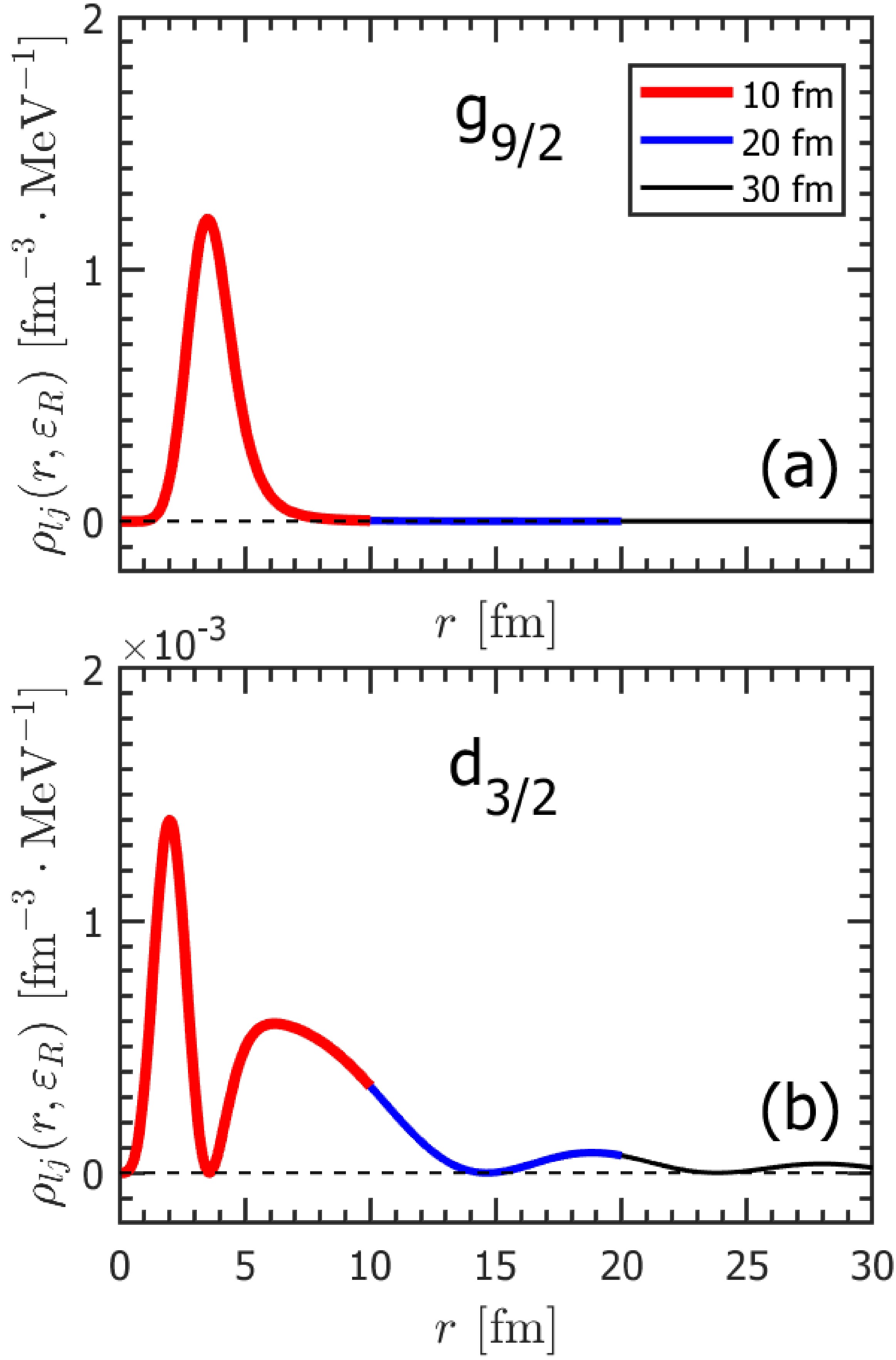

Figure 6.  (color online) Density distributions $ \rho_{lj}(r, \varepsilon_R) $ at the resonant energies $ \varepsilon_R $ for single-neutron resonant state (a) $ 1{g}_{9/2} $ and (b) $ 2{d}_{3 / 2} $ calculated in the coordinate space with box sizes $ R_{\mathrm{box}}=10, 20, 30\ \rm{fm} $ and the same mesh size $ 0.1\ \mathrm{fm} $.

Comparing the three methods GFI, GFII, and GFIII to provide the resonant energies and widths, the GFI method reading from the DOSs calculated with a fixed small imaginary part energy, is only reliable for the narrow resonant states. In contrast, the GFII and GFIII methods which scan the poles of the DOSs and the GF with different real and imaginary part of energies are reliable for both the narrow and resonant states. In practice, one can use GFI in the first step to locate the resonant states roughly, and then use GFII or GFIII to scan the poles around this location with a higher precision.

In this paper, the Schrödinger equation with Woods-Saxon type potentials for neutrons in $ ^{40}\mathrm{Ca} $ is solved by the GF method. The bound and resonant states are obtained with the GF constructed by the wave functions with proper boundary conditions corresponding to their energies. The GF results for both bound and resonant single-neutron states are consistent with those obtained by the shooting and SM methods. Explicitly, three different recipes (GFI, GFII, and GFIII) are used to figure out the energies and widths of resonant states. In the GFI method, by subtracting the contributions of free particle from the total DOS, one can identify the resonant states and obtain the corresponding energy and width information. In the GFII method, the resonant states are identified by the flip of DOS as the imaginary part of energy changes. More straightforwardly, in the GFIII method, the resonant states are identified as poles of the modulus of GF scanned in the fourth quadrant of the complex energy plane. Compared with the results given by the SM, it's found that GFI is only reliable for the narrow resonant states, while GFII and GFIII are effective for both the narrow and broad ones. It's also found that the energies, widths, and density distributions of resonant states obtained by the GF method exhibit a rather weak dependence on the box size. It is expected that the GF can provide the proper density distributions with the contributions from the continuum states in the density functional theory.