


 Abstract
 HTML
HTML Reference
 Related
 PDF
PDF


-
Recently, a near-threshold peaking structure
$ X(3960) $ was observed in the$ D_s^+D_s^- $ invariant mass distribution in the decay$ B^+\to D_s^+D_s^-K^+ $ by the LHCb Collaboration [1]. The measured mass and width were$ M=3956\pm5\pm10 $ MeV and$ \Gamma=43\pm13\pm8 $ MeV, respectively. Its quantum numbers$ J^{PC}=0^{++} $ are favored over$ 1^{–} $ and$ 2^{++} $ . The LHCb analysis indicates that this structure is an exotic candidate consisting of the$ cs\bar{c}\bar{s} $ constituent. In the same process, the LHCb also reported evidence of another structure,$ X_0(4140) $ , with mass$ 4133\pm6\pm6 $ MeV, width$ \Gamma=67\pm 17\pm7 $ MeV, and quantum numbers$ J^{PC}=0^{++} $ .Before the observation of
$ X(3960) $ , exotic states having the$ cs\bar{c}\bar{s} $ quark component have been reported in the$ J/\psi\phi $ invariant mass distributions by various experimental collaborations. In 2008, the CDF Collaboration first announced the evidence of a structure with mass$M= 4143.0\pm2.9\pm1.2$ MeV and width$ \Gamma= 11.7^{+8.3}_{-5.0}\pm3.7 $ MeV in the decay$ B^{+}\to J/\psi\phi K^{+} $ , named as$ X(4140) $ [2]. Later, the CMS Collaboration [3] and D0 Collaboration [4] confirmed the evidence of$ X(4140) $ in the same process; however, the Belle Collaboration [5], BABAR Collaboration [6], and LHCb Collaboration [7] did not obtain positive results for this state. From an analysis of the process$ \gamma\gamma\to J/\psi\phi $ [8], Belle obtained a narrow structure$ X(4350) $ with mass$ M=4350.6^{+4.6}_{-5.1}\pm0.7 $ MeV and width$\Gamma= 13^{+18}_{-9} \pm4$ MeV. In the decay$ B\to J/\psi\phi K $ , the CDF observed the evidence of a second$ J/\psi\phi $ structure with mass$M= 4274^{+8.4}_{-6.7}\pm1.9$ MeV and width$ \Gamma=32.3^{+21.9}_{-15.3}\pm7.6 $ MeV [9] while CMS reported the evidence with mass$M=4313.8 \pm5.3\pm7.3$ MeV and width$ \Gamma=38^{+30}_{-15}\pm15 $ MeV [3, 10]. With more collected data, LHCb Collaboration searched again for$ J/\psi\phi $ structures in the decay$ B^+\to J/\psi\phi K^+ $ [11]. This Collaboration confirmed the evidence of$ X(4140) $ with a broader width whose quantum numbers are determined to be$ J^{PC}=1^{++} $ . They also established the existence of$ X(4274) $ with$ J^{PC}=1^{++} $ and observed two higher resonances,$ X(4500) $ and$ X(4700) $ , with$ J^{PC}=0^{++} $ . In an improved analysis of$ B^+\to J/\psi\phi K^+ $ [12], the LHCb Collaboration observed two more states, namely$ X(4685) $ and$ X(4630) $ . The quantum numbers for the former state are$ J^P=1^+ $ while the preferred$ J^P $ for the latter are$ 1^- $ .Since the observation of
$ X_1(4140) $ 1 , various theoretical explanations such as compact$ cs\bar{c}\bar{s} $ tetraquarks and$ D_s^{*+}D_s^{*-} $ molecules have been proposed to understand the aforementioned exotic resonances in different methods [13−55]. Because of their high masses,$ X(4500) $ ,$ X(4700) $ ,$ X(4685) $ , and$ X(4630) $ may be interpreted as the orbitally or radially excited tetraquark or molecular states [19, 27, 32−38]. For$ X_1(4140) $ and$ X(4274) $ , the measured quantum numbers$ J^{PC}=1^{++} $ [12] do not support their$ D_s^{*+}D_s^{*-} $ molecule interpretation. For the newly observed$ X(3960) $ , the authors of Ref. [44−46] interpreted it as a hadronic molecule in the coupled$ D\bar{D}-D_s^+D_s^- $ system. Calculations based on the QCD sum rule method [47, 48] and one-boson-exchange model [49] also favor the molecule interpretation. Another calculation based on the QCD two-point sum rules [50] leads to the assignment of$ X(3960) $ as a scalar diquark-antidiquark state. From investigations on the$ D_s^+D_s^- $ invariant mass spectrum and ratio$ \Gamma(X\to D^+D^-)/\Gamma(D_s^+D_s^-) $ , Ref. [51] proposed that$ X(3960) $ is induced by the$ \chi_{c0}(2P) $ charmonium below the$ D_s^+D_s^- $ threshold. A combined analysis in Ref. [52] based on the assumption that$ X(3930) $ ,$ X(3960) $ , and$ X(3915) $ are the same hadron indicates that this state probably has a$ c\bar{c} $ core strongly renormalized by$ D_s^+D_s^- $ coupling. In Ref. [53],$ X(3960) $ and$ X_0(4140) $ are interpreted as four-quark$ cs\bar{c}\bar{s} $ states. Meanwhile, the conclusion that$ X_0(4140) $ is a$ D_s^+D_s^- $ molecule is drawn in [54]. The investigation in an improved chromomagnetic interaction model indicates that both$ X(3960) $ and$ X_0(4140) $ may be interpreted as$ 0^{++} \;\; cs\bar{c}\bar{s} $ tetraquark states [55].To understand the near-threshold structures
$ X(3960) $ and$ X_0(4140) $ and consider other possible tetraquark states, it is worthwhile to further study the$ cs\bar{c}\bar{s} $ tetraquark states systematically. In our previous study [13], we investigated the spectrum of$ cs\bar{c}\bar{s} $ states with a color-magnetic interaction (CMI) model. In this spectrum, there are two$ J^{PC}=1^{++} $ and four$ J^{PC}=0^{++} $ states. Our results indicate that$ X_1(4140) $ and$ X(4274) $ can be interpreted as these two axial-vector tetraquarks while$ X(4350) $ can be assigned as the highest scalar tetraquark. To gain more information about multiquark states, their decay properties must be investigated. We aimed to describe the rearrangement decays of hidden-charm pentaquark states [56, 57] and tetraquark states with different flavors [58] in a simple scheme, adopting the constant Hamiltonian$ H_{\rm decay}={\cal C} $ . In the present study, we continued our previous study on compact$ cs\bar{c}\bar{s} $ states by including the decay properties. We identify$ X_1(4140) $ as the low$ 1^{++} $ or$ X(4274) $ as the high$ 1^{++} \;\; cs\bar{c}\bar{s} $ tetraquark and use their masses and widths as inputs to discuss the masses and widths of$ cs\bar{c}\bar{s} $ states.This paper is organized as follows. In Section II, we present the CMI Hamiltonian, wave functions, and method to consider rearrangement decays. In Section III, we report on the model parameters and numerical results. The last section is devoted to discussion and summary.
-
The effective Hamiltonian in the CMI model to study the mass spectrum of the
$ cs\bar{c}\bar{s} $ tetraquark states reads$ H=\sum\limits_i m_i+H_{\mathrm{CMI}}=\sum\limits_i m_i-\sum\limits_{i<j}C_{ij} \lambda_i\cdot\lambda_j\sigma_i\cdot\sigma_j $

(1) where
$ m_i $ is effective mass of the i-th quark and$ C_{ij} $ denotes the effective coupling constant between the i-th and j-th quarks;$ \lambda_i $ and$ \sigma_i $ represent the$ S U(3)$ Gell-Mann and$S U(2) $ Pauli matrices for the i-th quark, respectively; for an antiquark,$ \lambda_i\to -\lambda_i^* $ . The mass splittings between different$ cs\bar{c}\bar{s} $ states are mainly induced by the term$ H_{\mathrm{CMI}} $ . The CMI model is a simplified quark model where$ m_i $ contains the constituent quark mass and contributions from the kinetic energy, color-Coulomb, and linear confinement terms.After obtaining the eigenvalue
$ E_{\mathrm{CMI}} $ of$ H_{\mathrm{CMI}} $ , the mass formula for a tetraquark state is obtained as follows:$ M =\sum\limits_i m_i+E_{\mathrm{CMI}}. $

(2) According to numerical results for various systems [13, 58−63], the estimated masses of either conventional hadrons or multiquark states obtained from this equation are higher than the measured values. The main reason is that the values of effective mass
$ m_i $ in different systems should indeed be different. This indicates that the effective attraction between quark components is not appropriately taken into consideration. These overestimated values can be regarded as theoretical upper limits for the multiquark masses. To reduce the uncertainties in the CMI model, the color-electric term must be included explicitly. Here, we use the following modified formula to explore the mass splittings between different$ cs\bar{c}\bar{s} $ states by introducing a reference system:$ \begin{array}{*{20}{l}} M =[M_{\rm ref}-(E_{\mathrm{CMI}})_{\rm ref}]+E_{\mathrm{CMI}}, \end{array} $

(3) where
$M_{\rm ref}$ and$(E_{\mathrm{CMI}})_{\rm ref}$ denote the measured mass and calculated CMI eigenvalue for the reference system, respectively. A meson-meson state may be adopted as a reference whose quark content is the same as the considered tetraquark; still, it is difficult to make a reasonable choice. In Ref. [13], we estimated the masses of$ cs\bar{c}\bar{s} $ tetraquarks using the$ J/\psi\phi $ and$ D^{+}_sD^{*-}_s $ thresholds and found that the resulting$ 1^{++} $ tetraquark masses in both cases were lower than the experimental measurements. The results with$ J/\psi\phi $ were approximately 100 MeV lower than those with$ D^{+}_sD^{*-}_s $ . Therefore, we may treat these underestimated values as lower limits for theoretical$ cs\bar{c}\bar{s} $ masses. By contrast,$ X_1(4140) $ is chosen as the reference state by assigning it to be the lower$ 1^{++} \;\; cs\bar{c}\bar{s} $ tetraquark, the assignment for$ X(4274) $ as the higher$ 1^{++} \;\; cs\bar{c}\bar{s} $ is acceptable. Following this line, we have extended studies using$ X_1(4140) $ as input to other tetraquark systems [58, 60]. In the present study, we kept working on this idea to update previous results [13] by including the decay information. For this purpose, it is necessary to know the spin$ \otimes $ color wave functions.For a
$ cs\bar{c}\bar{s} $ tetraquark, the total wave function is not constrained by the Pauli principle; however, one must consider its C-parity because it is a truly neutral state. We reported the spin$ \otimes $ color wave functions in Ref. [13] in the diquark-antidiquark base. For convenience, we present here the definitions again. Using the notation$ [(cs)_{\mathrm{color}}^{\mathrm{spin}}(\bar{c}\bar{s})_{\mathrm{color}}^{\mathrm{spin}}]^{\mathrm{spin}} $ , they are$ \begin{array}{*{20}{l}} {J^{PC}=2^{++}}: \quad &\phi_1\chi_1=[(cs)_{6}^{1}(\bar{c}\bar{s})_{\bar{6}}^{1}]^{2},\quad \phi_2\chi_1=[(cs)_{\bar{3}}^{1}(\bar{c}\bar{s})_{3}^{1}]^{2};\\ {J^{PC}=0^{++}}:\quad &\phi_1\chi_3=[(cs)_{6}^{1}(\bar{c}\bar{s})_{\bar{6}}^{1}]^{0},\quad \phi_2\chi_3=[(cs)_{\bar{3}}^{1}(\bar{c}\bar{s})_{3}^{1}]^{0}, \\ &\phi_1\chi_6=[(cs)_{6}^{0}(\bar{c}\bar{s})_{\bar{6}}^{0}]^{0},\quad\phi_2\chi_6=[(cs)_{\bar{3}}^{0}(\bar{c}\bar{s})_{3}^{0}]^{0}; \end{array} $ 
(4) $ \begin{array}{*{20}{l}} {J^{PC}=1^{++}}:\quad &\phi_1\chi_+=\dfrac{1}{\sqrt{2}}\Big([(cs)_{6}^{1}(\bar{c}\bar{s})_{\bar{6}}^{0}]^{1}+[(cs)_{6}^{0}(\bar{c}\bar{s})_{\bar{6}}^{1}]^{1}\Big),\quad \phi_2\chi_+=\dfrac{1}{\sqrt{2}}\Big([(cs)_{\bar{3}}^{1}(\bar{c}\bar{s})_{3}^{0}]^{1}+[(cs)_{\bar{3}}^{0}(\bar{c}\bar{s})_{3}^{1}]^{1}\Big);\\ {J^{PC}=1^{+-}}:\quad &\phi_1\chi_-=\dfrac{1}{\sqrt{2}}\Big([(cs)_{6}^{1}(\bar{c}\bar{s})_{\bar{6}}^{0}]^{1}-[(cs)_{6}^{0}(\bar{c}\bar{s})_{\bar{6}}^{1}]^{1}\Big),\quad \phi_2\chi_-=\dfrac{1}{\sqrt{2}}\Big([(cs)_{\bar{3}}^{1}(\bar{c}\bar{s})_{3}^{0}]^{1}-[(cs)_{\bar{3}}^{0}(\bar{c}\bar{s})_{3}^{1}]^{1}\Big),\\ &\phi_1\chi_2=[(cs)_{6}^{1}(\bar{c}\bar{s})_{\bar{6}}^{1}]^{1},\quad \quad\quad\quad\quad\quad\quad\quad\quad\quad \phi_2\chi_2=[(cs)_{\bar{3}}^{1}(\bar{c}\bar{s})_{3}^{1}]^{1}. \end{array} $

(5) We do not include the explicit CMI matrices here. Ref. [13] includes the matrices with bases
$(\phi_1\chi_1, \phi_2\chi_1)^{\rm T}$ ,$(\phi_1\chi_+, \phi_2\chi_+)^{{\rm T}}$ ,$(\phi_1\chi_3, \phi_2\chi_3, \phi_1\chi_6, \phi_2\phi_6)^{\rm T}$ , and$(\phi_1\chi_2, \phi_2\chi_2, \phi_1\chi_-, \phi_2\chi_-)^{\rm T}$ for the$ J^{PC}=2^{++} $ ,$ 1^{++} $ ,$ 0^{++} $ , and$ 1^{+-} $ cases, respectively. -
To reflect the effective CMI between quark components in multiquark states, various K factors were introduced in Ref. [59]. Later, in Ref. [60], we calculated the K factors for the
$ cs\bar{c}\bar{s} $ states. With them, we argued that the highest$ 2^{++} $ , highest$ 1^{++} $ , and second highest$ 0^{++} $ states are probably more stable than other partners. Whether this argument is sound or not will be checked in the next section. The K factor between the i-th and j-th quark components is given by$ K_{ij}=\lim\limits_{\Delta C_{ij}\to 0}\frac{\Delta E_{\rm CMI}}{\Delta C_{ij}}\to \frac{\partial E_{\rm CMI}}{\partial C_{ij}}, $

(6) where
$ \Delta C_{ij} $ is the variation of an effective coupling constant and$\Delta E_{\rm CMI}$ is the corresponding variation of a multiquark mass. Now, the mass of a tetraquark state can be rewritten as$ M=[M_{\rm ref}-(E_{\rm CMI})_{\rm ref}]+\sum\limits_{i<j}K_{ij}C_{ij} $

(7) The sign of
$ K_{ij} $ reflects whether the effective CMI [63] between the i-th and j-th quark components is attractive ($ K_{ij}<0 $ ) or repulsive ($ K_{ij}>0 $ ).The strong decays of conventional hadrons involve the creation of at least one quark-antiquark pair at the quark level. A quark creation mechanism must be selected for the calculations. The
$ ^3P_0 $ model is usually adopted to study the two-body strong decays when a unique coupling constant is used. For strong decays of compact tetraquark states, the two-body decay patterns should be the dominant ones; however, they do not involve quark creations. In this study, we used a simple method to calculate the rearrangement decay widths of$ cs\bar{c}\bar{s} $ states; in this method, the quark-level Hamitonian for the decay is taken as a constant, i.e.,$H_{\rm decay}=\mathcal {C}$ . It means that the four quark components in different tetraquarks scatter to meson-meson states freely with equal coupling strength. This method has been applied to deal with decays of pentaquark [56, 57] and tetraquark states with four different flavors [58]. In principle, gluon exchanges would induce corrections to this simple model, but additional parameters are needed. At present, we assume that the rearrangement decays for all the$ cs\bar{c}\bar{s} $ tetraquark states can be described by this single constant$ {\cal C} $ . Given that there is only one parameter, the partial width ratio is a good quantity to test the model. If more experimental decay data are available, modifications of the decay Hamiltonian may be considered.In the adopted model, the width for a rearrangement decay channel is expressed as
$ \Gamma=\frac{\sqrt{(M^2-(m_1+m_2)^2)(M^2-(m_1-m_2)^2)}}{16\pi M^3}|\mathcal{M}|^2, $

(8) where M,
$ m_1 $ , and$ m_2 $ are the masses of the initial tetraquark and two final mesons, respectively. The decay amplitude$ \mathcal{M}=\langle initial|H_{\rm decay}|final \rangle $ is given by$ \mathcal{M}=\mathcal{C}\sum\limits_{ij}\alpha_i\beta_j $

(9) where
$ \alpha_i $ , employed in Eq. (10), are coefficients of the initial wave function in the bases presented in the last subsection, and$ \beta_j $ denotes coefficients of the final meson-meson wave function in the same bases. Regarding the initial states, their spin-color wave functions have the forms$ \begin{aligned}[b] \Psi(2^{++}) &= \alpha_1\phi_1\chi_1+ \alpha_2\phi_2\chi_1,\\ \Psi(1^{++}) &= \alpha_1\phi_1\chi_+ +\alpha_2\phi_2\chi_+,\\ \Psi(0^{++}) &= \alpha_1\phi_1\chi_3+ \alpha_2\phi_2\chi_3+\alpha_3\phi_1\chi_6+\alpha_4\phi_2\chi_6,\\ \Psi(1^{+-}) &= \alpha_1\phi_1\chi_2+\alpha_2\phi_2\chi_2+\alpha_3\phi_1\chi_-+\alpha_4\phi_2\chi_-, \end{aligned} $

(10) where the normalization condition
$ \sum _{i=1}|\alpha_i|^2=1 $ is always satisfied. The values of$ \alpha_i $ are obtained from the eigenvector of the corresponding tetraquark CMI matrix. We show them explicitly in Table 2. There are two types of rearrangement decays, namely$Q_1q_2\bar{Q}_3\bar{q}_4\to (Q_1\bar{Q}_3)_{1c} +(q_2\bar{q}_4)_{1c}$ and$ Q_1q_2\bar{Q}_3\bar{q}_4\to(Q_1\bar{q}_4)_{1c}+(q_2\bar{Q}_3)_{1c} $ . The values of$ \beta_j $ are obtained by recoupling the final meson-meson states into forms similar to those in Eq. (10). Given that we project out the initial bases from the final wave functions, the following recoupling formulas in the color space are needed:$ J^{PC} $ 

$\langle H_{\rm CMI} \rangle$ 

Eigenvalue Eigenvector $ \mathrm{Mass} $ 

Lower limits Upper limits $ 2^{++} $ 

$ \left(\begin{array}{cc}62.8&-4.2\\-4.2&83.4\end{array}\right) $ 

$ \left(\begin{array}{c}84.2\\ 62.0\end{array}\right) $ 

$ \left(\begin{array}{cc}\{-0.19,0.98\}\\ \{-0.98,-0.19\}\end{array}\right) $ 

$ \left(\begin{array}{c}4316.9\\ 4294.6\end{array}\right) $ 

$ \left(\begin{array}{c}4120.1\\ 4097.8\end{array}\right) $ 

$ \left(\begin{array}{c}4617.2\\ 4595.0\end{array}\right) $ 

$ 1^{++} $ 

$ \left(\begin{array}{cc}-22.5&-81.2\\ -81.2&17.3\end{array}\right) $ 

$ \left(\begin{array}{c}80.9\\ -86.2\end{array}\right) $ 

$ \left(\begin{array}{cc}\{0.62,-0.79\}\\ \{-0.79,-0.62\}\end{array}\right) $ 

$ \left(\begin{array}{c}4313.6\\ 4146.5\end{array}\right) $ 

$ \left(\begin{array}{c}4116.8\\ 3949.6\end{array}\right) $ 

$ \left(\begin{array}{c}4613.9\\ 4446.8\end{array}\right) $ 

$ 0^{++} $ 

$ \left(\begin{array}{cccc}-52.0&8.5&-3.5&140.6\\ 8.5&-203.6&140.6&-8.7\\-3.5&140.6&-73.6&0\\ 140.6&-8.7&0&36.8\end{array}\right) $ 

$ \left(\begin{array}{c}139.9\\16.3\\-154.2\\-294.5\end{array}\right) $ 

$\left(\begin{array}{cccc}\{0.59,-0.01,-0.02,0.81\}\\ \{-0.03,-0.54,-0.84,-0.00\}\\ \{-0.80,-0.06,0.06,0.59\}\\ \{0.07,-0.84,0.54,-0.05\}\end{array}\right)$ 

$ \left(\begin{array}{c}4372.6\\ 4249.0\\ 4078.5\\ 3938.2\end{array}\right) $ 

$ \left(\begin{array}{c}4175.7\\ 4052.2\\ 3881.6\\ 3741.4\end{array}\right) $ 

$ \left(\begin{array}{c}4672.9\\ 4549.3\\ 4378.8\\ 4238.5\end{array}\right) $ 

$ 1^{+-} $ 

$ \left(\begin{array}{cccc}-13.7&4.2&-12.0&25.5\\ 4.2&-107.9&25.5&-30.0\\ -12.0&25.5&-26.5&81.2\\ 25.5&-30.0&81.2&7.3\end{array}\right) $ 

$ \left(\begin{array}{c}75.3\\-7.5\\-65.8\\-142.9\end{array}\right) $ 

$ \left(\begin{array}{cccc}\{-0.14,0.04,-0.60,-0.79\}\\ \{0.94,-0.07,-0.33,0.08\}\\ \{-0.28,-0.66,-0.54,0.43\}\\ \{-0.16,0.74,-0.48,0.44\}\end{array}\right) $ 

$ \left(\begin{array}{c}4308.0\\ 4225.1\\ 4166.9\\ 4089.8\end{array}\right) $ 

$ \left(\begin{array}{c}4111.2\\ 4028.3\\3970.0\\3892.9\end{array}\right) $ 

$ \left(\begin{array}{c}4608.3\\4525.5\\4467.2\\4390.1\end{array}\right) $ 

Table 2. Numerical results for the masses of
$ cs\bar{c}\bar{s} $ states in units of MeV. The bases for$\langle H_{\rm CMI}\rangle$ in the$ 2^{++} $ ,$ 1^{++} $ ,$ 0^{++} $ , and$ 1^{+-} $ cases are$(\phi_1\chi_1,\phi_2\chi_1)^{\rm T}$ ,$(\phi_1\chi_+,\phi_2\chi_+)^{\rm T}$ ,$(\phi_1\chi_3,\phi_2\chi_3,\phi_1\chi_6,\phi_2\chi_6)^{\rm T}$ , and$(\phi_1\chi_2,\phi_2\chi_2,\phi_1\chi_-,\phi_2\chi_-)^{\rm T}$ , respectively. The masses obtained with$ X_1(4140) $ are listed in the fifth column. The lower and upper limits for the masses are listed in the sixth and seventh columns, respectively.$ \begin{aligned}[b]& (Q_1\bar{Q}_3)_{1c}(q_2\bar{q}_4)_{1c}=-\frac{1}{\sqrt{3}}\phi_1+\sqrt{\frac{2}{3}}\phi_2,\\ &(Q_1\bar{q}_4)_{1c}(q_2\bar{Q}_3)_{1c}=\frac{1}{\sqrt{3}}\phi_1+\sqrt{\frac{2}{3}}\phi_2. \end{aligned} $

(11) In the spin space, similar formulas can be easily obtained by calculating the
$ 9j $ symbols. Then, explicit values of$ \beta_j $ are obtained with these two-space coefficients. -
The coupling parameters
$ C_{cs} $ ,$ C_{c\bar{s}} $ ,$ C_{c\bar{c}} $ , and$ C_{ss} $ that we adopt for estimating the$ cs\bar{c}\bar{s} $ masses are extracted from the measured masses of the conventional ground hadrons [64] by using their mass formulas in the CMI model. The relevant hadrons, values of their$ E_{\rm CMI} $ , and determined coupling parameters are listed in Table 1. Other coupling parameters are obtained in a similar manner [13, 60]. In Table 1, the errors of$ C_{ij} $ are also presented. Given that the systematic error of the CMI model cannot be estimated and it might be larger than the measurement error, we do not consider errors in the following numerical estimations. We just set$ C_{cs}=4.5 $ MeV,$ C_{c\bar{s}}=6.8 $ MeV,$ C_{c\bar{c}}=5.3 $ MeV, and$ C_{ss}=6.5 $ MeV. The adopted coupling parameters$ C_{cc} $ and$ C_{s\bar{s}} $ were obtained with the approximation$ \dfrac{C_{cc}}{C_{c\bar{c}}}= \dfrac{C_{ss}}{C_{s\bar{s}}}=\dfrac{C_{nn}}{C_{n\bar{n}}}\approx\dfrac23 $ . To estimate the upper limit masses, we used the effective quark masses$ m_s=(M_\Omega-8C_{ss})/3=542.4 $ MeV and$m_c=(3M_{\Sigma_c^*} -2M_\Delta-16C_{nc}+8C_{nn})/3=1724.1$ MeV, where n indicates u or d quark. The extraction details can be found in Refs. [13, 60]. To estimate the lower limits for the masses with the$ J/\psi\phi $ threshold,$ m_s $ and$ m_c $ are not required.Hadron $E_{\rm CMI}$ 

Hadron $E_{\rm CMI}$ 

$ C_{ij} $ 

$ \Xi_c^{\prime} $ 

$ \dfrac83C_{ns}-\dfrac{16}{3}C_{cn}-\dfrac{16}{3}C_{cs} $ 

$ \Xi_c^* $ 

$ \dfrac83C_{ns}+\dfrac{8}{3}C_{cn}+\dfrac{8}{3}C_{cs} $ 

$ C_{cs}=4.49\pm 0.08 $ 

$ D_s $ 

$ -16C_{c\bar{s}} $ 

$ D^*_s $ 

$ \dfrac{16}{3}C_{c\bar{s}} $ 

$ C_{c\bar{s}}=6.75\pm 0.02 $ 

$ \eta_c $ 

$ -16C_{c\bar{c}} $ 

$ J/\psi $ 

$ \dfrac{16}{3}C_{c\bar{c}} $ 

$ C_{c\bar{c}}=5.30\pm 0.02 $ 

$ 2\Omega+\Delta-(2\Xi^*+\Xi) $ 

$ 8C_{ss}+8C_{nn} $ 

$ (\Delta-N)/2 $ 

$ 8C_{nn} $ 

$ C_{ss}=6.46\pm 0.11 $ 

Table 1. Chromomagnetic interactions for relevant hadrons and obtained coupling parameters in units of MeV.
When the masses of other
$ cs\bar{c}\bar{s} $ states are estimated using$ X_1(4140) $ , the input mass needs to be determined. In Ref. [11], the mass and width of$ X_1(4140) $ determined by LHCb are$ 4146.5\pm 4.5^{+4.6}_{-2.8} $ MeV and$ 83\pm 21^{+21}_{-14} $ MeV, respectively. In Ref. [12], these values were updated to$ 4118\pm11^{+19}_{-36} $ MeV and$ 162\pm21^{+24}_{-49} $ MeV, respectively. In the particle data book [64], these values, averaged over different measurements, are$ 4146.5\pm 3.0 $ MeV and$ 19^{+7}_{-5} $ MeV, respectively. Although the experimental masses are all around 4140 MeV, the deviation in width is significant. For the other$ 1^{++} $ state, i.e.,$ X(4274) $ , the deviation in width between different collaborations is insignificant [64]. In Ref. [58], we used the LHCb results from Ref. [11] as inputs from a consistent consideration of widths between$ X_1(4140) $ and$ X(4274) $ . The necessary condition for our purpose is that$ \Gamma(X_1(4140)) $ and$ \Gamma(X(4274)) $ be comparable. Here, we still follow Ref. [58] and use data determined in Ref. [11]. The cases for other choices will also be discussed. In addition to using$ X_1(4140) $ as the reference state, we will also discuss the case using$ X(4274) $ as input.The rearrangement decay channels for a
$ 1^{++} \;\; cs\bar{c}\bar{s} $ state are$ J/\psi\phi $ and$ \dfrac{1}{\sqrt2}(D_s^{*+}D_s^–D_s^+D_s^{*-}) $ where the convention for a relative phase [65] is determined with$ D_s^{(*)+}=c\bar{s} $ and$ D_s^{(*)-}=s\bar{c} $ . Assuming that the total decay width of a tetraquark is equal to the sum of partial widths ($ \Gamma_{\rm sum} $ ) for rearrangement decay channels,$ \mathcal{C}=72822 $ MeV is extracted from the LHCb data [11].The final states for the decay of
$ cs\bar{c}\bar{s} $ tetraquarks involve conventional mesons containing the$ s\bar{s} $ component. In the quark model, the quark content of the vector meson ϕ is approximately$ s\bar{s} $ , but this is not the case for the content of the pseudoscalar mesons η and$ \eta^\prime $ . They are superpositions of the$ S U(3) $ singlet state$ \eta_1 $ and octet state$ \eta_8 $ ,$ \begin{aligned}[b] |\eta\rangle&={\rm cos}(\theta)|\eta_8\rangle-{\rm sin}(\theta)|\eta_1\rangle ,\\ |\eta^\prime\rangle&={\rm sin}(\theta)|\eta_8\rangle+{\rm cos}(\theta)|\eta_1\rangle, \end{aligned} $

(12) where θ is the mixing angle. We employed the value
$ \theta=-11.3^{\circ} $ [64] in our calculations.With the above parameters, we obtained numerical results for ground
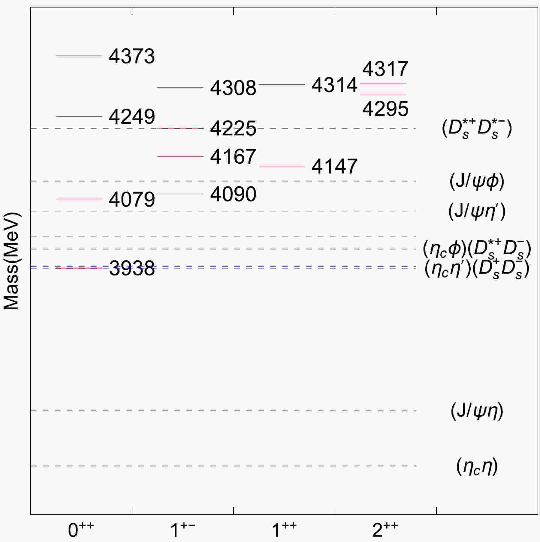
$ cs\bar{c}\bar{s} $ states. The mass results are presented in Table 2. Comparing with Ref. [13], there exist some differences in numbers; they mainly result from the variation of coupling parameters. We show the relative positions for the$ cs\bar{c}\bar{s} $ states using the input$ X_1(4140) $ in Fig. 1. The related meson-meson thresholds are also displayed. The results for the rearrangement decays are provided in Table 3.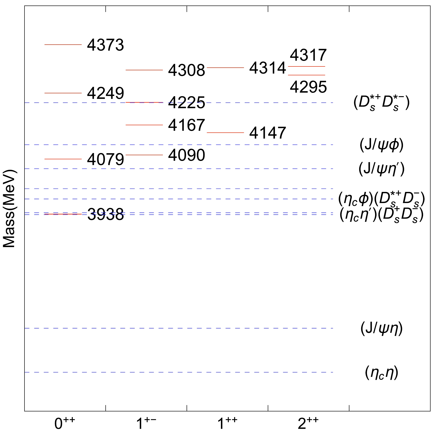
Figure 1. (color online) Relative positions for the
$ cs\bar{c}\bar{s} $ tetraquark states. The red solid and blue dashed lines correspond to estimated masses (with$ X_1(4140) $ ) and related meson-meson thresholds, respectively.$ J^{PC} $ 

Mass Channels $\Gamma_{\rm sum}$ 

$ J/ \psi \phi $ 

$ D_s^{*+}D_s^{*-} $ 

$ 2^{++} $ 

$ \left[\begin{array}{c}4316.9\\ 4294.6\end{array}\right] $ 

$ \left[\begin{array}{c}(83.4, 53.8)\\ (16.6, 10.2)\end{array}\right] $ 

$ \left[\begin{array}{c}(47.5, 23.9)\\ (52.5, 23.2)\end{array}\right] $ 

$ \left[\begin{array}{c}77.7\\ 33.4\end{array}\right] $ 

$ J/ \psi \phi $ 

$ (D_s^{*+}D_s^- - D_s^+D_s^{*-}) /\sqrt{2} $ 

$ 1^{++} $ 

$ \left[\begin{array}{c}4313.6\\ 4146.5\end{array}\right] $ 

$ \left[\begin{array}{c}(99.8, 63.9)\\ (0.2, 0.1)\end{array}\right] $ 

$ \left[\begin{array}{c}(8.2, 13.0)\\ (91.8, 82.9)\end{array}\right] $ 

$ \left[\begin{array}{c}76.9\\ 83.0\end{array}\right] $ 

$ J/ \psi \phi $ 

$ \eta_c \eta^{\prime} $ 

$ \eta_c \eta $ 

$ D_s^{*+}D_s^{*-} $ 

$ D_s^+D_s^- $ 

$ 0^{++} $ 

$ \left[\begin{array}{c}4372.6 \\ 4249.0\\ 4078.5\\ 3938.2\end{array}\right] $ 

$ \left[\begin{array}{c}(57.1, 40.9)\\ (39.5, 21.2)\\ (3.1, -)\\ (0.3, -)\end{array}\right] $ 

$ \left[\begin{array}{c}(0.0, 0.0)\\ (0.8, 0.7)\\ (18.0, 10.4)\\ (34.0, -)\end{array}\right] $ 

$ \left[\begin{array}{c}(0.0, 0.0)\\ (0.7, 0.8)\\ (16.0, 16.6)\\ (30.3, 28.2)\end{array}\right] $ 

$ \left[\begin{array}{c}(52.8, 32.9)\\ (42.7, 11.4)\\ (3.8, -)\\ (0.8, -)\end{array}\right] $ 

$ \left[\begin{array}{c}(0.1, 0.2)\\ (2.3, 2.2)\\ (49.2, 33.2)\\ (48.4, 3.6)\end{array}\right] $ 

$ \left[\begin{array}{c}74.0\\ 36.3\\ 60.2\\ 31.8\end{array}\right] $ 

$ J/ \psi \eta^{\prime} $ 

$ J/ \psi \eta $ 

$ \eta_c \phi $ 

$ D_s^{*+}D_s^{*-} $ 

$ (D_s^{*+}D_s^- + D_s^+D_s^{*-})/\sqrt{2} $ 

$ 1^{+-} $ 

$ \left[\begin{array}{c}4308.0\\ 4225.1\\ 4166.9\\ 4089.8\end{array}\right] $ 

$ \left[\begin{array}{c}(0.9, 0.6)\\ (3.0, 1.8)\\ (2.2, 1.1)\\ (46.9, 13.5)\end{array}\right] $ 

$ \left[\begin{array}{c}(0.8, 0.8)\\ (2.7, 2.7)\\ (1.9, 1.9)\\ (41.7, 38.2)\end{array}\right] $ 

$ \left[\begin{array}{c}(8.5, 6.9)\\ (36.8, 26.0)\\ (54.5, 33.8)\\ (0.2, 0.1)\end{array}\right] $ 

$ \left[\begin{array}{c}(97.7, 46.9)\\ (1.6, 0.1)\\ (0.1, -)\\ (0.6, -)\end{array}\right] $ 

$ \left[\begin{array}{c}(0.2, 0.4)\\ (23.4, 30.3)\\ (49.6, 50.8)\\ (26.8, 9.3)\end{array}\right] $ 

$ \left[\begin{array}{c}55.5\\ 60.9\\ 87.5\\ 61.0\end{array}\right] $ 

Table 3. Rearrangement decays for the
$ cs\bar{c}\bar{s} $ states resulting from assigning$ X_1(4140) $ as the lighter$ 1^{++} \;\; cs\bar{c}\bar{s} $ tetraquark. The numbers in parentheses are ($ 100|{\cal M}|^{2}/\mathcal{C}^{2},\Gamma $ ), where the coupling parameter$ \mathcal{C} $ is extracted from the width of$ X_1(4140) $ (83 MeV [11]). The partial width Γ and total width$\Gamma_{\rm sum}$ are expressed in units of MeV.Regarding the
$ 1^{++} \;\; cs\bar{c}\bar{s} $ states, their masses and decays were discussed in Refs. [13] and [58], respectively. Although the reported values are slightly different from those in Tables 2 and 3, the main conclusion is that$ X_1(4140) $ and$ X(4274) $ could be consistently interpreted as the two$ 1^{++} \;\; cs\bar{c}\bar{s} $ tetraquarks. The calculated$\Gamma_{\rm sum}=76.3$ MeV for the higher state is slightly larger than the measured width of$ 51\pm7 $ MeV [64]. It is worth noting that the adopted mass value of$ X(4274) $ (4313.6 MeV) is close to the CMS result ($ 4313.8\pm5.3\pm7.3 $ MeV) [3] but larger than the PDG result ($ 4286^{+8}_{-9} $ MeV) [64]. When one adopts the PDG value, the obtained$\Gamma_{\rm sum}$ is 10 MeV smaller, and closer to the measured width. According to Table 3, the width ratio between the two channels$ J/\psi\phi $ and$ D_s\bar{D}_s^* $ for the higher state is$ \Gamma(J/\psi\phi)/\Gamma(D_s^*\bar{D}_s)\simeq 4.9 $ , where$ D_s^*\bar{D}_s $ simply means the C-even$ D_s^{*+}D_s^{-}/D_s^{+}D_s^{*-} $ state, while that for the lower state is$ \Gamma(J/\psi\phi)/\Gamma(D_s^*\bar{D}_s)\simeq 10^{-3} $ . The hidden-charm decay for the$X_1(4140)$ is significantly suppressed.For the two
$ 2^{++} \;\; cs\bar{c}\bar{s} $ tetraquarks, their mass gap is 22.3 MeV. The higher state is broader than the lower one. The masses of both states are close to that of$ X(4274) $ determined by CMS [3]. If these two$ cs\bar{c}\bar{s} $ mesons do exist, the width ratio for the higher tetraquark between its two rearrangement decay channels is predicted to be$ \frac{\Gamma(J/\psi\phi)}{\Gamma(D_s^{*+}D_s^{*-})}\simeq 2.3, $

(13) and that for the lower tetraquark would be
$ \frac{\Gamma(J/\psi\phi)}{\Gamma(D_s^{*+}D_s^{*-})}\simeq 0.4. $

(14) These two values are different and the ratio can be used to uncover the nature of a
$ 2^{++} $ exotic state measured in future experiments. The mass gap between both tetraquarks is smaller than the width of any of them. It is also possible that only one state around 4.3 GeV be experimentally observed, but there are actually two states. The comparison of measurements in future experiments with the aforementioned width ratio between$ J/\psi\phi $ and$ D_s^{*+}D_s^{*-} $ will be helpful to understand possible structures of the observed state(s).In the case of
$ J^{PC}=0^{++} $ , there are four possible$ cs\bar{c}\bar{s} $ tetraquarks. The estimated mass of the highest state ($ 4372.6 $ MeV) is close to the mass of$ X(4350) $ . This result is consistent with the chiral quark model prediction of Ref. [14]. According to Table 3, the width of the highest state is approximately$ 74 $ MeV, which is larger than the width of$ X(4350) $ ($ 13^{+18}_{-9}\pm4 $ MeV). Note that the experimental value has a large uncertainty and we adopted a crude model. Future studies are still needed. At present, we can temporarily assign$ X(4350) $ as the highest$ cs\bar{c}\bar{s} $ tetraquark state with quantum numbers$ J^{PC}=0^{++} $ . In this case, our calculations indicate that its dominant decay channels are$ J/\psi\phi $ and$ D_s^{*+}D_s^{*-} $ , which could be used to test the assignment.The lowest
$ 0^{++} \;\; cs\bar{c}\bar{s} $ tetraquark has a mass of 3938.2 MeV and width of 31.8 MeV. It is a good candidate of the recently reported$ X(3960) $ . According to our results, this scalar tetraquark decays dominantly into the$ \eta_c\eta $ channel with the branching fraction Br$[X(3938.2)\to \eta_c\eta=89\%]$ . Although the coupling with the channel$ D_s^+D_s^- $ is also strong, the suppressed phase space results in a small partial width. With the assignment of$ X(3960) $ as the lowest scalar$ cs\bar{c}\bar{s} $ tetraquark state, we predict a decay ratio of$ \frac{\Gamma(\eta_c\eta)}{\Gamma(D_s^+D_s^-)}\simeq 7.8. $

(15) The search for
$ X(3960) $ in the$ \eta_c\eta $ and$ D_s^+D_s^- $ channels and check of this ratio can help better understand the nature of this exotic state.The mass and width of the second lowest
$ 0^{++} \;\; cs\bar{c}\bar{s} $ tetraquark are estimated to be$ 4078.5 $ MeV and$ 60.2 $ MeV, respectively, from our model. This mass is approximately 55 MeV smaller than that of$ X_0(4140) $ [1], but the width is consistent with that of$ X_0(4140) $ . If$ X_0(4140) $ can be interpreted as this$ cs\bar{c}\bar{s} $ tetraquark, the ratios between different partial widths are$ \begin{array}{*{20}{l}} \Gamma(\eta_c\eta^{\prime}):\Gamma(\eta_c\eta):\Gamma(D_s^+D_s^-)\simeq 1:1.6:3.2, \end{array} $

(16) which can be tested in future experiments.
The second highest
$ 0^{++} $ state has a mass of$ 4249.0 $ MeV and a width of$ 36.3 $ MeV. At present, no experimentally observed state can be related to this tetraquark, but its existence is possible. Although$ X(4274) $ has a similar mass and width, the quantum numbers are different. Further search for a$ cs\bar{c}\bar{s} $ state around 4250 MeV in the channel$ J/\psi\phi $ ,$ \eta_c\eta^{\prime} $ ,$ \eta_c\eta $ ,$ D_s^{*+}D_s^{*-} $ , or$ D_s^+D_s^- $ is strongly needed.In the
$ 1^{+-} $ case, there are four$ cs\bar{c}\bar{s} $ tetraquark states. According to Table 3, the widths of these states are all around 50$ - $ 90 MeV. For the lightest state, the coupling with the$ \eta_c\phi $ channel is weak and the corresponding partial width is extremely small. Therefore, this tetraquark has three dominant rearrangement decay channels. The width ratios between them are$ \begin{array}{*{20}{l}} \Gamma(J/\psi\eta^{\prime}): \Gamma(J/\psi\eta):\Gamma(D_s^*\bar{D}_s)\simeq 1.5:4.1:1.0, \end{array} $

(17) where
$ D_s^*\bar{D}_s $ simply means the C-odd$ D_s^{*+}D_s^-/D_s^+D_s^{*-} $ state. For the second lowest state, its mass is close to that of$ X_1(4140) $ . One may choose$ J/\psi\eta^{\prime} $ ,$ J/\psi\eta $ ,$ \eta_c\phi $ , and$ D_s^*\bar{D}_s $ to detect this tetraquark. Their dominant decay modes are$ \eta_c\phi $ and$ D_s^*\bar{D}_s $ and a ratio$ \Gamma(\eta_c\phi):\Gamma(D_s^*\bar{D}_s)\simeq 0.7 $ is predicted. For the second highest state, it is around the threshold of$ D_s^{*+}D_s^{*-} $ and has two dominant rearrangement decay modes, namely$ \eta_c\phi $ and$ D_s^*\bar{D}_s $ . The channels$ J/\psi\eta^{\prime} $ ,$ J/\psi\eta $ , and$ D_s^{*+}D_s^{*-} $ are suppressed. This tetraquark has similar properties to those of the second lowest one. For the highest state, which is around 4.3 GeV, it mainly decays into$ \eta_c\phi $ and$ D_s^{*+}D_s^{*-} $ with a ratio$\Gamma(\eta_c\phi): \Gamma(D_s^{*+}D_s^{*-})\simeq0.2$ . So far, no exotic states can be assigned as the$ 1^{+-} \;\; cs\bar{c}\bar{s} $ tetraquarks. Whether such states exist or not needs to be determined by future measurements. -
The above results were based on the assignment of
$ X_1(4140) $ as the lower$ 1^{++} \;\; cs\bar{c}\bar{s} $ tetraquark. Now, we analyze the case using the mass and width of$ X(4274) $ rather than$ X_1(4140) $ as inputs. Assuming that$ X(4274) $ with mass$ 4286^{+8}_{-9} $ MeV and width$ 51\pm 7 $ MeV [64] corresponds to the higher$ 1^{++} \;\; cs\bar{c}\bar{s} $ tetraquark, all the tetraquark masses in Table 2 would be 27.6 MeV lower. Table 4 lists the width results we obtained. All of them are smaller than those in Table 3. In this case, the mass of$ X_1(4140) $ is perfectly consistent with the updated value for the LHCb measurement [12], but the width is much smaller. The estimated mass of the lowest$ 0^{++} $ state is approximately 45 MeV smaller than the measured value of$ X(3960) $ [1]. The obtained width ($ 19.4 $ MeV) is also smaller than the measured value, i.e.,$ 43^{+15}_{-15} $ MeV. The second lowest$ 0^{++} $ state is approximately 82 MeV below the measured mass of$ X_0(4140) $ and its width is smaller than the measured one, which makes the interpretation of$ X_0(4140) $ as$ cs\bar{c}\bar{s} $ less reliable. The highest$ 0^{++} $ state has a mass closer to that of$ X(4350) $ than the previous case, but the width is still larger than the measured value. Comparing the possible tetraquark interpretations in the case using the LHCb results for$ X_1(4140) $ obtained in Ref. [11] with those of the case using$ X(4274) $ as the reference state, it is concluded that the former case provides a better description than the latter one.$ J^{PC} $ 

Mass Channels $ \Gamma_{sum} $ 

$ J/ \psi \phi $ 

$ D_s^{*+} D_s^{*-} $ 

$ 2^{++} $ 

$ \left[\begin{array}{c}4289.3\\ 4267.0\end{array}\right] $ 

$ \left[\begin{array}{c}(83.4, 35.6)\\ (16.6, 6.7)\end{array}\right] $ 

$ \left[\begin{array}{c}(47.5, 14.3)\\ (52.5, 12.9)\end{array}\right] $ 

$ \left[\begin{array}{c}49.9\\ 19.6\end{array}\right] $ 

$ J/ \psi \phi $ 

$ (D_s^{*+} D_s^- - D_s^+ D_s^{*-}) /\sqrt{2} $ 

$ 1^{++} $ 

$ \left[\begin{array}{c}4286.0\\ 4118.8\end{array}\right] $ 

$ \left[\begin{array}{c}(99.8, 42.3)\\ (0.2, 0.0)\end{array}\right] $ 

$ \left[\begin{array}{c}(8.2, 8.7)\\ (91.8, 45.2)\end{array}\right] $ 

$ \left[\begin{array}{c}51.0\\ 45.2\end{array}\right] $ 

$ J/ \psi \phi $ 

$ \eta_c \eta^{\prime} $ 

$ \eta_c \eta $ 

$ D_s^{*+} D_s^{*-} $ 

$ D_s^+D_s^- $ 

$ 0^{++} $ 

$ \left[\begin{array}{c}4345.0\\ 4221.4\\ 4050.9\\ 3910.6\end{array}\right] $ 

$ \left[\begin{array}{c}(57.1, 27.5)\\ (39.5, 13.5)\\ (3.1, -)\\ (0.3, -)\end{array}\right] $ 

$ \left[\begin{array}{c}(0.0, 0.0)\\ (0.8, 0.4)\\ (18.0, 6.6)\\ (34.0, -)\end{array}\right] $ 

$ \left[\begin{array}{c}(0.0, 0.0)\\ (0.7, 0.6)\\ (16.0, 11.5)\\ (30.3, 19.4)\end{array}\right] $ 

$ \left[\begin{array}{c}(52.8, 21.2)\\ (42.7, -)\\ (3.8, -)\\ (0.8, -)\end{array}\right] $ 

$ \left[\begin{array}{c}(0.1, 0.1)\\ (2.3, 1.5)\\ (49.2, 21.3)\\ (48.4, -)\end{array}\right] $ 

$ \left[\begin{array}{c}48.9\\ 16.0\\ 39.5\\ 19.4 \end{array}\right] $ 

$ J/ \psi \eta^{\prime} $ 

$ J/ \psi \eta $ 

$ \eta_c \phi $ 

$ D_s^{*+} D_s^{*-} $ 

$ (D_s^{*+} D_s^- + D_s^+ D_s^{*-})/\sqrt{2} $ 

$ 1^{+-} $ 

$ \left[\begin{array}{c}4280.4\\ 4197.5\\ 4139.2\\ 4062.1\end{array}\right] $ 

$ \left[\begin{array}{c}(0.9, 0.4)\\ (3.0, 1.2)\\ (2.2, 0.7)\\ (46.9, 4.4)\end{array}\right] $ 

$ \left[\begin{array}{c}(0.8, 0.6)\\ (2.7, 1.9)\\ (1.9, 1.3)\\ (41.7, 26.3)\end{array}\right] $ 

$ \left[\begin{array}{c}(8.5, 4.7)\\ (36.8, 17.4)\\ (54.5, 22.0)\\ (0.2, 0.1)\end{array}\right] $ 

$ \left[\begin{array}{c}(97.7, 27.4)\\ (1.6, -)\\ (0.1, -)\\ (0.6, -)\end{array}\right] $ 

$ \left[\begin{array}{c}(0.2, 0.2)\\ (23.4, 19.5)\\ (49.6, 30.0)\\ (26.8, -)\end{array}\right] $ 

$ \left[\begin{array}{c}33.3\\ 39.9\\ 53.9\\ 30.8 \end{array}\right] $ 

Table 4. Rearrangement decays for the
$ cs\bar{c}\bar{s} $ states resulting from assigning$ X(4274) $ as the higher$ 1^{++} \;\; cs\bar{c}\bar{s} $ tetraquark. The numbers in parentheses are ($ 100|{\cal M}|^{2}/\mathcal{C}^{2},\Gamma $ ), where the coupling parameter$ \mathcal{C} $ is extracted from the width of$ X(4274) $ (51 MeV [64]). The partial width Γ and total width$\Gamma_{\rm sum}$ are expressed in units of MeV.Up to now, we considered only one case for the mass and width of
$ X_1(4140) $ taken from Ref. [11]. We may also adopt the PDG values [64] or updated LHCb values [12] as inputs. Tables 5 and 6 show the obtained results in these two cases, respectively. The masses using the PDG values are the same as those in the last section, but the widths are much narrower. The width of the higher$ 1^{++} $ state is at least 26 MeV smaller than the PDG result for$ X(4274) $ . Although the width of the highest$ 0^{++} $ state is compatible with that of$ X(4350) $ , the width of the (second) lowest$ 0^{++} $ state is at least 20 (34) MeV smaller than that of$ X(3960) $ ($ X_0(4140) $ ). Therefore, the tetraquark picture using the PDG values is not as good as the case considered in the last section. In the case using the updated LHCb values, the masses are approximately equal to those of the case using$ X(4274) $ as the reference state, but the widths are much larger. This feature of the width leads to an unacceptable interpretation for$ X(4274) $ ,$ X(3960) $ ,$ X_0(4140) $ , and$ X(4350) $ as$ cs\bar{c}\bar{s} $ tetraquarks.$ J^{PC} $ 

Mass Channels $\Gamma_{\rm sum}$ 

$ J/ \psi \phi $ 

$ D_s^{*+} D_s^{*-} $ 

$ 2^{++} $ 

$ \left[\begin{array}{c}4316.9\\ 4294.6\end{array}\right] $ 

$ \left[\begin{array}{c}(83.4, 12.3)\\ (16.6, 2.3)\end{array}\right] $ 

$ \left[\begin{array}{c}(47.5, 5.5)\\ (52.5, 5.3)\end{array}\right] $ 

$ \left[\begin{array}{c}17.8\\ 7.7\end{array}\right] $ 

$ J/ \psi \phi $ 

$ (D_s^{*+} D_s^- - D_s^+ D_s^{*-}) /\sqrt{2} $ 

$ 1^{++} $ 

$ \left[\begin{array}{c}4313.6\\ 4146.5\end{array}\right] $ 

$ \left[\begin{array}{c}(99.8, 14.6)\\ (0.2, 0.0)\end{array}\right] $ 

$ \left[\begin{array}{c}(8.2, 3.0)\\ (91.8, 19.0)\end{array}\right] $ 

$ \left[\begin{array}{c}17.6\\ 19.0\end{array}\right] $ 

$ J/ \psi \phi $ 

$ \eta_c \eta^{\prime} $ 

$ \eta_c \eta $ 

$ D_s^{*+} D_s^{*-} $ 

$ D_s^+ D_s^- $ 

$ 0^{++} $ 

$ \left[\begin{array}{c}4372.6\\ 4249.0\\ 4078.5\\ 3938.2\end{array}\right] $ 

$ \left[\begin{array}{c}(57.1, 9.4)\\ (39.5, 4.9)\\ (3.1, -)\\ (0.3, -)\end{array}\right] $ 

$ \left[\begin{array}{c}(0.0, 0.0)\\ (0.8, 0.2)\\ (18.0, 2.4)\\ (34.0, -)\end{array}\right] $ 

$ \left[\begin{array}{c}(0.0, 0.0)\\ (0.7, 0.2)\\ (16.0, 3.8)\\ (30.3, 6.5)\end{array}\right] $ 

$ \left[\begin{array}{c}(52.8, 7.5)\\ (42.7, 2.6)\\ (3.8, -)\\ (0.8, -)\end{array}\right] $ 

$ \left[\begin{array}{c}(0.1, 0.0)\\ (2.3, 0.5)\\ (49.2, 7.6)\\ (48.4, 0.8)\end{array}\right] $ 

$ \left[\begin{array}{c}16.9\\ 8.3\\ 13.8\\ 7.3 \end{array}\right] $ 

$ J/ \psi \eta^{\prime} $ 

$ J/ \psi \eta $ 

$ \eta_c \phi $ 

$ D_s^{*+} D_s^{*-} $ 

$ (D_s^{*+} D_s^- + D_s^+ D_s^{*-})/\sqrt{2} $ 

$ 1^{+-} $ 

$ \left[\begin{array}{c}4308.0\\ 4225.1\\ 4166.9\\ 4089.8\end{array}\right] $ 

$ \left[\begin{array}{c}(0.9, 0.1)\\ (3.0, 0.4)\\ (2.2, 0.2)\\ (46.9, 3.1)\end{array}\right] $ 

$ \left[\begin{array}{c}(0.8, 0.2)\\ (2.7, 0.6)\\ (1.9, 0.4)\\ (41.7, 8.7)\end{array}\right] $ 

$ \left[\begin{array}{c}(8.5, 1.6)\\ (36.8, 5.9)\\ (54.5, 7.7)\\ (0.2, 0.0)\end{array}\right] $ 

$ \left[\begin{array}{c}(97.7, 10.7)\\ (1.6, 0.0)\\ (0.1, -)\\ (0.6, -)\end{array}\right] $ 

$ \left[\begin{array}{c}(0.2, 0.1)\\ (23.4, 6.9)\\ (49.6, 11.6)\\ (26.8, 2.1)\end{array}\right] $ 

$ \left[\begin{array}{c}12.7\\ 13.9\\ 20.0\\ 14.0\end{array}\right] $ 

Table 5. Rearrangement decays for the
$ cs\bar{c}\bar{s} $ states resulting from assigning$ X_1(4140) $ as the lighter$ 1^{++} \;\; cs\bar{c}\bar{s} $ tetraquark. The numbers in parentheses are ($ 100|{\cal M}|^{2}/\mathcal{C}^{2},\Gamma $ ), where the coupling parameter$ \mathcal{C} $ is extracted from the PDG width of$ X_1(4140) $ (19 MeV [64]). The partial width Γ and total width$\Gamma_{\rm sum}$ are expressed in units of MeV.$ J^{PC} $ 

Mass Channels $\Gamma_{\rm sum}$ 

$ J/ \psi \phi $ 

$ D_s^{*+}D_s^{*-} $ 

$ 2^{++} $ 

$ \left[\begin{array}{c}4288.4\\ 4266.1\end{array}\right] $ 

$ \left[\begin{array}{c}(83.4,128.8)\\ (16.6, 24.2)\end{array}\right] $ 

$ \left[\begin{array}{c}(47.5, 51.5)\\ (52.5, 46.4)\end{array}\right] $ 

$ \left[\begin{array}{c}180.3\\ 70.6\end{array}\right] $ 

$ J/ \psi \phi $ 

$ (D_s^{*+} D_s^- - D_s^{+} D_s^{*-}) /\sqrt{2} $ 

$ 1^{++} $ 

$ \left[\begin{array}{c}4285.1\\ 4118.0\end{array}\right] $ 

$ \left[\begin{array}{c}(99.8,152.9)\\ (0.2, 0.0)\end{array}\right] $ 

$ \left[\begin{array}{c}(8.2, 31.5)\\ (91.8,162.0)\end{array}\right] $ 

$ \left[\begin{array}{c}184.3\\ 162.0\end{array}\right] $ 

$ J/ \psi \phi $ 

$ \eta_c \eta^{\prime} $ 

$ \eta_c \eta $ 

$ D_s^{*+}D_s^{*-} $ 

$ D_s^+ D_s^- $ 

$ 0^{++} $ 

$ \left[\begin{array}{c}4344.1\\ 4220.5\\ 4050.0\\ 3909.7\end{array}\right] $ 

$ \left[\begin{array}{c}(57.1, 99.6)\\ (39.5, 48.6)\\ (3.1, -)\\ (0.3, -)\end{array}\right] $ 

$ \left[\begin{array}{c}(0.0, 0.1)\\ (0.8, 1.6)\\ (18.0, 23.9)\\ (34.0, -)\end{array}\right] $ 

$ \left[\begin{array}{c}(0.0, 0.1)\\ (0.7, 2.1)\\ (16.0, 41.8)\\ (30.3, 70.3)\end{array}\right] $ 

$ \left[\begin{array}{c}(52.8, 76.5)\\ (42.7, -)\\ (3.8, -)\\ (0.8, -)\end{array}\right] $ 

$ \left[\begin{array}{c}(0.1, 0.4)\\ (2.3, 5.4)\\ (49.2, 77.0)\\ (48.4, -)\end{array}\right] $ 

$ \left[\begin{array}{c}176.7\\ 57.7\\ 142.7\\ 70.3 \end{array}\right] $ 

$ J/ \psi \eta^{\prime} $ 

$ J/ \psi \eta $ 

$ \eta_c \phi $ 

$ D_s^{*+} D_s^{*-} $ 

$ (D_s^{*+} D_s^- + D_s^+ D_s^{*-})/\sqrt{2} $ 

$ 1^{+-} $ 

$ \left[\begin{array}{c}4279.5\\ 4196.6\\ 4138.4\\ 4061.3\end{array}\right] $ 

$ \left[\begin{array}{c}(0.9, 1.5)\\ (3.0, 4.3)\\ (2.2, 2.4)\\ (46.9, 15.1)\end{array}\right] $ 

$ \left[\begin{array}{c}(0.8, 2.0)\\ (2.7, 6.8)\\ (1.9, 4.7)\\ (41.7, 95.3)\end{array}\right] $ 

$ \left[\begin{array}{c}(8.5, 16.9)\\ (36.8, 62.7)\\ (54.5, 79.4)\\ (0.2, 0.2)\end{array}\right] $ 

$ \left[\begin{array}{c}(97.7, 98.7)\\ (1.6, -)\\ (0.1, -)\\ (0.6, -)\end{array}\right] $ 

$ \left[\begin{array}{c}(0.2, 0.9)\\ (23.4, 70.3)\\ (49.6,107.8)\\ (26.8, -)\end{array}\right] $ 

$ \left[\begin{array}{c}119.9\\ 144.2\\ 194.2\\ 110.6 \end{array}\right] $ 

Table 6. Rearrangement decays for the
$ cs\bar{c}\bar{s} $ states resulting from assigning$ X_1(4140) $ as the lighter$ 1^{++} \;\; cs\bar{c}\bar{s} $ tetraquark. The numbers in parentheses are ($ 100|{\cal M}|^{2}/\mathcal{C}^{2},\Gamma $ ), where the coupling parameter$ \mathcal{C} $ is extracted from the updated LHCb width of$ X_1(4140) $ (162 MeV [12]). The partial width Γ and total width$\Gamma_{\rm sum}$ are expressed in units of MeV.Let us now analyze the width ratios mentioned in the last section. When comparing such ratios between the above mentioned four cases, it is found that the width ratio of a tetraquark is mainly affected by whether the tetraquark has the same channels. When the decay channels are the same in these cases, the width ratios are not affected much. When a channel is kinematically forbidden in some cases, the ratio changes accordingly. The involved
$ cs\bar{c}\bar{s} $ tetraquarks are the highest$ 0^{++} $ , second lowest$ 0^{++} $ , and highest$ 1^{+-} $ states.From the above discussions, the calculated masses and widths of
$ cs\bar{c}\bar{s} $ tetraquark states using the reference state$ X_1(4140) $ whose mass and width are determined in Ref. [11] are more reasonable than other cases. Given that the input width of$ X_1(4140) $ still has large uncertainty, the obtained tetraquark widths may be updated. As a model calculation to understand the properties of the observed exotic states, we considered only the$ cs\bar{c}\bar{s} $ component in the present study. In fact, a physical charmonium-like state is probably a mixture of$ c\bar{c} $ ,$ cn\bar{c}\bar{n} $ ($ n=u,d $ ), and$ cs\bar{c}\bar{s} $ components. The possible assignments discussed in the last section may be improved once the mixture configuration can be considered. In that case, one would probably find appropriate positions for more states such as$ X(3930) $ [66, 67].In a previous study [60], we presented the K factors for various
$ cs\bar{c}\bar{s} $ tetraquark states. According to those results, we argued that the highest$ 2^{++} $ , highest$ 1^{++} $ , and second highest$ 0^{++} $ state are probably more stable than other states. According to Table 3, the estimated decay widths do not always satisfy this feature. The reason is that the decay width of a tetraquark is affected by the coupling matrix element, phase space, and number of decay channels, while the K factors are just directly related to the coupling matrix elements [58].To summarize, we studied properties of the compact
$ cs\bar{c}\bar{s} $ tetraquark states in the present study. The masses and rearrangement decay widths were estimated under the assumption that$ X(4140) $ is the lower$ 1^{++} \;\; cs\bar{c}\bar{s} $ tetraquark. Our results show that the recently reported state$ X(3960) $ announced by the LHCb Collaboration [1] could be assigned as the lowest$ 0^{++} \;\; cs\bar{c}\bar{s} $ tetraquark, and$ X(4350) $ , observed by Belle [5], as the highest$ 0^{++} $ tetraquark. Our results also suggest that$ X_0(4140) $ may be a candidate for the second lowest$ 0^{++} \;\; cs\bar{c}\bar{s} $ tetraquark. The ratios between partial widths of dominant channels for these announced states were predicted. If all the compact$ cs\bar{c}\bar{s} $ tetraquarks exist, besides these five candidates, seven states are still awaiting to be observed. Four of them have quantum numbers$ J^{PC}=1^{+-} $ , two of them have$ J^{PC}=2^{++} $ , and one of them has$ J^{PC}=0^{++} $ . Possible finding channels for them are presented. Hopefully, these predictions will be confirmed by future experimental data .
X(3960), X0(4140), and other compact ${\boldsymbol c \boldsymbol s\bar{\boldsymbol c}\bar{\boldsymbol s}} $ states
- Received Date: 2024-01-07
- Available Online: 2024-06-15
Abstract: We studied the spectrum and rearrangement decays of S-wave


 DownLoad: