


 Abstract
 HTML
HTML Reference
 Related
 PDF
PDF


-
In 2012, a new boson of approximately
$ 125 \; {{\rm{GeV}}} $ was discovered at the LHC [1,2], which in later years, was consistently verified to be the SM-like Higgs boson with an increasing amount of data [3-7]. However, some other questions still exist, e.g., whether another scalar survives in the low mass region, and whether there is exotic Higgs decay into light scalars. Before the LHC, for the low integrated luminosity (IL), the LEP did not exclude a light scalar with a smaller production rate than the SM-like Higgs [8]. The CMS(ATLAS) collaboration searched for resonances directly in the$ bj\mu\mu $ channel in the$ 10\!\sim\!60 $ ($ 20\!\sim\!70 $ ) GeV range [9,10]. The two collaborations also searched for the exotic Higgs decay to light resonances in final states with$ b\bar{b}\tau^+\tau^- $ [11],$ b\bar{b}\mu^+\mu^- $ [12,13],$ \mu^+\mu^-\tau^+\tau^- $ [14-16],$ 4\tau $ [16,17],$ 4\mu $ [18-20],$ 4b $ [21],$ \gamma\gamma gg $ [22], and$ 4\gamma $ [23]. However, there is still sufficient space left for physics on the exotic decay. For example, in the$ b\bar{b}\tau^+\tau^- $ channel reported by CMS collaboration [11], the 95% exclusion limit is at least 3% in the$ 20\sim60 \; {{\rm{GeV}}} $ region. According to simulations, however, the future limits could be 0.3% at the High-Luminosity program of the Large Hadron Collider (HL-LHC) [24], 0.04% at the Circular Electron Positron Collider (CEPC), and 0.02% at the Future Circular Colliders in$ e^+e^- $ collisions (FCC-ee) [25, 26].This exotic Higgs decay to light scalars can be investigated via many theories beyond the Standard Model (BSM) [27], e.g., the next-to minimal supersymmetric standard model (NMSSM), the simplest little Higgs model, the minimal dilaton model, the two-Higgs-doublet model, the next-to two-Higgs-doublet model, the singlet extension of the SM, etc. Several phenomenological studies on the exotic decay exist with these models [28-42].
The NMSSM extends the MSSM by a singlet superfield
$ \hat{S} $ , thereby solving the$ \mu $ -problem and relaxing the fine-tuning tension resulting from the discovery of the Higgs in 2012 [43-49]. However, as supersymmetric (SUSY) models, the MSSM and NMSSM both suffer from a huge parameter space of over 100 dimensions. In most studies, some parameters are manually assumed equal at low-energy scales, leaving only about 10 free parameters, without considering the Renormalization Group Equations (RGEs) running from high scales [43-49]. In Ref. [33], decay of a Higgs boson of$ 125 \; {{\rm{GeV}}} $ into light scalars was studied in the NMSSM with parameters set in this way. In contrast, in constrained models, congeneric parameters are assumed universal at the Grand Unified Theoretical (GUT) scale, leaving only four free parameters in the fully-constrained MSSM (CMSSM) and four or five in the fully-constrained NMSSM (CNMSSM) [50-57]. However, it was found that CMSSM and CNMSSM were nearly excluded considering the$ 125 \; {{\rm{GeV}}} $ Higgs data, high mass bounds of gluino and squarks in the first two generations, muon g-2, and dark matter relic density and detections [56-62].The semi-constrained NMSSM (scNMSSM) relaxes the unified conditions of the Higgs sector at the GUT scale; thus, it is also called the NMSSM with non-universal Higgs mass (NUHM) [63-66]. It not only keeps the simplicity and grace of the CMSSM and CNMSSM but also relaxes the tension that they have faced since the discovery of SM-like Higgs [67]. Moreover, it makes predictions about interesting light particles such as a singlino-like neutralino [68] and light Higgsino-dominated NLSPs [69-71]. In this work, we study the scenarios in the scNMSSM with a light scalar of
$ 10\sim60 \; {{\rm{GeV}}} $ and the detections of exotic Higgs decay to a pair of it.The main points of this paper are listed as follows. In Sec. II, we introduce the model briefly and provide some related analytic formulas. In Sec. III, we present in detail the numerical calculations and discussions. Finally, we draw our conclusions in Sec. IV.
-
The superpotential of NMSSM, with
$ \mathbb{Z}_3 $ symmetry, is written as [72]$W = W_{\rm{Yuk}}+\lambda \hat{S} \hat{H}_{u}\cdot\hat{H}_{d}+\frac{1}{3}\kappa \hat{S}^3\,, $

(1) from which the so-called F-terms of the Higgs potential can be derived as
$ V_{\rm{F}} = |\lambda S|^2(|H_u|^2+|H_d|^2)+|\lambda H_u\cdot H_d+\kappa S^2|^2 \,. $

(2) The D-terms are the same as in the MSSM
$ V_{\rm{D}} = \frac{1}{8}\left(g_1^2+g_2^2\right)\left(|H_d|^2-|H_u|^2\right)^2 +\frac{1}{2}g_2^2\left|H^{\dagger}_u H_d\right|^2 \,, $

(3) where
$ g_1 $ and$ g_2 $ are the gauge couplings of$ U(1)_Y $ and$ SU(2)_L $ , respectively. Without considering the SUSY-breaking mechanism, at a low-energy scale, the soft-breaking terms can be imposed manually to the Lagrangian. In the Higgs sector, these terms corresponding to the superpotential are$ \begin{aligned}[b] V_{\rm{soft}} =& M^2_{H_u}|H_u|^2+M^2_{H_d}|H_d|^2+M^2_S|S|^2 \\ &+\left(\lambda A_{\lambda}SH_u\cdot H_d+\frac{1}{3}\kappa A_{\kappa}S^3+{\rm h.c.}\right) \,, \end{aligned} $

(4) where
$ M^2_{H_u},\, M^2_{H_u},\, M^2_{S} $ are the soft masses of Higgs fields$ H_u,\, H_d,\,S $ , respectively, and$ A_\lambda,\, A_\kappa $ are the trilinear couplings at the$ M_{\rm{SUSY}} $ scale. However, in the scNMSSM, the SUSY breaking is mediated by gravity; thus, the soft-parameters at the$ M_{\rm{SUSY}} $ scale are running naturally from the GUT scale complying with the RGEs.At electroweak symmetry breaking,
$ H_u $ ,$ H_d $ , and$ S $ get their vacuum expectation values (VEVs)$ v_u $ ,$ v_d $ , and$ v_s $ , respectively, with$ \tan\beta\equiv v_u/v_d $ ,$ v \equiv \sqrt{v_u^2+v_d^2}\approx 174 \; {{\rm{GeV}}} $ , and$ \mu_{\rm{eff}}\equiv \lambda v_s $ . Then, they can be written as$ \begin{aligned}[b] &H_u = \left( \begin{array}{c} H_u^+ \\ v_u+\dfrac{\phi_1+{\rm i}\varphi_1}{\sqrt{2}} \\ \end{array} \right), \\& H_d = \left( \begin{array}{c} v_d+\dfrac{\phi_2+{\rm i}\varphi_2}{\sqrt{2}} \\ H_d^- \\ \end{array} \right), \quad \\ &S = v_s+\frac{\phi_3+{\rm i}\varphi_3}{\sqrt{2}}. \end{aligned} $

(5) The Lagrangian consists of the F-terms, D-terms, and soft-breaking terms; therefore, with the above equations, one can get the tree-level squared-mass matrix of CP-even Higgses in the base
$ \{\phi_1, \phi_2, \phi_3\} $ and CP-odd Higgses in the base$ \{\varphi_1, \varphi_2, \varphi_3\} $ [72]. After diagonalizing the mass squared matrixes including loop corrections [73], one can get the mass-eigenstate Higgses (three CP-even ones$ h_{1,2,3} $ and two CP-odd ones$ a_{1,2} $ , in mass order) from the gauge-eigenstate ones ($ \phi_{1,2,3} $ and$ \varphi_{1,2,3} $ in Eq. (5), with$ 1,2,3 $ corresponding to up-type, down-type, and singlet states, respectively):$ \quad h_i = S_{ik}\, \phi_k, \quad a_j = P_{jk}\, \varphi_k \,, $

(6) where
$ S_{ik}, P_{jk} $ are the corresponding components of$ \phi_k $ in$ h_i $ and$ \varphi_k $ in$ a_j $ , respectively, with$ i,k = 1,2,3 $ and$ j = 1,2 $ .In the scNMSSM, the SM-like Higgs (hereafter, uniformly denoted as
$ h $ ) can be CP-even$ h_1 $ or$ h_2 $ , and the light scalar (hereafter uniformly denoted as$ s $ ) can be CP-odd$ a_1 $ or CP-even$ h_1 $ . Then, the couplings between the SM-like Higgs and a pair of light scalars$ C_{hss} $ can be written at tree level as [74]$ \begin{aligned}[b] C_{h_2h_1h_1}^{\rm{tree}} \! = \!& \frac{\lambda^2}{\sqrt{2}} \left[v_u\left(\Pi^{122}_{211}+\Pi^{133}_{211}\right) \right.\\ & \left. +v_d\left(\Pi^{211}_{211}+\Pi^{233}_{211}\right) +v_s\left(\Pi^{311}_{211}+\Pi^{322}_{211}\right) \right] \\ &-\frac{\lambda\kappa}{\sqrt{2}} \left(v_u\Pi^{323}_{211}+v_d\Pi^{313}_{211}+2v_s\Pi^{123}_{211}\right) \\ &+\sqrt{2}\kappa^2v_s \Pi^{333}_{211}-\frac{\lambda A_{\lambda}}{\sqrt{2}}\Pi^{123}_{211}+\frac{\kappa A_{\kappa}}{3\sqrt{2}}\Pi^{333}_{211} \\ &+\frac{g^2}{2\sqrt{2}} \left[v_u \left(\Pi^{111}_{211}-\Pi^{122}_{211}\right)-v_d \left(\Pi^{211}_{211}-\Pi^{222}_{211}\right) \right] \,, \end{aligned} $

(7) where
$ \Pi^{ijk}_{211} = 2S_{2i}S_{1j}S_{1k}+2S_{1i}S_{2j}S_{1k}+2S_{1i}S_{1j}S_{2k} \,; $

or
$ \begin{aligned}[b] C_{h_a a_1a_1}^{\rm{tree}} = &\frac{\lambda^2}{\sqrt{2}} \left[v_u \left(\Pi^{122}_{a11}+\Pi^{133}_{a11}\right) \right. \\ & \left. +v_d\left(\Pi^{211}_{a11}+\Pi^{233}_{a11}\right) +v_s\left(\Pi^{311}_{a11}+\Pi^{322}_{a11}\right) \right] \\ &+\frac{\lambda\kappa}{\sqrt{2}} \left[v_u\left(\Pi^{233}_{a11}-2\Pi^{323}_{a11}\right)+v_d \left(\Pi^{133}_{a11}-2\Pi^{313}_{a11}\right) \right. \\ &\left.+2v_s \left(\Pi^{312}_{a11}-\Pi^{123}_{a11}-\Pi^{213}_{a11}\right) \right.] +\sqrt{2}\kappa^2 v_s\Pi^{333}_{a11} \\ &+\frac{\lambda A_{\lambda}}{\sqrt{2}}\left(\Pi^{123}_{a11}+\Pi^{213}_{a11}+\Pi^{312}_{a11}\right)-\frac{\kappa A_{\kappa}}{3\sqrt{2}}\Pi^{333}_{a11} \\ &+\frac{g^2}{2\sqrt{2}} \left[v_u\left(\Pi^{111}_{a11}-\Pi^{122}_{a11}\right)-v_d \left(\Pi^{211}_{a11}-\Pi^{222}_{a11}\right) \right] \,, \end{aligned} $

(8) where
$ \Pi^{ijk}_{a11} = 2S_{ai}P_{1j}P_{1k} $ , and$ a = 1,2 $ . Thus, the width of Higgs decay to a pair of light scalars can be given by$ \Gamma(h\to s s) = \frac{1}{32\pi m_{h}}C^2_{hss}\left({1-\frac{4m^2_{s}}{m^2_h}}\right)^{1/2} \,. $

(9) Then, the light scalars decay to light SM particles, such as a pair of light quarks or leptons, gluons, or photons. The widths of light scalar decay to quarks and charged leptons at tree level are given by
$ \Gamma(s\to l^+l^-) = \frac{\sqrt{2}G_F}{8\pi}m_s m^2_l \left({1-\frac{4m^2_l}{m^2_s}}\right)^{p/2} \,,$

(10) $ \Gamma(s\to q \bar{q}) = \frac{N_c G_F}{4\sqrt{2}\pi}C^2_{s q q}m_s m^2_q \left({1-\frac{4m^2_q}{m^2_s}}\right)^{p/2} \,, $

(11) where
$ p = 1 $ for CP-odd$ s $ , and$ p = 3 $ for CP-even$ s $ . The couplings between light scalar and up-type or down-type quarks are given by$ C_{h_1t_L t^c_R} = \frac{m_t}{\sqrt{2}v \sin\beta}S_{11} \,, $

(12) $ C_{h_1b_L b^c_R} = \frac{m_b}{\sqrt{2}v \cos\beta}S_{12} \,, $

(13) $ C_{a_1t_L t^c_R} = {\rm i}\frac{m_t}{\sqrt{2}v \sin\beta}P_{11} \,, $

(14) $ C_{a_1b_L b^c_R} = {\rm i}\frac{m_b}{\sqrt{2}v \cos\beta}P_{12} \,. $

(15) -
In this work, we first scan the following parameter space with NMSSMTOOLS-5.5.2 [74,75]:
$ \begin{aligned}[b] &0\!<\!\lambda\!<\!0.7, \qquad 0\!<\!\kappa\!<\!0.7, \qquad 1\!<\!\tan\!\beta\!<\!30, \\ &100\!<\!\mu_{\rm{eff}}\!<\!200 \; {{\rm{GeV}}}, \qquad 0\!<\!M_0\!<\!500 \; {{\rm{GeV}}}, \\ &0.5\!<\!M_{1/2}\!<\!2 \; {\rm{TeV}}, \qquad |A_0|,\, |A_{\lambda}|,\, |A_{\kappa}|\!<\!10 \; {\rm{TeV}} \,, \qquad \end{aligned} $

(16) where we choose small
$ \mu_{\rm{eff}} $ to get low fine tuning, small$ M_0 $ to get large muon g-2, and moderate$ M_{1/2} $ to meet both large muon g-2 and high gluino-mass bounds. The regions of other parameters are chosen to be wide to investigate all scenarios with a low mass scalar and the exotic Higgs decay.The constraints we imposed in our scan include the following: (i) an SM-like Higgs of
$ 123\!\!\sim\!\!127 \; {{\rm{GeV}}} $ , with signal strengths and couplings satisfying the current Higgs data [3-7]; (ii) search results for exotic and invisible decay of the SM-like Higgs, and Higgs-like resonances in other mass regions, with HIGGSBOUNDS-5.7.1 [76-78]; (iii) the muon g-2 constraint, like that in Ref. [67]; (iv) the mass bounds of gluino and the first-two-generation squarks over$ 2 \; {\rm{TeV}} $ and search results for electroweakinos in multilepton channels [79]; (vi) the dark matter relic density$ \Omega h^2 $ below 0.131 [80], and the dark matter and nucleon scattering cross section below the upper limits in direct searches [81,82]; and (vii) the theoretical constraints of vacuum stability and Landau pole.After imposing these constraints, the surviving samples can be categorized into three scenarios:
• Scenario I:
$ h_2 $ is the SM-like Higgs, and the light scalar$ a_1 $ is CP-odd;• Scenario II:
$ h_1 $ is the SM-like Higgs, and the light scalar$ a_1 $ is CP-odd;• Scenario III:
$ h_2 $ is the SM-like Higgs, and the light scalar$ h_1 $ is CP-even.In Table 1, we list the ranges of parameters and light particle masses in the three scenarios. From the table, one can see that the parameter ranges are nearly the same except for
$ \lambda $ ,$ \kappa $ , and$ A_\kappa $ , but the mass spectrums for light particles are totally different.Scenario I Scenario II Scenario III $ \lambda $ 

$ 0\sim0.58 $ 

$ 0\sim 0.24 $ 

$ 0\sim 0.57 $ 

$ \kappa $ 

$ 0\sim0.21 $ 

$ 0\sim0.67 $ 

$ 0\sim0.36 $ 

$ \tan\beta $ 

$ 14\sim27 $ 

$ 10\sim28 $ 

$ 13\sim28 $ 

$\mu_{\rm{eff} }/{\rm{GeV} }$ 

$ 103\sim200 $ 

$ 102\sim200 $ 

$ 102\sim200 $ 

$M_0\;/ {\rm{GeV} }$ 

$ 0\sim500 $ 

$ 0\sim500 $ 

$ 0\sim500 $ 

$M_{1/2}/ {\rm{TeV}}$ 

$ 1.06\sim1.47 $ 

$ 1.04\sim1.44 $ 

$ 1.05\sim1.47 $ 

$A_0/ {\rm{TeV} }$ 

$ -2.8\sim0.2 $ 

$ -3.2\sim-1.0 $ 

$ -2.8\sim0.6 $ 

$A_{\lambda} (M_{\rm{GUT} })/ {\rm{TeV} }$ 

$ 1.3\sim9.4 $ 

$ 0.1\sim10 $ 

$ 1.1\sim9.8 $ 

$A_{\kappa}(M_{\rm{GUT} })/{\rm{TeV} }$ 

$ -0.02\sim5.4 $ 

$ -0.02\sim0.9 $ 

$ -0.7\sim5.7 $ 

$A_{\lambda} (M_{\rm{SUSY} })/{\rm{TeV} }$ 

$ 2.0\sim10.1 $ 

$ 0.8\sim10.9 $ 

$ 1.6\sim10.2 $ 

$A_{\kappa}(M_{\rm{SUSY} })/{\rm{GeV} }$ 

$ -51\sim42 $ 

$ -17\sim7 $ 

$ -803\sim11 $ 

$m_{\tilde{\chi}^0_1}/ {\rm{GeV} }$ 

$ 3\sim129 $ 

$ 98\sim198 $ 

$ 3\sim190 $ 

$m_{h_1}/ {\rm{GeV} }$ 

$ 4\sim123 $ 

$ 123\sim127 $ 

$ 4\sim60 $ 

$m_{h_2}/{\rm{GeV} }$ 

$ 123\sim127 $ 

$ 127\sim5058 $ 

$ 123\sim127 $ 

$m_{a_1}/ {\rm{GeV} }$ 

$ 4\sim60 $ 

$ 0.5\sim60 $ 

$ 3\sim697 $ 

Table 1. The ranges of parameters and light particle masses in Scenario I, II, and III.
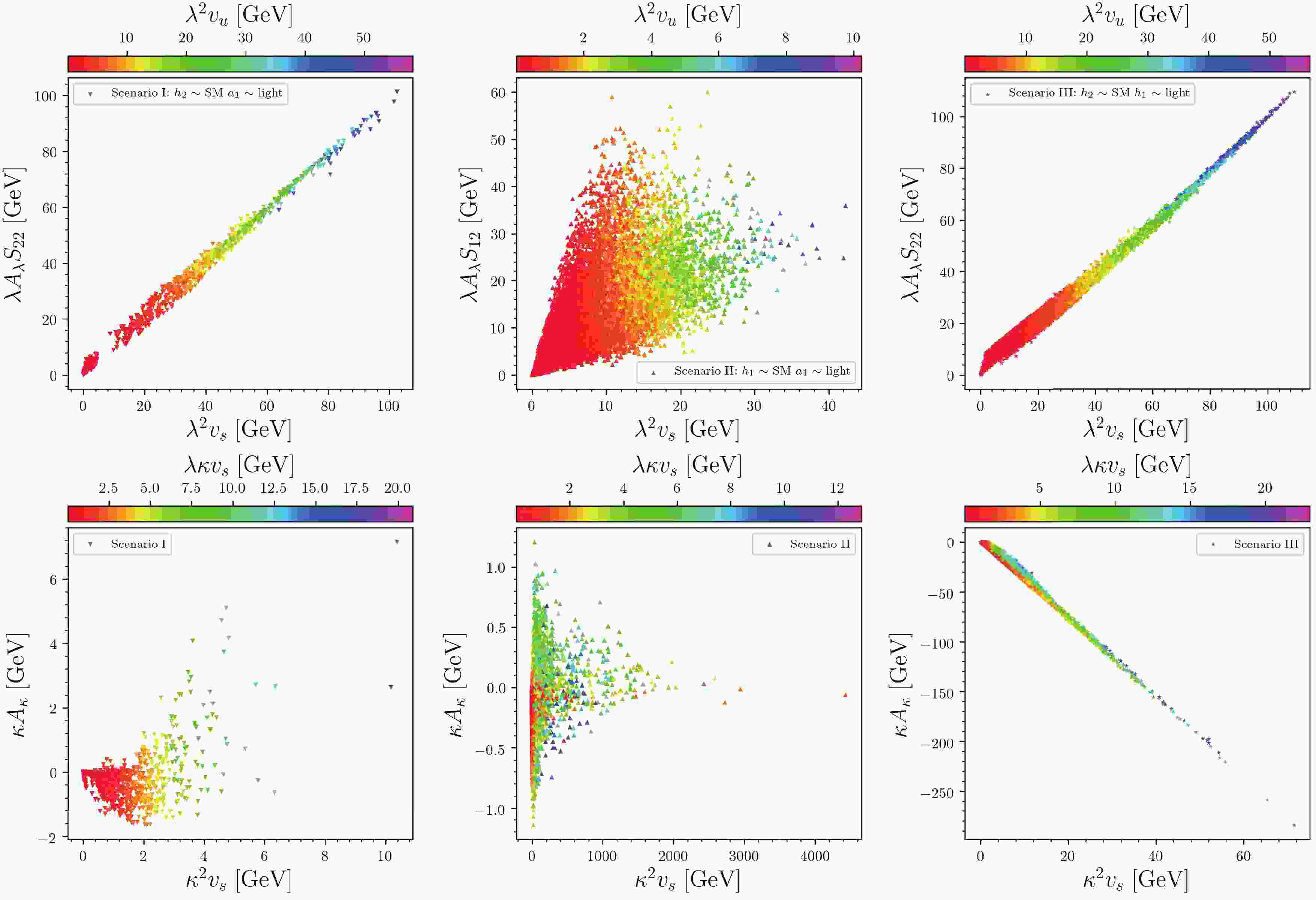
To study the different mechanisms of Higgs decay to light scalars in different scenarios, we recombine relevant parameters and show them in Fig. 1. From this figure, one can find the following:

Figure 1. (color online) Surviving samples for the three scenarios in the
$ \lambda A_\lambda S_{i2} $ versus$ \lambda^2 v_s $ (upper), where$ S_{22} $ (left and right) and$ S_{12} $ (middle) are the down-type-doublet component coefficient in the SM-like Higgs, and$ \kappa A_\kappa $ versus$ \kappa^2 v_s $ (lower) planes, respectively. Colors indicate$ \lambda^2 v_u $ (upper) and$ \lambda\kappa v_s $ (lower), respectively.• For Scenarios I and III,
$ \lambda A_{\lambda}S_{22} \!\approx\! \lambda^2v_s $ , where$ 0.03\!\lesssim\! S_{22}\!\lesssim\!0.07 $ is at the same order with$ 1/\tan\!\beta $ , for the mass scale of the CP-odd doublet scalar$ M_A \!\thicksim\! 2\mu_{\rm{eff}}/ \sin\!2\beta \!\thicksim\! A_{\lambda} \!\gg\! \kappa v_s $ , and$ \tan\!\beta\!\gg\!1 $ [33]. Thus, the SM-like Higgs is up-type-doublet dominated.• For Scenario I,
$ \kappa A_{\kappa} $ ,$ k^2v_s $ , and$ \lambda\kappa v_s $ are at the same level of a few GeV; however, for Scenario II,$ \kappa^2 v_s $ can be as large as a few TeV for small$ \lambda $ and large$ \kappa $ .• Especially, for Scenario III,
$ \kappa A_{\kappa} \!\approx\! -4\kappa^2 v_s $ , or$ A_\kappa \!\approx\! -4\kappa v_s $ .According to the large data of the
$ 125 \; {{\rm{GeV}}} $ Higgs and current null results searching for non-SM Higgs, the$ 125 \; {{\rm{GeV}}} $ Higgs should be doublet dominated, and the light scalar should be singlet dominated. In our cases, we found that, in the CP-even sector, the mixing between singlet and up-type doublet$ \eta_{us} $ , the mixing between down-type doublet and up-type doublet$ \eta_{ud} $ , and the mixing between singlet and down-type doublet$ \eta_{ds} $ are, respectively, roughly equal to$ \begin{aligned}[b] \eta_{us} \approx &\frac{2\lambda v \mu_{\rm{eff}} \left[ 1-\left(\dfrac{M_A}{2\mu/\sin2\beta}\right)^2 -\dfrac{\kappa}{2\lambda}\sin2\beta\right]}{m_h^2-m_s^2} \,, \\ \eta_{ud} \approx & \frac{1}{\tan\beta} \,, \\ \eta_{ds} \approx & -\frac{\eta_{us}}{\tan\beta} \,, \end{aligned} $

(17) where
$ m_h $ and$ m_s $ are masses of the SM-like Higgs and the singlet-dominated CP-even scalar, respectively, and$ |\eta_{ds}| \ll |\eta_{us}|, |\eta_{ud}| \ll 1 \,. $

(18) And in the CP-odd sector, the mixing between singlet and down-type doublet
$ \eta'_{ds} $ , the mixing between down-type doublet and up-type doublet$ \eta'_{ud} $ , and the mixing between singlet and up-type doublet$ \eta'_{us} $ are, respectively, roughly equal to$ \begin{aligned}[b] \eta'_{ds} \approx &\dfrac{\lambda v \dfrac{M_A^2}{2\mu_{\rm{eff}}/\sin2\beta} -3 \kappa v \mu_{\rm{eff}}}{m^2_{a_2}-m^2_{a_1}} \approx \dfrac{\lambda v}{\mu_{\rm{eff}} \tan\beta} \,, \\ \eta'_{ud} \approx & \frac{1}{\tan\beta} \,, \\ \eta'_{us} \approx & -\frac{\eta'_{ds}}{\tan\beta} \,, \end{aligned} $

(19) where
$ |\eta'_{us}| \ll |\eta'_{ds}|, |\eta'_{ud}| \ll 1 \,. $

(20) Specifically, in Scenario I,
$ S_{23} = \eta_{us}\,,\; \; \; S_{22} = \eta_{ud}\,,\; \; \; P_{11} = \eta'_{us}\,,\; \; \; P_{12} = \eta'_{ds}\,; \; \; \; $

(21) in Scenario II,
$ S_{13} = \eta_{us}\,,\; \; \; S_{12} = \eta_{ud}\,,\; \; \; P_{11} = \eta'_{us}\,,\; \; \; P_{12} = \eta'_{ds}\,; \; \; \; $

(22) in Scenario III,
$S_{23} = \eta_{us}\,,\; \; \; S_{22} = \eta_{ud}\,,\; \; \; S_{11} = -\eta_{us}\,,\; \; \; S_{12} = \eta_{ds}\,. \; \; \; $

(23) In Fig. 2, we show how small they can be and their relative scale. From this figure, we can see the following for the three scenarios.
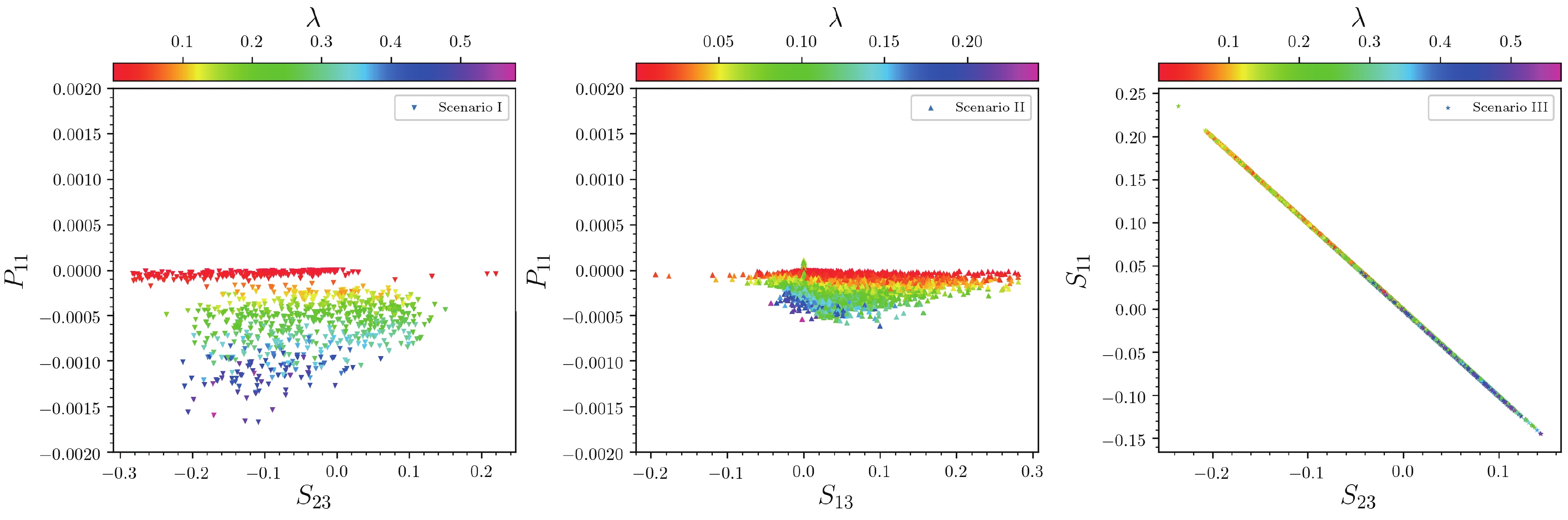
Figure 2. (color online) Surviving samples for the three scenarios in the
$ P_{11} $ versus$ S_{23} $ (left),$ P_{11} $ versus$ S_{13} $ (middle), and$ S_{11} $ versus$ S_{23} $ (right) planes, respectively, where$ S_{23} $ (left and right) and$ S_{13} $ (middle) are the singlet component in the SM-like Higgs, and$ P_{11} $ (left and middle) and$ S_{11} $ (right) are the up-type-doublet components of the light scalar, respectively. Colors indicate the parameter$ \lambda $ .• Scenario I: The up-type-doublet component of the light scalar,
$ -\!0.0015 \!\lesssim\! P_{11} \!<\!0 $ , is proportional to the parameter$ \lambda $ ; thus, the total doublet component of the light scalar is$ P_{1D}\!\equiv\! \sqrt{P_{11}^2+P_{12}^2}\!\thickapprox\! P_{11}\tan\beta \!\lesssim\!0.04 $ , while the singlet component of the SM-like Higgs is$ |S_{23}|\!\lesssim\!0.3 $ .• Scenario II: The up-type-doublet component of the light scalar,
$ -\!0.0006 \!\lesssim\!P_{11}\!<\!0 $ , is proportional to the parameter$ \lambda $ ; thus, the total doublet component of the light scalar is$ 0<P_{1D}\!\lesssim\!0.013 $ , while the singlet component in the SM-like Higgs is$ |S_{13}|\!\lesssim\!0.3 $ .• Scenario III: The up-type-doublet component of the light scalar and the singlet component of the SM-like Higgs are anticorrelated, i.e.,
$ S_{11}\!\thickapprox\!-S_{23} $ , and their range is$ -0.15\!\lesssim\! S_{11}\!\lesssim\! 0.2 $ , with the sign related to the parameter$ \lambda $ . This also means that the mixing in the CP-even scalar sector is mainly between the singlet and the up-type doublet, and we found that$ 0.03\!\lesssim\!S_{22}\!\lesssim0.07 $ and$ S_{12}\!\lesssim\!0.03 $ . Thus, the SM-like Higgs is up-type doublet dominated, which is applicable in all three scenarios, with$ S_{21}\!\approx\! 1 $ in Scenario I and III and$ S_{11}\!\approx\!1 $ in Scenario II.Considering the values of and correlations among parameters and component coefficients, the couplings between the SM-like Higgs and a pair of light scalars can be simplified as
$ C_{h_2a_1a_1} \!\simeq \! \sqrt{2}\lambda^2v_u+\sqrt{2}\lambda A_{\lambda}P_{11}\tan\!\beta\,, $

(24) $ C_{h_1a_1a_1}\! \simeq\! \sqrt{2}\lambda^2v_u\!+\!\!\sqrt{2}\lambda A_{\lambda}P_{11}\tan\!\beta \!+\!2\!\sqrt{2}\kappa^2v_s S_{13} \,, \!\!\!\!\! $

(25) $ \begin{aligned}[b] C_{h_2h_1h_1} \simeq & \sqrt{2}\lambda^2v_u-\sqrt{2}\lambda A_{\lambda}S_{12} +\sqrt{2}\lambda^2v_s S_{11} \\ &+2\sqrt{2}\kappa^2 v_sS_{23} +\frac{3g^2}{\sqrt{2}}v_u S_{11}S_{11} \\ &-2\sqrt{2}\lambda\kappa v_s S_{12} \,. \end{aligned} $

(26) In Fig. 3, we show the exotic branching ratio
$ Br(h\!\to\!ss) $ including one-loop correction correlated with the mass of the light scalar and the coupling between the SM-like Higgs and a pair of the light scalars at tree level. Since the 125 GeV Higgs is constrained to be very SM-like, its decay widths and branching ratios to SM particles cannot vary much, which leads indirectly to strong upper limits on exotic branching ratios of the SM-like Higgs [3-5]①. Thus, combined with Eq. (9), it is natural that the branching ratios to light scalars are proportional to the square of the tri-scalar couplings. The significant deviations for the negative-coupling samples in Scenario III are because of the one-loop correction of the stop loops,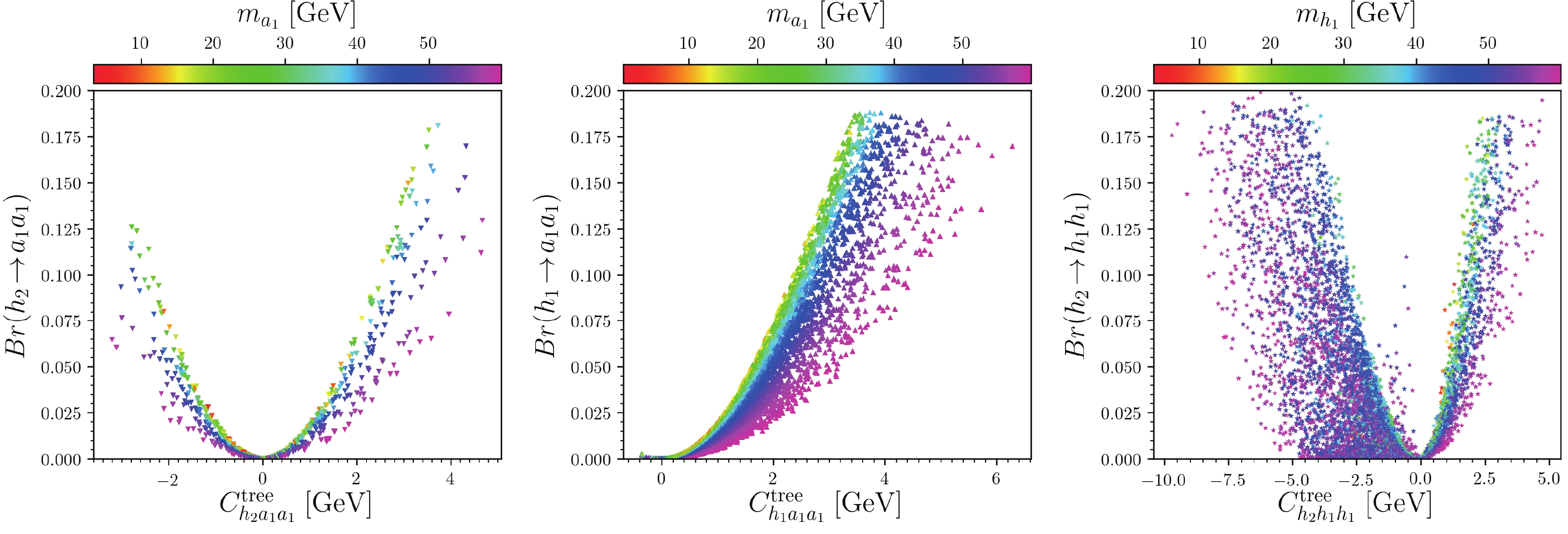
Figure 3. (color online) Surviving samples for the three scenarios in the exotic branching ratio
$ Br(h\!\to\!ss) $ versus the tri-scalar coupling$ C_{hss}^{\rm{tree}} $ at tree level planes, respectively, with colors indicating the mass of light Higgs$ m_s $ , where$ h $ denotes the SM-like Higgs$ h_2 $ (left and right) and$ h_1 $ (middle), and$ s $ denotes the light scalar$ a_1 $ (left and middle) and$ h_1 $ (right).$ \Delta C_{h_2h_1h_1} \simeq S_{21} S_{11}^2 \frac{3\sqrt{2}m_t^4}{16\pi^2 v_u^3} \ln \left( \frac{m_{\tilde{t}_1}m_{\tilde{t}_2}}{m_t^2}\right), $

(27) which can be as large as
$ 5 \; {{\rm{GeV}}} $ , whereas for Scenario I and II, they are$ \Delta C_{h_2a_1a_1} \simeq S_{21} P_{11}^2 \frac{3\sqrt{2}m_t^4}{16\pi^2 v_u^3} \ln \left( \frac{m_{\tilde{t}_1}m_{\tilde{t}_2}}{m_t^2}\right), $

(28) $ \Delta C_{h_1a_1a_1} \simeq S_{11} P_{11}^2 \frac{3\sqrt{2}m_t^4}{16\pi^2 v_u^3} \ln \left( \frac{m_{\tilde{t}_1}m_{\tilde{t}_2}}{m_t^2}\right). $

(29) Since
$ P_{11}\!\ll\! S_{11} $ , as seen from Fig. 2, the loop correction in Scenarios I and II is much smaller than that in Scenario III. In the following figures and discussions, we consider the coupling$ C_{hss} $ to include the one-loop correction$ \Delta C_{hss} $ , unless otherwise specified. -
At the LHC, the SM-like Higgs can first be produced in gluon fusion (ggF), vector boson fusion (VBF), associated with vector boson (Wh, Zh), or associated with
$ t\bar{t} $ processes, where the cross section in the ggF process is much larger than that of others. Then, the SM-like Higgs can decay to a pair of light scalars, and each scalar can then decay to a pair of fermions, gluons, or photons. The ATLAS and CMS collaborations have searched for these exotic decay modes in the final states of$ b\bar{b}\tau^+\tau^- $ [11],$ b\bar{b}\mu^+\mu^- $ [12,13],$ \mu^+\mu^-\tau^+\tau^- $ [14-16],$ 4\tau $ [16,17],$ 4\mu $ [18-20],$ 4b $ [21],$ \gamma\gamma gg $ [22],$ 4\gamma $ [23], etc. These results are included in the constraints we considered.As we checked, the main decay mode of the light scalar is usually to
$ b\bar{b} $ when$ m_s\gtrsim 2m_b $ . However, the color backgrounds at the LHC are very large; thus, a subleading Zh production process is used in detecting$ h\!\!\to\!\! 2s \!\!\to\!\! 4b $ , and VBF is used for$ h\!\!\to\!\! 2s \!\!\to\!\! \gamma\gamma gg $ . For the other decay mode, the main production process ggF can be used. Considering the cross sections of production and branching ratios of decay, as well as the detection precisions, we found that the detections in$ 4b $ ,$ 2b2\tau $ , and$ 2\tau 2\mu $ channels are important for the scNMSSM. The signal rates are$ \mu_{\rm{Zh}} \!\times\! Br(h\!\to\! ss \!\to\! 4b) $ ,$ \mu_{\rm{ggF}} \!\times\! Br(h\!\to\! ss \!\to\! 2b2\tau) $ , and$ \mu_{\rm{ggF}} \!\times\! Br(h\!\to\! ss \!\to\! 2\tau2\mu) $ , respectively, where$ \mu_{\rm{ggF}} $ and$ \mu_{\rm{Zh}} $ are the ggF and Zh production rates normalized to their SM value, respectively [3-5]②.For detections of the exotic decay at the HL-LHC, we use the simulation results of 95% exclusion limit in Refs. [24,33]. Suppose, with an integrated luminosity of
$ L_0 $ , the 95% exclusion limit for branching ratio in some channel is$ Br_0 $ in the simulation result; then, for a sample in the model, if the signal rate is$ \mu_i\!\times\! Br $ ($ i $ denotes the production channel), the signal significance with integrated luminosity of$ L $ will be$ ss = 2 \;\frac{\mu_i\!\times\! Br}{Br_0} \sqrt{\frac{L}{L_0}}, $

(30) and the integrated luminosity needed to exclude the sample in the channel at 95% confidence level (with
$ ss = 2 $ ) will be$ L_{\rm{e}} = L_0 \left(\frac{Br_0}{\mu_i\!\times\! Br}\right)^2, $

(31) and the integrated luminosity needed to discover the sample in the channel (with
$ ss = 5 $ ) will be$ L_{\rm{d}} = L_0 \left(\frac{5}{2}\right)^2 \left(\frac{Br_0}{\mu_i\!\times\! Br}\right)^2. $

(32) In Figs. 4, 5, and 6, we show the signal rates for the surviving samples in the three scenarios and the 95% exclusion bounds [24,33] in the
$ 4b $ ,$ 2b2\tau $ , and$ 2\tau2\mu $ channels, respectively. From these figures, one can see the following: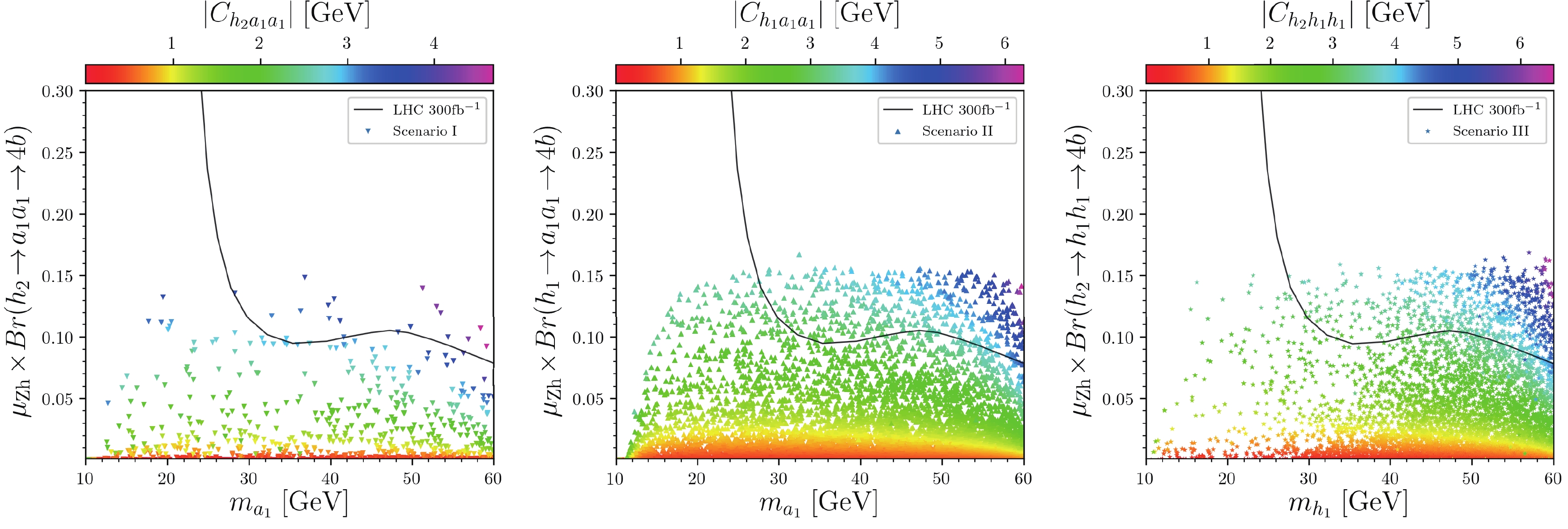
Figure 4. (color online) Surviving samples for the three scenarios in the signal rate
$ \mu_{\rm{Zh}} \!\times\! Br(h\!\to\! ss\!\to\! 4b) $ versus the mass of light Higgs$ m_s $ planes, respectively, with colors indicating the tri-scalar coupling$ C_{hss} $ including one-loop correction, where$ h $ denotes the SM-like Higgs$ h_2 $ (left and right) and$ h_1 $ (middle), and$ s $ denotes the light scalar$ a_1 $ (left and middle) and$ h_1 $ (right). The solid curves indicate the simulation results of the 95% exclusion limit in the corresponding channel at the HL-LHC with$ 300 {\; {\rm{fb}}}^{-1} $ [33].
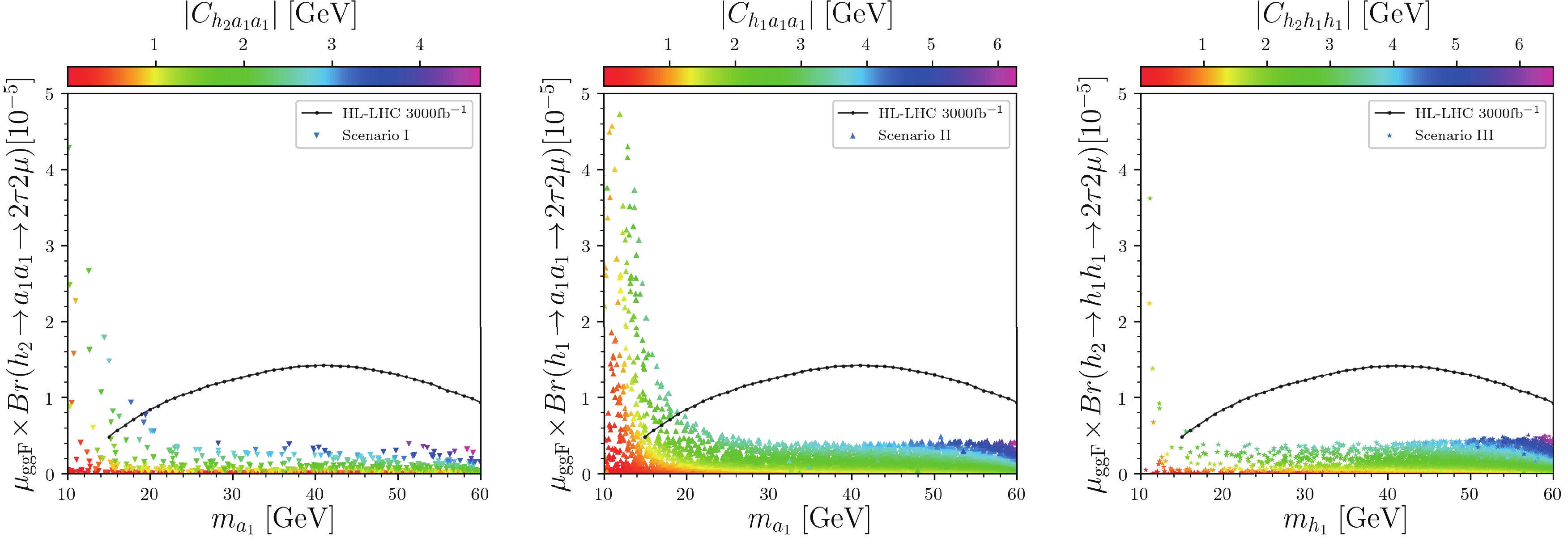
• With a light scalar heavier than
$ 30 \; {{\rm{GeV}}} $ , the easiest way to discover the exotic decay is via the$ 4b $ channel, and the minimal integrated luminosity needed to discover the decay in this channel can be$ 650 {\; {\rm{fb}}}^{-1} $ for Scenario II.• With a light scalar lighter than
$ 20 \; {{\rm{GeV}}} $ , the$ 2\tau2\mu $ channel can be important, especially for samples in Scenario II, and the minimal integrated luminosity needed to discover the decay in this channel can be$ 1000 {\; {\rm{fb}}}^{-1} $ .• With a light scalar heavier than
$ 2m_b $ , it is possible to discover the decay in the$ 2b2\tau $ channel, and the minimal integrated luminosity needed to discover the decay in this channel can be$ 1500 {\; {\rm{fb}}}^{-1} $ for Scenario II. -
In future lepton colliders, such as CEPC, FCC-ee, and International Linear Collider (ILC), the main production process of the SM-like Higgs is Zh, and the color backgrounds are minimal; thus, these lepton colliders are powerful in detecting the exotic decay. There have been simulation results in many channels, such as
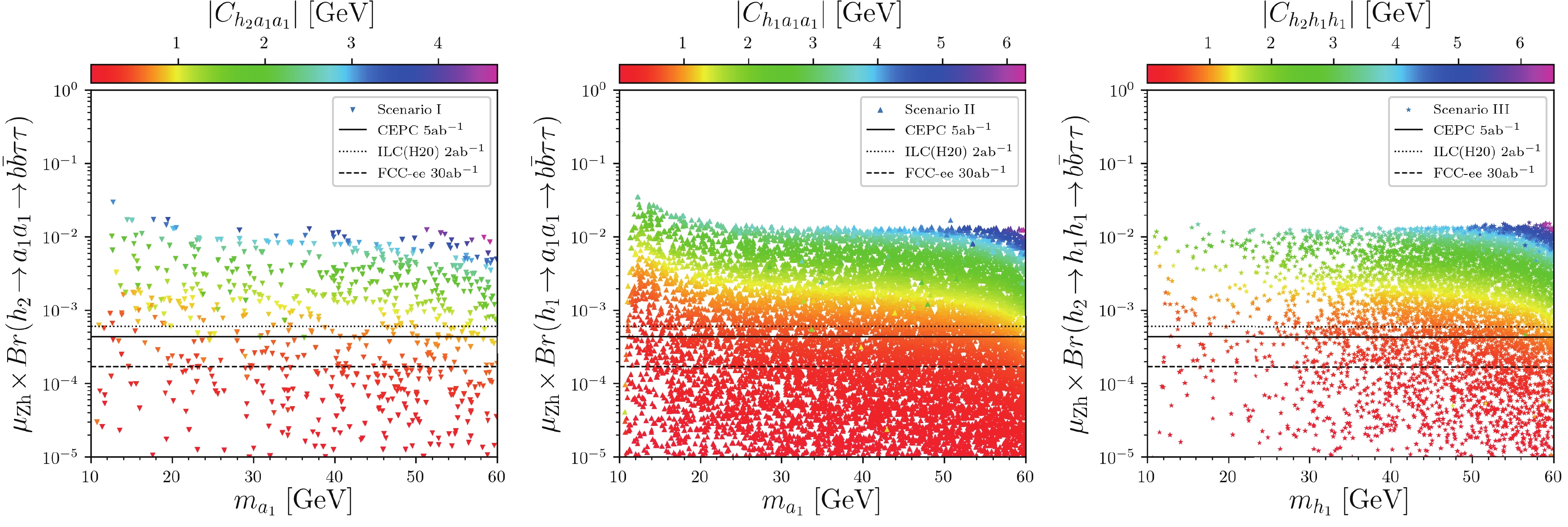
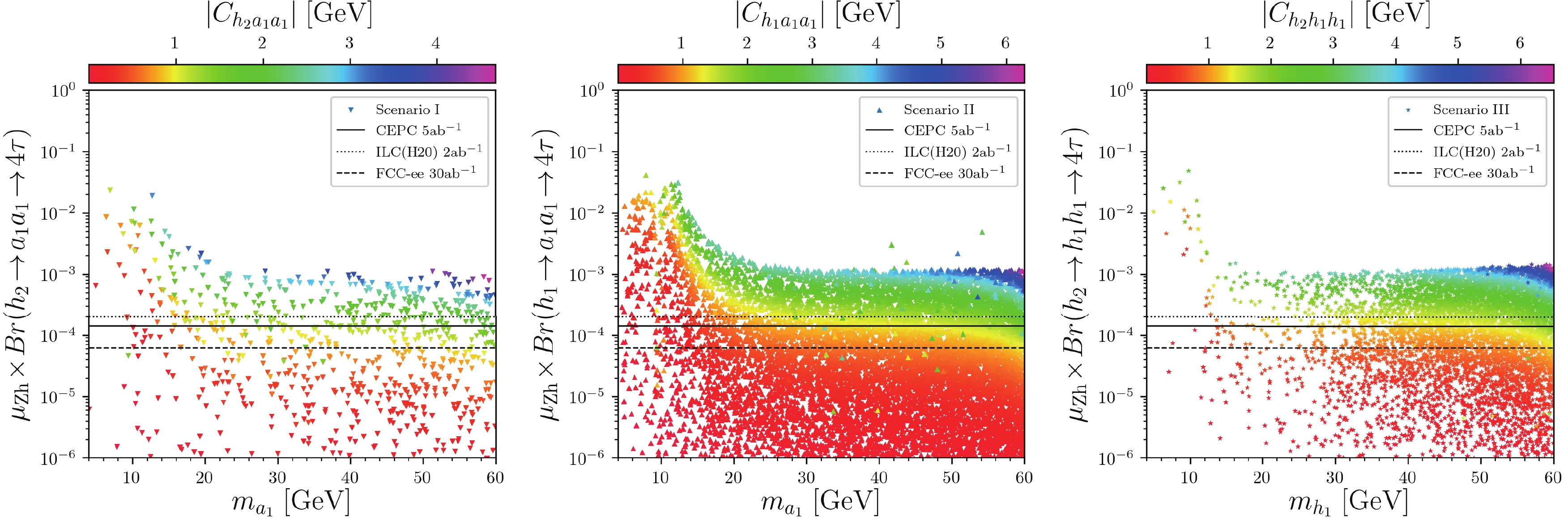
$ 4b $ ,$ 4j $ ,$ 2b2\tau $ , and$ 4\tau $ [26]. With the same method as in the last subsection, one can perform similar analyses.In Figs. 7, 8, 9, and 10, we show the signal rates for surviving samples in the three scenarios and the 95% exclusion bounds (following the simulation results in Ref. [26]) at the CEPC, FCC-ee, and ILC, and in the
$ 4b $ ,$ 4j $ ,$ 2b2\tau $ , and$ 4\tau $ channels, respectively. In these processes, the backgrounds are mainly from SM Higgs decays to four light particles through SM gauge bosons. From these figures, one can see the following: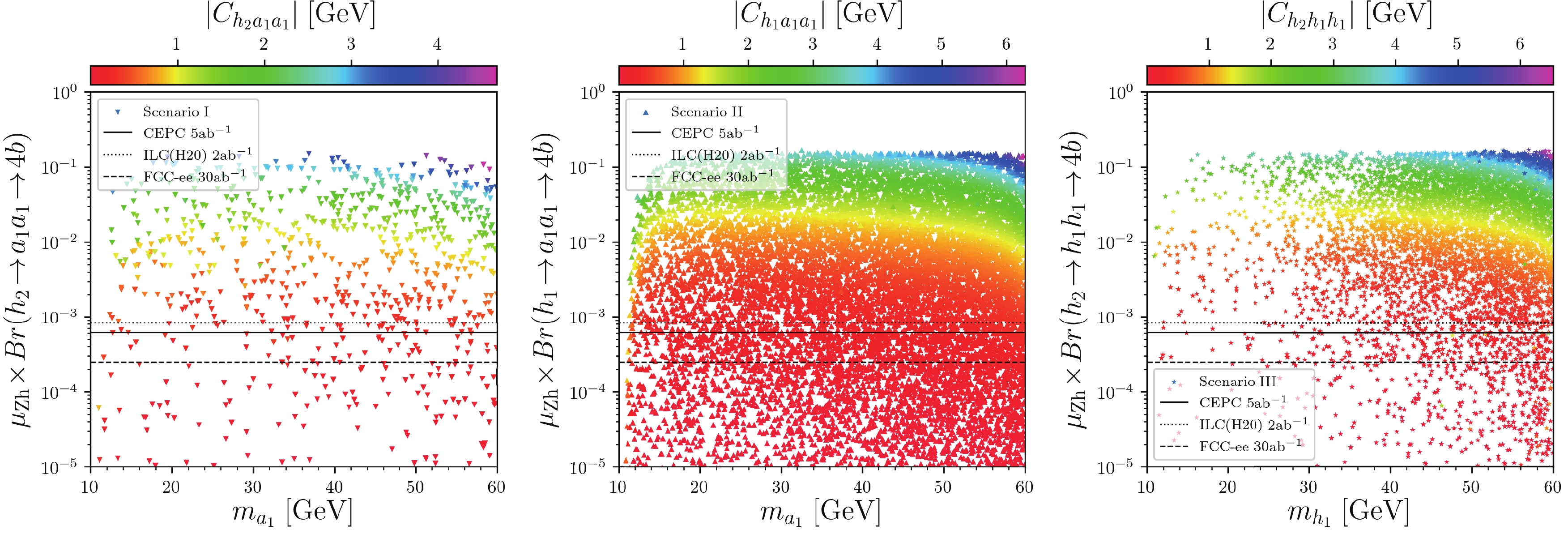
Figure 7. (color online) Surviving samples for the three scenarios in the signal rate
$ \mu_{\rm{Zh}} \!\times\! Br(h\!\to\! ss\!\to\! 4b) $ versus the mass of light Higgs$ m_s $ planes, respectively, with colors indicating the tri-scalar coupling$ C_{hss} $ including one-loop correction, where$ h $ denotes the SM-like Higgs$ h_2 $ (left and right) and$ h_1 $ (middle), and$ s $ denotes the light scalar$ a_1 $ (left and middle) and$ h_1 $ (right). The solid, dashed, and dotted lines are the 95% exclusion bounds from simulations in the corresponding channel at the CEPC with$ 5\,{\rm{ab}}^{-1} $ , FCC-ee with$ 30\,{\rm{ab}}^{-1} $ , and ILC with$ 2\,{\rm{ab}}^{-1} $ , respectively [26].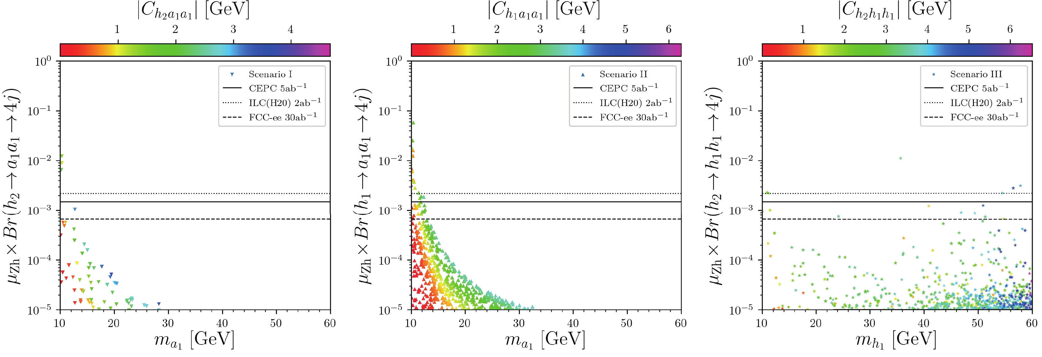
• As in Fig. 7, when the light scalar is heavier than approximately
$ 15 \; {{\rm{GeV}}} $ and the tri-scalar coupling is large enough, the branching ratio for the$ 4b $ channel is significant. The minimal integrated luminosity needed to discover the decay in this channel can be$ 0.31 {\; {\rm{fb}}}^{-1} $ for Scenarios II and III at the ILC.• As in Fig. 8, for Scenarios I and II, the exotic Higgs decay can be expected to be observed in the
$ 4j $ channel when its mass is lighter than$ 11 \; {{\rm{GeV}}} $ , whereas for Scenario III, the light scalar available at the CEPC can be as heavy as$ 40 \; {{\rm{GeV}}} $ . The minimal integrated luminosity needed to discover the exotic decay in this channel can be$ 18 {\; {\rm{fb}}}^{-1} $ for Scenario II at the ILC.• As in Figs. 9 and 10, the signal rates in
$ 2b2\tau $ and$ 4\tau $ channel show similar trends. The branching ratios are small before the light scalar reaches the mass threshold, and the maximum values of branching ratios occur around$ m_s = 12 \; {{\rm{GeV}}} $ ; the minimal integrated luminosity needed to discover the decay in the$ 2b2\tau $ channel is$ 3.6 {\; {\rm{fb}}}^{-1} $ for Scenario II at the ILC, and that in the$ 4\tau $ channel is$ 0.22 {\; {\rm{fb}}}^{-1} $ for Scenario III at the ILC. -
In this work, we have discussed the exotic Higgs decay to a pair of light scalars in the scNMSSM, or the NMSSM with NUHM. First, we performed a general scan over the nine-dimension parameter space of the scNMSSM, considering the theoretical constraints of vacuum stability and Landau pole as well as experimental constraints of Higgs data, non-SM Higgs searches, muon g-2, sparticle searches, relic density and direct searches for dark matter, etc. Then, we found three scenarios with a light scalar of
$ 10\sim 60 \; {{\rm{GeV}}} $ : (i) the light scalar is CP-odd, and the SM-like Higgs is$ h_2 $ ; (ii) the light scalar is CP-odd, and the SM-like Higgs is$ h_1 $ ; and (iii) the light scalar is CP-even, and the SM-like Higgs is$ h_2 $ . For the three scenarios, we check the parameter regions that lead to the scenarios, the mixing levels of the doublets and singlets, the tri-scalar coupling between the SM-like Higgs and a pair of light scalars, the branching ratio of Higgs decay to the light scalars, and the detections at the hadron colliders and future lepton colliders.In this work, we compare the three scenarios, checking the interesting parameter regions that lead to the scenarios, the mixing levels of the doublets and singlets, the tri-scalar coupling between the SM-like Higgs and a pair of light scalars, the branching ratio of Higgs decay to the light scalars, and the detections at the hadron colliders and future lepton colliders.
Finally, we draw the following conclusions regarding a light scalar and the exotic Higgs decay to a pair of it in the scNMSSM:
• There are different interesting mechanisms in the three scenarios to tune parameters to obtain the small tri-scalar couplings.
• The singlet components of the SM-like Higgs in the three scenarios are at the same level of
$ \lesssim0.3 $ and are roughly one order of magnitude larger than the doublet component of the light scalar in Scenario I and II.• The couplings between the SM-like Higgs and a pair of light scalars at tree level are
$ -3\sim 5 $ ,$ -1\sim 6 $ , and$ -10\sim 5 $ GeV for Scenario I, II, and III, respectively.• The stop-loop correction to the tri-scalar coupling in Scenario III can be a few GeV, much larger than those in Scenarios I and II.
• The most effective way to discover the exotic decay at the future lepton collider is via the
$ 4\tau $ channel, while that at the HL-LHC is via the$ 4b $ channel for a light scalar heavier than 30 GeV and via$ 2b2\tau $ or$ 2\tau2\mu $ channel for a lighter scalar.The details of the minimal integrated luminosity needed to discover the exotic Higgs decay at the HL-LHC, CEPC, FCC-ee, and ILC are summarized in Table 2, and the tuning mechanisms in the three scenarios to obtain the small tri-scalar coupling can be seen from Figs. 1,2 and Eqs. (17)-(26).
Decay Mode Futrue colliders HL-LHC CEPC FCC-ee ILC ( $ b\bar{b} $ )(

$ b\bar{b} $ )

$ 650 {\; {\rm{fb}}}^{-1} $ (@II)

$ 0.42 {\; {\rm{fb}}}^{-1} $ (@III)

$ 0.41 {\; {\rm{fb}}}^{-1} $ (@III)

$ 0.31 {\; {\rm{fb}}}^{-1} $ (@II)

( $ jj $ )(

$ jj $ )

− $ 21 {\; {\rm{fb}}}^{-1} $ (@II)

$ 18 {\; {\rm{fb}}}^{-1} $ (@II)

$ 25 {\; {\rm{fb}}}^{-1} $ (@II)

( $ \tau^+\tau^- $ )(

$ \tau^+\tau^- $ )

− $ 0.26 {\; {\rm{fb}}}^{-1} $ (@III)

$ 0.22 {\; {\rm{fb}}}^{-1} $ (@III)

$ 0.31 {\; {\rm{fb}}}^{-1} $ (@III)

( $ b\bar{b} $ )(

$ \tau^+\tau^- $ )

$ 1500 {\; {\rm{fb}}}^{-1} $ (@II)

$ 4.6 {\; {\rm{fb}}}^{-1} $ (@II)

$ 3.6 {\; {\rm{fb}}}^{-1} $ (@II)

$ 4.4 {\; {\rm{fb}}}^{-1} $ (@II)

( $ \mu^+\mu^- $ )(

$ \tau^+\tau^- $ )

$ 1000 {\; {\rm{fb}}}^{-1} $ (@II)

− − − Table 2. The minimum integrated luminosity for discovering (at
$ 5\sigma $ level) the exotic Higgs decay at the future colliders, where "@I, II, III" indicates the three different scenarios.
Higgs decay to light (pseudo)scalars in the semi-constrained NMSSM
- Received Date: 2020-08-24
- Accepted Date: 2020-11-17
- Available Online: 2021-02-15
Abstract: The next-to minimal supersymmetric standard model (NMSSM) with non-universal Higgs masses, i.e., the semi-constrained NMSSM (scNMSSM), extends the minimal supersymmetric standard model (MSSM) by a singlet superfield and assumes universal conditions, except for the Higgs sector. It can not only maintain the simplicity and grace of the fully constrained MSSM and NMSSM and relieve the tension they have been facing since the discovery of the 125-GeV Higgs boson but also allow for an exotic phenomenon wherein the Higgs decay into a pair of light (


 DownLoad: