


 Abstract
 HTML
HTML Reference
 Related
 PDF
PDF


-
The oscillation pattern observed from the solar and atmospheric neutrinos has surprisingly revealed a small (but nonzero) mass for these particles [1]. From the theoretical point of view, the seesaw mechanism is the most popular approach for generating small masses for neutrinos [2-6].
The observation of galaxy rotational curves [7] and cluster collisions [8] as well as the precise measurements of the thermal anisotropy of the cosmic microwave background [9] suggest the existence of dark matter (DM) permeating our universe. Recent results from PLANCK satellite indicate that 26.7% of the energy content of the universe is in the form of non-luminous matter [9]. The most popular DM candidate is a weakly interactive massive particle (WIMP) [10, 11]. WIMPs can be any type of particle, as long as they fulfill a series of conditions, such as neutrality and stability (or sufficiently long lived), and have mass in the range of a few GeVs up to a few TeVs.
Cosmological inflation is considered the best theory for explaining homogeneity, flatness, and isotropy of the universe, as required by hot big bang [12-14]. Experiments in cosmology, such as WMAP7 and Planck2018 [9, 15], entered an era of precision that allowed us to probe scenarios that try to explain the primordial universe. Single-field slow-roll models of inflation coupled non-minimally to gravity seems to be an interesting scenario for inflation [16, 17], given that it connects inflation to particle physics at low energy scale [17].
Although the Standard Model (SM) of particle physics is a very successful theory, its framework does not accommodate any of the three issues discussed above. In other words, nonzero neutrino mass, dark matter, and inflation require extensions of the SM.
In this study, we show that the
$U(1)_{\rm B-L}$ (B-L) gauge model is capable of accomplishing all these three issues in a very attractive way by simply adding a scalar triplet to its canonical scalar sector [18-22] and resorting to an adequate$ Z_2 $ symmetry. Interestingly, we have that small neutrino masses are achieved through the type II seesaw mechanism, which is triggered by the spontaneous breaking of the B-L symmetry, while the dark matter content of the universe is composed by the lightest right-handed neutrino of the model. Furthermore, by allowing a non-minimal coupling between gravity and the triplet$ \Delta $ , we show that the model may perform inflation at high energy without loss of unitarity.This paper is organized as follows. In Section II, we describe the main properties of the B-L model. Section III is devoted to cosmological inflation. In Section IV, we describe our calculation of the dark matter candidate, and Section V contains our conclusions.
-
Baryon number (B) and lepton number (L) are accidental anomalous symmetries of the SM. However, it is well known that only some specific linear combinations of these symmetries can be free from anomalies [18, 23-25]. Among them, the most developed one is the B-L symmetry [18-21], which is involved in several physical scenarios, such as GUT [26], seesaw mechanism [2-5], and baryogenesis [27]. This symmetry gives rise to the simplest gauge extension of the SM, namely the B-L model, which is based on the gauge group
$SU(3)_C \times SU(2)_L \times U(1)_Y \times U(1)_{\rm B-L}$ . In this study, we considered an extension of the B-L model in which its canonical scalar sector is augmented by a scalar triplet. Thus, the particle content of the model involves the standard particles augmented by three right-handed neutrinos (RHNs),$ N_i \sim ({\bf 1}, {\bf 1},0,-1) \,\,, \,\, i = 1,2,3 $ , one scalar singlet,$ S\sim ({\bf 1}, {\bf 1}, 0,2) $ , and one scalar triplet,$ \Delta\equiv \left(\begin{array}{cc} \dfrac{\Delta^{+}}{\sqrt{2}} & \Delta^{++} \\ \Delta^{0} & \dfrac{-\Delta^{+}}{\sqrt{2}} \end{array} \right)\sim ({\bf 1}, {\bf 3}, 2, 2). $

(1) The values in parentheses refer to the transformation of the fields by the
$SU(3)_C \times SU(2)_L \times U(1)_Y \times U(1)_{\rm B-L}$ symmetry. To the best of our knowledge, there are few studies in which the triplet$ \Delta $ composes the scalar sector of the B-L model. For previous models, please refer to [28, 29]. Moreover, we imposed the model to be invariant by a$ Z_2 $ discrete symmetry with the RHNs transforming as$ N_i \rightarrow -N_i $ , while the rest of the particle content of the model transforms trivially by$ Z_2 $ .With these features, the Yukawa interactions of interest are composed by the terms
$ {\cal L}_{\rm B-L} \supset Y_\nu\overline{f^C}i\sigma^2 \Delta f + \frac{1}{2}Y_N\overline{N^c} N S + {\rm h.c.}, $

(2) where
$ f = (\nu \,\,\,\,e)_L^T \sim ({\bf 1}, {\bf 2},-1,-1) $ . Note that both neutrinos gain masses when$ \Delta^0 $ and S develop a nonzero vacuum expectation value ($ v_\Delta $ and$ v_S $ ). This yields the following expressions to the masses of these neutrinos$\begin{aligned}[b] m_\nu = \frac{Y_\nu v_\Delta}{\sqrt{2}}\quad m_{\nu_R} = \frac{Y_N v_S}{\sqrt{2}}. \end{aligned}$

(3) Small masses for
$ \nu $ 's require small$ v_\Delta $ . We will show that, on fixing$ v_h $ and$ v_S $ , we may obtain$ v_\Delta $ around eV scale for the type II seesaw mechanism [6, 30, 31]. To this end, we must develop the potential of the model, which is invariant by the B-L symmetry and involves the following terms$ \begin{aligned}[b] V(H,\Delta,S) = & \mu^2_h H^\dagger H + \lambda_h (H^\dagger H)^2 + \mu^2_s S^\dagger S + \lambda_s (S^\dagger S)^2 \\ & + \mu^2_\Delta Tr(\Delta^\dagger \Delta) + \lambda_\Delta Tr[(\Delta^\dagger \Delta)^2] +\lambda^\prime_\Delta Tr[(\Delta^\dagger \Delta)]^2 \\ & + \lambda_1 S^\dagger SH^\dagger H + \lambda_2 H^\dagger\Delta \Delta^\dagger H + \lambda_3 Tr(\Delta^\dagger \Delta)H^\dagger H \\ & + \lambda_4 S^\dagger STr(\Delta^\dagger \Delta) + (k H^Ti\sigma^2\Delta^\dagger HS + {\rm h.c.}). \end{aligned} $

(4) where
$ H = (h^+ \,\,\,h^0)^T \sim ({\bf 1}, {\bf 2}, 1,0) $ is the standard Higgs doublet.At this point, note that the presence of
$ v_\Delta $ modifies the masses of the standard gauge bosons$ W^{\pm} $ and$ Z^0 $ . Consequently, it softly modifies the$ \rho $ -parameter as follows:$\rho = \left({1+\dfrac{2v^2_\Delta}{v^2_h}}\right)\bigg/\left({1+\dfrac{4v^2_\Delta}{v^2_h}}\right)$ . The current electroweak precision data provide$ \rho = 1.00037 \pm$ 0.00023 [1]. This implies the following upper bound$ v_\Delta < 2.5 $ GeV.Let us obtain the set of minimum conditions that guarantees that such a potential develops to a minimum. Then, we assume that all neutral scalars develop vevs different from zero and shift the neutral scalar fields in the conventional way
$ S,h^0,\Delta^0\rightarrow \frac{1}{\sqrt{2}}(v_{S,h,\Delta}+R_{S,h,\Delta}+{\rm i}I_{S,h,\Delta}), $

(5) which is substituted in the potential above. As a result, we obtain the following set of minimum condition equations:
$ \begin{aligned}[b] & v_S\left(\mu^2_S + \frac{\lambda_1}{2}v^2_h + \frac{\lambda_4}{2}v^2_\Delta + \lambda_s v^2_S\right) -\frac{k}{2}v^2_h v_\Delta = 0, \\ & v_h \left(\mu^2_h + \frac{\lambda_1}{2}v^2_S + \frac{\lambda_2}{2}v^2_\Delta + \frac{\lambda_3}{2}v^2_\Delta + \lambda_h v^2_h - k v_\Delta v_S\right) = 0, \\ & v_\Delta \left(\mu^2_\Delta + \frac{\lambda_2}{2}v^2_h + \frac{\lambda_3}{2}v^2_h + \frac{\lambda_4}{2}v^2_S + (\lambda_\Delta + \lambda^{\prime}_\Delta) v^2_\Delta\right) -\frac{k}{2}v^2_h v_S = 0. \end{aligned} $

(6) For the study of vacuum stability and bound from these conditions that guarantee that the potential is stable and has a global minimum, please refer to Refs. [32-34].
Note that, on considering
$ \mu_\Delta >> (v_h, \,\,v_S,\,\,v_\Delta $ ), the third relation in Eq. (6) provides$ v_\Delta \approx \frac{k}{2}\frac{v^2_h v_S}{\mu^2_\Delta}. $

(7) Note that the role of the type II seesaw mechanism is to provide small vevs. In the canonical type II seesaw case, where
$ v_\Delta = \dfrac{v^2_h}{M} $ , with M being the scale of energy that characterizes the explicit violation of the lepton number, the standard vev ($ v_h = 247 $ GeV) requires$ M = 10^{14} $ GeV to have$ v_\Delta $ around eV scale [6, 30, 31].The scenario proposed and developed here is completely different from the canonical case, because we assume that the lepton number is violated spontaneously at TeV scale. Consequently, the relation among
$ v_\Delta $ and the other energy scales of the model is given in Eq. (7). In this case, when assuming that$ v_S $ belongs to the TeV scale; then,$ v_\Delta $ around eV scale requires$ \mu_\Delta \sim 10^9 $ GeV. Although this energy scale is much smaller than$ 10^{14} $ GeV, it is still high enough to be probed at current colliders. In other words, the scalars that compose the triplet$ \Delta $ are still heavy enough to be probed at the LHC. This is discussed below.As we will see, both
$ v_\Delta $ and$ v_S $ contribute to the mass of$ Z^{\prime} $ associated to the B-L symmetry. As$ v_\Delta << v_S $ ,$ v_S $ contributes predominantly to the mass of$ Z^{\prime} $ , which has a stringent constraint according to the LEP experiment [35]$ \frac{m_{Z^{\prime}}}{g_{\rm B-L}} \gtrsim 6.9\; {\rm{TeV}}. $

(8) In summary, the set of vevs that compose our scenario takes values as follows:
$ v_h = 247 $ GeV,$ v_S \sim $ TeV, and$ v_\Delta \sim $ eV. Then, the value of the masses of the standard neutrinos that accommodate solar and atmospheric neutrino oscillations is a question of adequate choice for the values of the Yukawa couplings$ Y_\nu $ 's, as expressed in Eq. (3). Concerning right-handed neutrinos, they will develop mass at TeV scale. We advocate here that the lightest right-handed neutrinos may play the role of the dark matter of the universe. This is plausible because it is a neutral particle that is protected by the$ Z_2 $ discrete symmetry. Moreover, as the scalars that compose the triplet are heavy particles, we also checked in which circumstances the neutral component of the triplet$ \Delta $ may perform inflation. Before addressing these points, we discuss the spectrum of scalars for such a scenario. -
Before advancing in this paper, it is necessary to discuss the scalar sector of the model briefly. Let us first focus on the CP-even sector. In the basis
$ (R_S,R_h,R_\Delta) $ , we have the following mass matrix:$ M^2_R = \left(\begin{array}{ccc} \dfrac{k}{2}\dfrac{v_\Delta v^2_h}{v_s}+2\lambda_S v^2_s & -kv_h v_\Delta + \lambda_1 v_s v_h & -\dfrac{k}{2} v^2_h + \lambda_4 v_s v_\Delta\\ -kv_h v_\Delta + \lambda_1 v_s v_h & 2\lambda_h v^2_h & -k v_s v_h + (\lambda_2 + \lambda_3) v_h v_\Delta \\ -\dfrac{k}{2} v^2_h + \lambda_4 v_s v_\Delta & -k v_s v_h + (\lambda_2 + \lambda_3) v_h v_\Delta & \dfrac{k}{2}\dfrac{v_s v^2_h}{v_\Delta} + 2(\lambda_\Delta + \lambda^\prime_\Delta)v^2_\Delta \end{array} \right). $

(9) Note that, for values of the vevs indicated above, the scalar
$ R_\Delta $ becomes very heavy, with$m^2_\Delta \sim \dfrac{k}{2}\dfrac{v_S v^2_h}{v_\Delta}$ , which implies that it decouples from the other ones. The other two quadratic masses are$ \begin{aligned}[b] m^2_h \simeq & 2\lambda_h v^2_h -\frac{1}{2}\frac{\lambda_1^2}{\lambda_S}v^2_h, \\ m^2_H \simeq & 2\lambda_S v^2_S +\frac{1}{2}\frac{\lambda_1^2}{\lambda_S}v^2_h, \end{aligned} $

(10) where
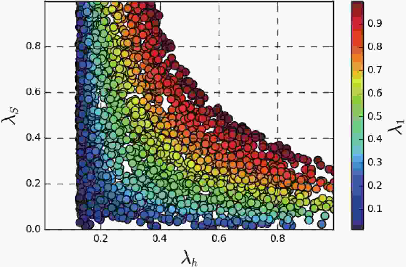
$ m_h $ denotes the standard Higgs boson, with the allowed parameter space shown in Fig. 1.
Figure 1. (color online) Possible values of the quartic couplings that yield 125 GeV Higgs mass.
The respective eigenvectors are
$ \begin{aligned}[b] h \simeq R_h-\frac{\lambda_1}{2\lambda_S}\frac{v_h}{v_s}R_S, \quad H \simeq R_S+\frac{\lambda_1}{2\lambda_S}\frac{v_h}{v_s}R_h. \end{aligned} $

(11) For the CP-odd scalars, we have the mass matrix in the basis
$ (I_S,I_h,I_\Delta) $ ,$ M^2_I = \left(\begin{array}{ccc} \dfrac{k}{2}\dfrac{v_\Delta v^2_h}{v_s} & kv_h v_\Delta & -\dfrac{k}{2} v^2_h \\ kv_h v_\Delta & 2k v_s v_\Delta & -k v_s v_h \\ -\dfrac{k}{2} v^2_h & -k v_s v_h & \dfrac{k}{2}\dfrac{v_s v^2_h}{v_\Delta} \end{array} \right). $

(12) The mass matrix in Eq. (12) can be diagonalized, providing one massive state
$ A^0 $ with mass$ m^2_A = \dfrac{k}{2}\left(\dfrac{v_\Delta v^2_h}{v_s} + \frac{v_s v^2_h}{v_\Delta} + 4v_s v_\Delta \right) $

(13) and two Goldstone bosons
$ G^1 $ and$ G^2 $ , absorbed as the longitudinal components of the Z and$ Z^{\prime} $ gauge bosons. The eigenvectors for the CP-odd scalars are$ \begin{aligned}[b] G^1 \simeq & I_S + \frac{v_\Delta}{v_s} I_\Delta, \\ G^2 \simeq & I_h + \frac{v_h}{2v_s} I_S, \\ A^0 \simeq & I_\Delta - \frac{2v_\Delta}{v_h} I_h. \end{aligned} $

(14) The charged scalars, given in the basis
$ (h^+,\Delta^+) $ , have the following mass matrix:$ M^2_+ = \left(\begin{array}{cc} k v_s v_\Delta - \dfrac{\lambda_2}{2}v^2_\Delta & \dfrac{\lambda _2}{2\sqrt{2}}v_h v_\Delta -\dfrac{k}{\sqrt{2}}v_s v_h \\ \dfrac{\lambda _2}{2\sqrt{2}}v_h v_\Delta -\dfrac{k}{\sqrt{2}}v_s v_h & \dfrac{k}{2} \dfrac{v_s v^2_h}{v_\Delta} - \dfrac{\lambda_2}{2}v^2_h \end{array}\right) . $

(15) Again, diagonalizing this matrix leads to two Goldstone bosons
$ G^\pm $ , responsible for the longitudinal parts of the$ W^\pm $ standard gauge bosons. The other two degrees of freedom give us the massive states$ H^\pm $ , with mass$ m^2_{H^\pm} = \left( \frac{v_\Delta}{2} + \frac{v^2_h}{4v_\Delta} \right)\left( 2k v_s - \lambda_2 v_\Delta \right). $

(16) The respective eigenvectors are
$ \begin{aligned}[b] G^\pm \simeq & h^{\pm} + \frac{\sqrt{2}v_\Delta}{v_h} \Delta^{\pm}, \\ H^{\pm} \simeq & \Delta^{\pm} - \frac{\sqrt{2}v_\Delta}{v_h}h^{\pm}. \end{aligned} $

(17) Finally, the mass of the doubly charged scalars
$ \Delta^{\pm \pm} $ are expressed as$ m^2_{\Delta^{\pm \pm}} = \frac{k v_s v^2_h v_\Delta - \lambda_2 v^2_h v^2_\Delta -2\lambda_\Delta v^4_\Delta}{2v^2_\Delta}. $

(18) Once symmetries are broken and the gauge bosons absorb the Goldstone bosons as longitudinal components, we have that the standard charged bosons present a contribution from the triplet vev,
$m^2_w = \dfrac{g^2}{4}\left(v^2_h + 2v^2_\Delta \right)$ , while the neutral gauge bosons become mixed with$ Z^{\prime} $ as follows:$ M^2_g = \left(\begin{array}{cc} \dfrac{g^2+g^{\prime 2}}{4}(v^2_h+4v_\Delta^2) & -g_{\rm B-L}\sqrt{g^2+g^{\prime 2}}v_\Delta^2 \\ -g_{\rm B-L}\sqrt{g^2+g^{\prime 2}}v_\Delta^2 & g^2_{\rm B-L}(2v_S+v_\Delta^2) \end{array} \right). $

(19) Keeping in mind the vev hierarchy discussed here (
$ v_S> v_h\gg v_\Delta $ ), the mixing between gauge bosons is very small; therefore, they decouple, resulting in the following masses:$ M^2_Z\approx \frac{(g^2+g^{\prime 2})( v^2_h + 4 v_\Delta^2)}{4}, \quad M^2_{Z^{\prime}}\approx 2g^2_{\rm B-L}\left(v^2_S+ \frac{v_\Delta^2}{2}\right). $

(20) Observe that we have a B-L model with new ingredients: scalars in the triplet and singlet forms and neutrinos with right-handed chiralities. Let us resume the role played by these new ingredients. The singlet S is responsible for the spontaneous breaking of the B-L symmetry and defines the mass of
$ Z^{\prime} $ . The triplet$ \Delta $ is responsible for the type II seesaw mechanism that generates small masses for the standard neutrinos. The right-handed neutrinos are responsible for the cancellation of anomalies. It would be interesting to find new roles for these components.We argue here, and check below, that the right-handed neutrinos may be the dark matter component of the universe, given that the
$ Z_2 $ symmetry protects them from decaying in lighter particles. In the last section, we assume that the lightest right-handed neutrino is the dark matter of the universe, calculate its abundance, and postulate possible ways of detecting it.We also argue here that once
$ \Delta^0 $ has mass around$ 10^9 $ GeV, it could be possible that it would come to be the inflaton and then drives inflation. We show in the next section that this is possible when we assume a non-minimal coupling of$ \Delta $ with gravity. -
The introduction of a non-minimal coupling between a scalar field and gravity to achieve successful inflation has become popular in recent years, although the original idea dates back to the eighties [16, 36, 37]. In particular, one may cite an extensive list of studies in which the standard Higgs field [17, 38-41] or a scalar singlet extension [42-44] assumed the role of inflaton. Although theoretically well motivated, such models may lead to a troublesome behavior in low-scale phenomenology. Concerning the case of Higgs Inflation, the measured Higgs mass pushes the non-minimal coupling to high values (
$ \xi \sim 10^4 $ ), causing unitarity issues at inflationary scale [45-48] (please refer to [49-51] for a different point of view). Similarly, the singlet scenario is also problematic. Although one could manage building a unitarily safe singlet inflation, this would produce a very light inflaton, placing in risk the reheating period of the universe [52].By contrast, the case in which a scalar triplet plays the role of inflaton is significantly different. Following the discussion in Section (IIB), note that the dominant terms in the scalar masses are independent of any parameter associated to inflation (
$ \lambda_\Delta, \lambda^\prime_\Delta,\xi $ ). In turn, this prevents the emergency of an excessively light inflaton, even for the smallest values of$ \lambda_\Delta $ and$ \lambda^\prime_\Delta $ . Such a configuration yields a unitarily safe inflationary model that does not place in risk the transition to the standard evolution of the universe. For previous studies on inflation based on$ \Delta $ , please refer to [52-54].For the sake of simplicity, we assume that
$ \Delta^0 $ provides the dominant coupling. This is equivalent to imposing that the effective masses of the Higgs doublet and the scalar singlet are greater than the Hubble scale as initial conditions of inflation. The analysis of inflationary scenarios with multiple fields coupled to gravity can be found in references [55, 56].The non-minimal coupling between the inflaton and gravity is defined in the Jordan frame, leading to the Lagrangian density
$ {\cal L} \supset \frac{1}{2} (\partial_\mu \Delta^0)^{\dagger}(\partial^\mu \Delta^0)-\frac{M_P^2R}{2}-\frac{1}{2}\xi {\Delta^0}^2 R -V(\Delta^0), $

(21) where R is the Ricci scalar, and
$ M_P = 2.435\times 10^{18} $ GeV is the reduced Planck mass. During inflation, the fourth order terms of the inflaton field dominate the scalar potential. Quantum effects are also supposed to play a key role in the inflationary dynamics. Here, we consider one-loop radiative corrections to the inflaton potential evaluated in the Jordan frame; these corrections are known as the Prescription II procedure [38, 39, 42, 43]. Such corrections encompass the standard and B-L gauge couplings g,$ g^{\prime} $ , and$g_{\rm B-L}$ , as well as the Yukawa couplings of the neutrinos. The result is a Coleman-Weinberg potential of the form [57, 58]$ V = \left( \frac{\lambda_{\Delta} + \lambda^{\prime}_{\Delta}}{4} + \frac{a}{32\pi^2}\ln{\frac{\Delta^0}{M_P}}\right){\Delta^0}^4 $

(22) and
$ a = 3\left(\frac{3}{2}g^4+{g^{\prime}}^4+{g_{B-L}}^4\right) +6g^2{g^{\prime}}^2 - \sum\limits_{i}Y^4_{\nu_i} + \sum\limits_{j} \lambda^2_j, $

(23) where
$ M_P $ is chosen for renormalization scale, the sum in i takes into account the three generations of neutrinos, and j runs for the scalar contributions ($ \lambda_{2} $ ,$ \lambda_{3} $ ,$ \lambda_{4} $ ,$ \lambda_{\Delta} $ , and$ \lambda^{\prime}_{\Delta} $ ).To calculate the parameters related to inflation, we must recover the canonical Einstein-Hilbert gravity. This process is called conformal transformation and can be understood through two steps. First, we re-scale the metric
$ \tilde{g}_{\alpha \beta} = \Omega^2 g_{\alpha \beta} $ . In doing so, the non-minimal coupling vanishes, but the inflaton acquires a non-canonical kinetic term. The process is finished by transforming the field into a form with canonical kinetic energy. Such transformation involves the relations [59, 60]$ \begin{aligned}[b] \tilde g_{\mu \nu}& = \Omega^2g_{\mu \nu}\,\,\,\,\,\,{\rm{where}} \,\,\,\,\, \Omega^2 = 1+\frac{\xi {\Delta^0}^2}{M^2_P}, \\ & \frac{{\rm d}\chi}{{\rm d}\Delta^0} = \sqrt{\frac{\Omega^2 +6\xi^2 {\Delta^0}^2/M_P^2}{\Omega^4}}. \end{aligned} $

(24) The Lagrangian in Einstein frame is given by
$ {\cal L} \supset -\frac{M^2_{P} \tilde R}{2}+\frac{1}{2} (\partial_\mu \chi)^{\dagger}(\partial^\mu \chi)-U(\chi)\,, $

(25) where
$U(\chi) = \dfrac{1}{\Omega^4}V\left(\Delta^0(\chi)\right)$ . There is some discussion about which frame is the physical one [61]; however, both frames agree in the regime of low energy.Inflation occurs whenever the field
$ \chi $ , or equivalently$ \Delta^0 $ , rolls slowly in a direction toward the minimum of the potential. The slow-roll parameters can be written as [62]$\epsilon = \frac{M^2_{P}}{2}\left(\frac{ U^{\prime}}{ U \chi^{\prime}}\right)^2, \quad \quad \eta = M^2_{P}\left( \frac{U^{\prime \prime}}{U \chi^{\prime}} - \frac{U^{\prime} \chi^{\prime \prime}} {U {\chi^{\prime}}^3}\right), $

(26) where
$ ^\prime $ indicate derivative with respect to$ \Delta^0 $ . Inflation starts when$ \epsilon,\eta \ll 1 $ and stops when$ \epsilon,\eta = 1 $ . In the slow-roll regime, we can write the spectral index and the tensor-to-scalar ratio as [63]$ n_S = 1-6\epsilon+2\eta, \quad \quad r = 16\epsilon. $

(27) Planck2018 measured
$ n_S = 0.9659 \pm 0.0041 $ and gave the bound$ r<0.10 $ for a pivot scale equivalent to$ k = 0.002 $ Mpc$ ^{-1} $ [9]. Any inflationary model that intends to be realistic must recover these values.Another important observable is the amplitude of scalar perturbations,
$ A_S = \frac{U}{24M^4_P\pi^2\epsilon} . $

(28) The value of
$ A_S $ is set by COBE normalization to approximately$ 2.1 \times 10^{-9} $ , for the pivot scale$ k_{*} = 0.05 $ Mpc$ ^{-1} $ [9]. By inverting Eq. (28), one can write the value of the inflaton's self-coupling,$ \lambda^\prime \equiv \lambda_\Delta + \lambda^\prime_\Delta $ . Note the strict dependence of$ \lambda^\prime $ with both the$ \xi $ and a parameters, depicted in Fig. 2. Only small values of$ \xi $ were considered ($ \xi = 1 $ ,$ 100 $ ) to avoid unitarity problems on the inflationary regime of energy. Consequently, the observed magnitude of$ A_S $ constrains the self-coupling of the inflaton to small values. Still, the mass structure of the CP-even scalars presented in Eq. (9) prevents the inflaton from being too light, allowing the perturbative decay into the standard particles after inflation (reheating).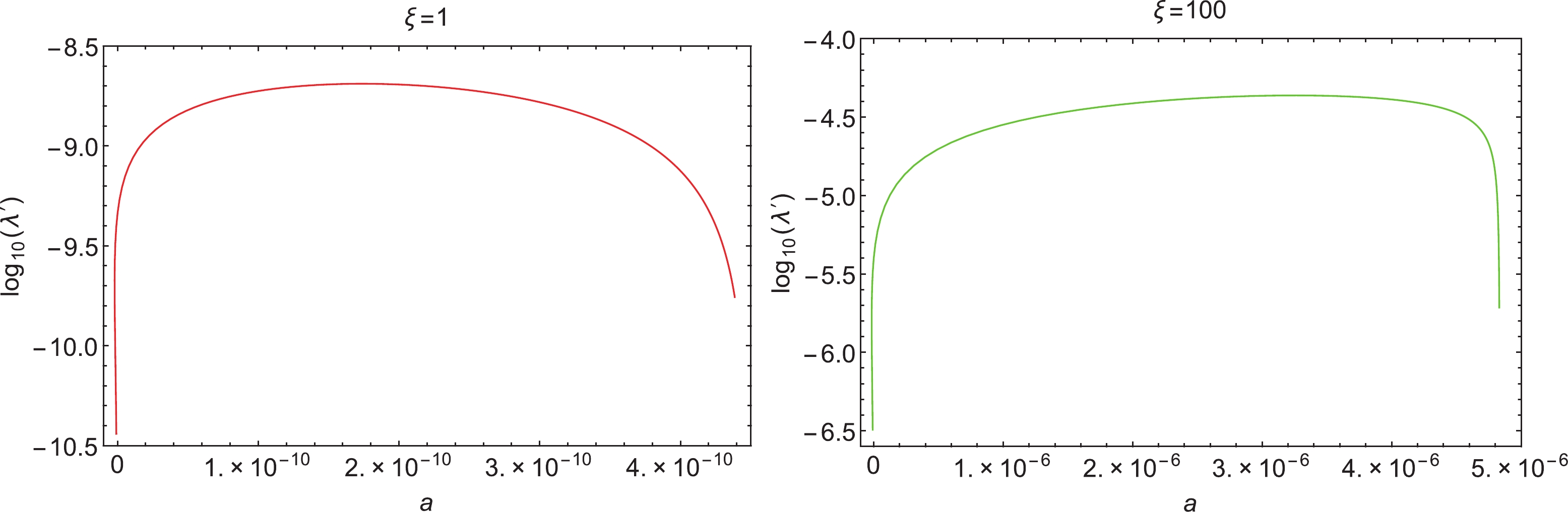
Figure 2. (color online)
$ \log_{10}(\lambda^\prime) $ vs. a for$ \xi = 1 $ (left) and$ \xi = 100 $ (right).The amount of expansion from the horizon crossing moment up to the end of inflation is quantified by the number of e-folds:
$ N = -\frac{1}{M^2_P}\int_{\Delta^0_{*}}^{\Delta^0_f}\frac{V(\Delta^0)}{V^\prime(\Delta^0)}\left(\frac{{\rm d}\chi}{{\rm d}\Delta^0}\right)^2{\rm d}\Delta^0. $

(29) In the non-minimal inflationary scenario with a relatively small coupling to gravity,
$ \xi \lesssim 100 $ , the reheating process occurs predominantly as in a radiation dominated universe [64-67]. As pointed out in [66], the e-folds number can be estimated to be approximately 60 in these cases. Using$ N = 60 $ , we can solve Eq. (29) for the field strength at horizon crossing,$ \Delta^0_{*} $ .Finally, we can use the expressions in Eq. (27) to calculate the predictions of our model for
$ n_S $ and r parameters. Fig. 3 shows our results in the$ n_S \times r $ plane. Note that the predictions are in good agreement with the observations, even though$ \xi \leqslant 100 $ . In particular, for$ \xi = 100 $ and$ a = 0 $ , we obtain$ n_S\simeq 0.968 $ and$ r\simeq 3 \times 10^{-3} $ , well inside the 68% CL contour of the Planck2018 data set. Moreover, we have a unitarily safe model, as inflation takes place in an energy scale$ H_{*} = \sqrt{V_{*}/3M^2_P} \simeq 1.38 \times 10^{13} $ GeV, well bellow the unitarity scale$ \Lambda_U = \dfrac{M_P}{\xi}\sim 2.435 \times 10^{16} $ GeV.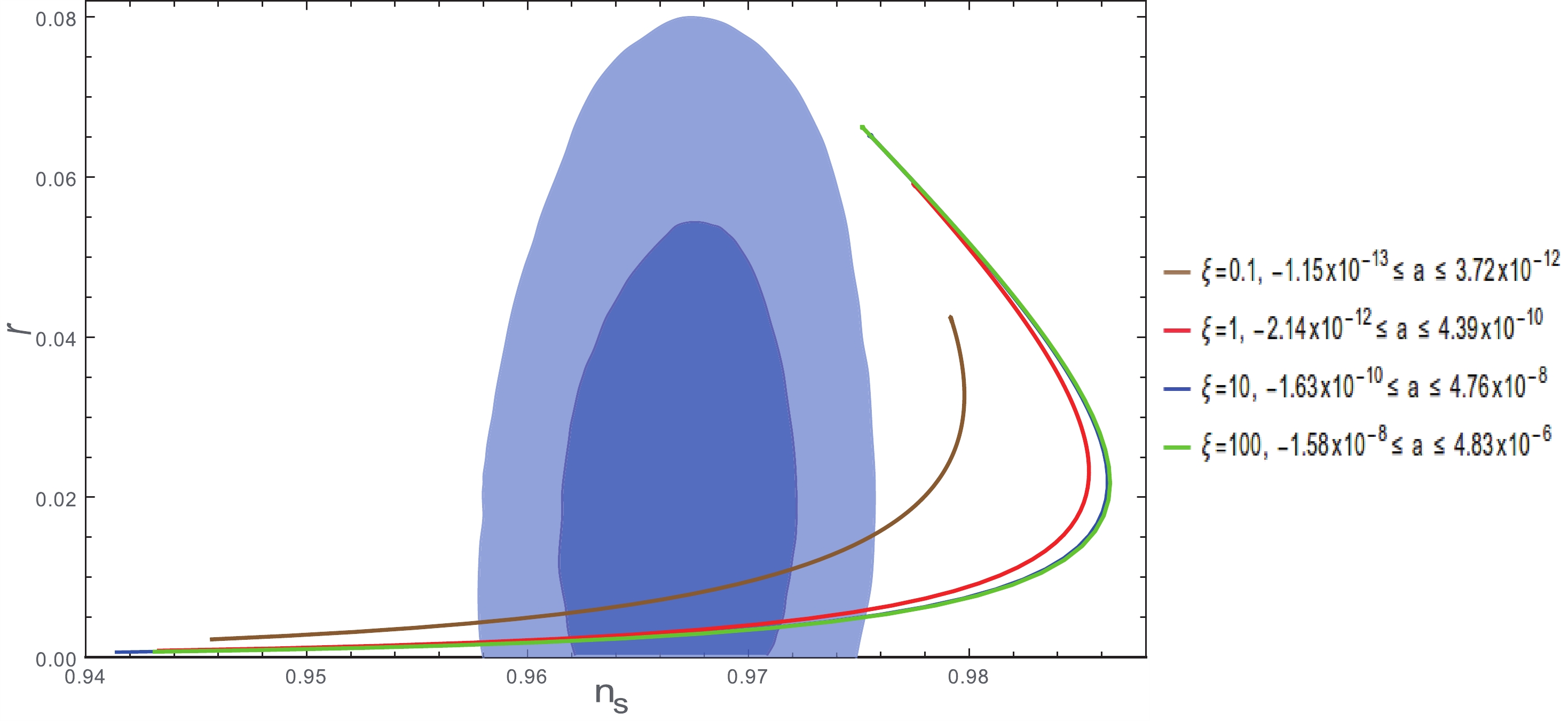
Figure 3. (color online)
$ n_S $ vs. r for$ \xi = 0.1 $ ,$ 1 $ ,$ 10 $ , and$ 100 $ . The grey areas show the regions favoured by Planck2018, with 68% and 95% confidence levels (Planck$TT,TE,EE+{\rm low} E+{\rm lensing}+BK14+BAO$ data set [9]). The intervals considered for the radiative corrections are also shown, being the lower (upper) limit in a responsible for the lower (upper) end of each curve.However, the most interesting result comes from the possibility to constrain the parameters of the Lagrangian through the inflationary observable. For
$ \xi = 100 $ , one may require$ -1.11\times 10^{-8} \lesssim a \lesssim 1.22 \times 10^{-8} $ to obtain the predictions of the model in accordance with the Planck observations (68% CL). Following Eq. (23), one could use these bounds to constrain the couplings contributing to radiative corrections, including the Yukawa and gauge couplings ($ Y_{\nu_i} $ and$g_{\rm B-L}$ ), associated to the physics beyond the standard model. Certainly, a vast computational effort would be necessary to estimate the impact of these bounds in the neutrino physics or search for a new gauge boson. Given that Eq. (22) evaluates the radiative corrections on the renormalization scale$ M_P $ , the application of Renormalization Group equations would be mandatory to obtain the corresponding bounds at energy scales accessible to low energy experiments (oscillation and collider experiments). We will consider this analysis in a forthcoming communication.After the inflationary period, the inflaton oscillates around its vev, giving rise to the reheating phase [68-70]. Owing to its mass structure, the inflaton is massive enough to decay in pairs of gauge bosons, neutrinos, or even the Higgs field. Even before the inflaton settles at its vev, non-perturbative effects could take place, producing gauge bosons [39, 71]. In this case, the scenario is significantly more complicated, and numerical study in lattice is mandatory.
-
We remark that, in the B-L model proposed here, the masses of the standard neutrinos are achieved through an adapted type II seesaw mechanism. In view of this, the following question arises: what are the reasons for the existence of the RHNs in the model? The immediate answer is that they are required to cancel gauge anomalies. In addition, they may compose the dark matter content of the universe in the form of WIMP.
Although the three RHNs are potentially DM candidates, for simplicity reasons, we only consider that the lightest one, which we call N, is sufficient to provide the correct relic abundance of DM of the universe in the form of WIMP. This means that N was in thermal equilibrium with the SM particles in the early universe. Then, as far as the universe expands and cools, the thermal equilibrium is lost, causing the freeze out of the abundance of N. This takes place when the N annihilation rate, whose main contributions are displayed in Fig. 4, becomes roughly smaller then the expansion rate of the universe. In this case, the relic abundance of N is obtained by evaluating the Boltzmann equation for the number density
$ n_N $ ,
Figure 4. Main contributions to the DM relic abundance. The SM contributions stand for fermions, Higgs, and vector bosons.
$ \frac{{\rm d} n_N}{{\rm d}t}+3H n_N = -\langle\sigma v\rangle(n_N^2 - n_{\rm{EQ}}^2), $

(30) where
$ \begin{align} H^2 \equiv \left( \frac{\dot{a}}{a} \right)^2 = \frac{8 \pi }{3M_P^2} \rho , \end{align} $

(31) with
$ n_{\rm{EQ}} $ and$ a(t) $ being the equilibrium number density and the scale factor, respectively, in a situation where the radiation dominates the universe with the energy density$ \rho = \rho_{\rm{rad}} $ , i.e., the thermal equilibrium epoch. Note that$ \langle\sigma v\rangle $ is the thermal average product of the annihilation cross section times the relative velocity [11]. As usually adopted, we present our results in the form of$ \Omega_N $ , which is the ratio between the energy density of N and the critical density of the universe.We proceeded as follows. We numerically analyzed the Boltzmann equation by using the micrOMEGAs software package (v.2.4.5) [72]. To this end, we implemented the model in Sarah (v.4.10.2) [73-76] in combination with SPheno (v.3.3.8) [77, 78] package, which solves all mass matrices numerically. Our results for the relic abundance of N are displayed in Fig. 5. The thick lines in those plots correspond to the correct abundance. Note that, although the Yukawa coupling
$ Y_{N} $ is an arbitrary free parameter that translates in N developing any mass value, the key point to determine whether the model provides the correct abundance of N is the resonance of$ Z^{\prime} $ and H. This is showed in the top left plot in Fig. 5. In this plot, the first resonance corresponds to a$ Z^{\prime} $ with mass around$ 3 $ TeV, and the second resonance corresponds to H with mass in the range from$ 6 $ TeV up to$ 7 $ TeV. In the top right plot, we show the density of DM varying with its mass, but now including the region excluded by the LEP constraint expressed in Eq. (8). On the bottom left plot of Fig. 5, we zoom in on the resonance of H. Note that we included the LEP constraint. For completeness reasons, on the bottom right plot, we show the dependence of$ M_{Z^{\prime}} $ with$g_{\rm B-L}$ , including the LEP exclusion region and LHC constraint [79] as well. In the last three plots, we show two benchmark points localized exactly in the line that gives the correct abundance. They are represented in red square and orange star points, and their values are displayed in the companion table. Observe that the LEP constraint in Eq. (8) imposes a reasonably massive N with mass in the range of a few TeVs. To complement these plots, we show another in Fig. 7 that relates the resonance of H (all points in color) and the mass of the DM. The mixing parameter$ \sin \theta $ is given in Eq. (11). Observe that LEP exclusion derived from Eq. (8) is a very stringent constraint imposing H with mass above$ 5800 $ GeV and requiring DM with mass above$ 2800 $ GeV. All those points in colors provide the correct abundance, but only those in black recover the standard Higgs with mass of$ 125 $ GeV. The benchmark points in red square and orange star are given in Table 1. In summary, for the range of values chosen for the parameters, N with mass around 3 TeV constitutes a viable DM candidate, once it provides the correct relic abundance required by the experiments [9]. Moreover, a viable DM candidate must obey the current direct detection constraints.MDM/GeV YN1 $ M_{Z^\prime} $ /GeV

gB-L MH/GeV $ \Omega h^2 $ 

vS $\sigma_{{\rm DM}q}$ 

q 3050 0.291 3840 0.518 6279 0.116 7400 5.4 10-11 ★ 3190 0.294 3904 0.509 6470 0.122 7658 5.4304e-11 ■ Table 1. (color online) Benchmark points for parameters values added on plots.

Figure 5. (color online) Plots relating DM relic abundance, Yukawa coupling of the RHN, and the dark matter candidate mass. The thick horizontal line corresponds to the correct relic abundance [9].
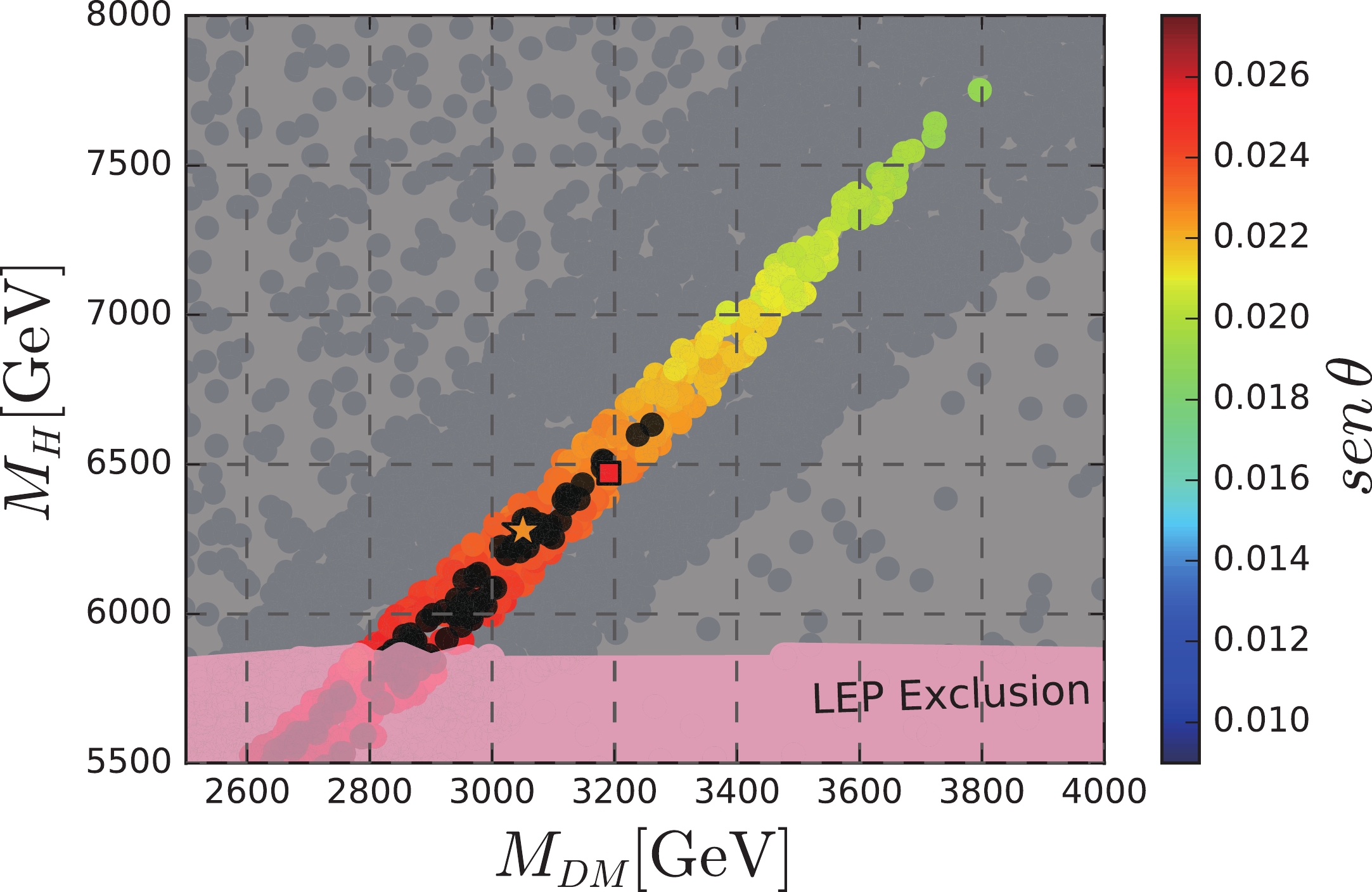
Figure 7. (color online) Physical parameter space of
$M_{H_2}\times M_{\rm DM}$ . In colors we show the points that provide the correct relic abundance in the resonant production of the singlet scalar, in accordance with the diagrams in Fig. 4. The black points recover a Higgs with mass of$ 125 $ GeV.In addition to the relic density of the DM candidate, which involves gravitational effects, we only need to detect it directly to reveal its nature. Here, we restricted our study to direct detection. Aiming to detect the signal of DM directly in the form of WIMPs, many underground experiments using different types of targets were conducted. Unfortunately, no signal has been detected yet. The results of such experiments translate into upper bounds for the WIMP-Nucleon scattering cross section. In view of this, any DM candidate in the form of WIMPs must be subjected to the current direct detection constraints. Direct detection theory and experimentation constitute a very well developed topic in particle physics. For a review of the theoretical predictions for direct detection of WIMPs in particle physics models, please refer to [80-82]. For a review of experiments, refer to [83]. In our case, direct detection requires interactions among N and quarks. This is achieved by exchange of h and H via t-channel, as displayed in Fig. 6. Note that
$ Z^{\prime} $ t-channel constitutes a very suppressed contribution because N is a Majorana particle [84]. Consequently, we dismissed such contributions here. In practical terms, we need to obtain the WIMP-quark scattering cross section reported in [85]. Note that the scattering cross section is parameterized by four free parameters, namely$ M_N $ ,$ M_H $ ,$ v_S $ , and the mixing angle$ \theta $ given in Eq. (11). However, this cross section depends indirectly on other parameters. For example, for$g_{\rm B-L}$ in the range$ 0.1 - 0.55 $ , the LEP constraint in Eq. (8) implies$ v_S > 7 $ TeV and$ M_{Z^{\prime}} $ around$ 3 $ TeV. Considering this, and using the micrOMEGAs software package [72] in our calculations, we present our results for the WIMP-Nucleon cross section in Fig. 8. All color points led to the right abundance and are in accordance with the Xenon (2018) exclusion bound [86]. The points in pink are excluded by the LEP constraint provided in Eq. (8). However, only those points in black recover a Higgs with mass of 125 GeV. Observe that the black points may be probed by future XenonNnT and DarkSide direct detection experiments. This turns our model into a phenomenological viable DM model.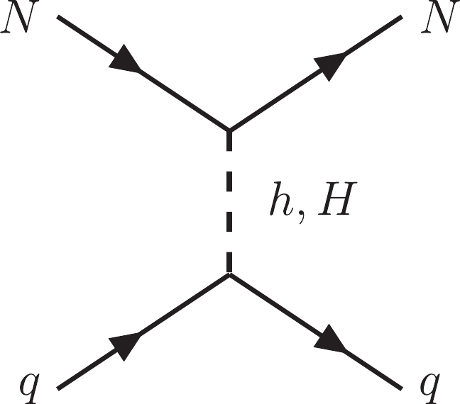
Figure 6. The WIMP-quark scattering diagram for direct detection.

Figure 8. (color online) Spin-independent (SI) WIMP-nucleon cross sections constraints. The lines correspond to experimental upper limit bounds on direct detection for LUX [87] (black line), current Xenon1T [86] (blue line with blue fill area), Xenon1T [88] (green dashed line, prospect, 2t
$ \cdot $ y exposure), XenoNnT [88] (prospect, 20t$ \cdot $ y exposure, purple line), Dark Side Prospect [89] (red dashed and dark red dashed lines for different exposure times), LUX-Zeppelin Prospect [90] (orange dashed line), and the neutrino coherent scattering, atmospheric neutrinos and diffuse supernova neutrinos [91] (orange dashed line with filled area). -
In this study, the type II seesaw mechanism for generation of small neutrino masses was implemented within the framework of the B-L gauge model. We showed that neutrino masses at eV scale require that
$ \Delta $ belongs to an energy mass scale around$ 10^9 $ GeV. This characterizes a seesaw mechanism at an intermediate energy scale and can be probed through rare lepton decays.One interesting advantage of this model is that we can evoke a
$ Z_2 $ discrete symmetry and leave the right-handed neutrinos completely dark in relation to the standard model interactions. In this case, the neutrinos turn out to be the natural candidate for the dark matter of universe in the form of WIMP. We also showed that the correct abundance of dark matter is obtained owing to the resonant production of$ Z^{\prime} $ and heavy Higgs H. Although our scenario is in accordance with Xenon1T exclusion bound, the prospect is that direct detection experiments will be able to probe it.Concerning inflation, by allowing a non-minimal coupling of the neutral component of the scalar triplet with gravity, we showed that the model realizes inflation in a very successful way, given that the model accommodates Planck results for inflationary parameters in a scenario where the loss of unitarity occurs orders of magnitude above the energy density during inflation. An interesting possibility arises from the estimation of the Lagrangian parameters through the inflationary observable. Future observations of the B-mode polarization, such as LiteBIRD [92], may improve the constraints over the inflationary parameters and, consequently, the Lagrangian. We shall consider this analysis in a forthcoming communication.
-
The authors would like to thank Clarissa Siqueira and P. S. Rodrigues da Silva for helpful suggestions.
Neutrino masses, cosmological inflation and dark matter in a variant U(1)B-L model with type II seesaw mechanism
- Received Date: 2020-07-18
- Accepted Date: 2020-11-29
- Available Online: 2021-02-15
Abstract: In this study, we implemented the type II seesaw mechanism into the framework of the


 DownLoad: