


 Abstract
 HTML
HTML Reference
 Related
 PDF
PDF


-
Research into exotic hadrons that are composed of multi-quark states is among the current subjects of interest in particle physics. Experimental information collected through various collaborations, and theoretical progress obtained using different theoretical models, constitutes the rapidly growing field of exotic studies [1-10]. In 2015, the LHCb Collaboration reported two pentaquark states,
$ P_c^+(4380) $ and$ P_c^+(4450) $ , in the invariant mass spectrum of$ J/\psi\,p $ in the$ \Lambda_b^0 \rightarrow J/\psi\,K^-\,p $ decay [11]. From the LHCb measurements the$ P_c^+(4380) $ has a mass of$ 4380 \pm 8 \pm 29 $ MeV and a width of$ 205 \pm 18 \pm 86 $ MeV, while the$ P_c^+(4450) $ has a mass of$ 4449.8 \pm 1.7 \pm 2.5 $ MeV and a width of$ 39 \pm 5 \pm 19 $ MeV. The quantum numbers of these states were determined by partial wave analysis and the spins reported as$ 3/2 $ and$ 5/2 $ with opposite parities. In 2019, the LHCb Collaboration updated their analysis and reported three new narrow pentaquark states [12]. The measured masses and decay widths are:$ \begin{aligned}[b] P_c(4312): \ M = &\, 4311.9 \pm 0.7 ^{+6.8}_{-0.6},\\ \Gamma = &\, 9.80 \pm 2.7^{+3.7}_{-4.5},\\ P_c(4440): \ M= &\, 4440.3 \pm 1.3 ^{+4.1}_{-4.7},\\ \Gamma = &\, 20.6 \pm 4.9^{+8.7}_{-10.1},\\ P_c(4457): \ M= &\, 4457.3 \pm 0.6 ^{+4.1}_{-1.7},\\ \Gamma = &\, 6.40 \pm 2.0^{+5.7}_{-1.9}. \end{aligned} $

All values are given in units of MeV. From the updated measurements, we observe that the previous peak of
$ P_c(4450) $ is now split into two narrower structures,$ P_c(4440) $ and$ P_c(4457) $ , and a fluctuation observed in the old spectrum is now a new narrow resonance,$ P_c(4312) $ . The broad$ P_c(4380) $ resonance is now less clear and its existence needs to be verified in a complete amplitude analysis. One can see that the$ P_c(4312) $ is just below the$ \Sigma_c \bar D $ threshold, while the masses of the$ P_c(4440) $ and$ P_c(4457) $ are slightly lower than the$ \Sigma_c \bar D^{*} $ threshold. Since these states have only been observed in the$ J/\psi p $ invariant mass spectrum by the LHCb Collaboration, it is important to investigate some other decay mechanisms to better understand their internal structure. The experimental discovery stimulated extensive theoretical predictions on the nature of pentaquark states, their spectroscopic parameters, decays and production mechanisms, employing different scenarios and frameworks [13-45]. The majority of these studies are aimed at understanding the spectroscopy and decay properties of these particles, and the results obtained using different models are close to each other. To put it another way, the spectroscopic parameters or decay properties alone cannot distinguish the substructure of the pentaquark states. Therefore, additional investigations of these pentaquark states are required to explain the situation with the pentaquark resonances.The magnetic moment of hadrons is one of the most significant properties in the study of their electromagnetic structure, and can also give important knowledge of the QCD dynamics in the low energy region. It is also a key component in the computation of
$ J/\psi $ photo-production cross sections, which can ensure an independent investigation of the pentaquark states. In this work, we focus all our attention on the newly discovered$ P_c(4312) $ state (from now on we denote this particle as$ P_c $ ) and perform a comprehensive calculation of the magnetic moment of the$ P_c $ with the external background electromagnetic field method. We use the light-cone QCD sum rule (LCSR) method, which is one of the most powerful and useful nonperturbative methods in hadron physics, allowing us to calculate properties of particles and processes [46-48]. In the calculations, we use the diquark-diquark-antiquark and molecular forms of the interpolating currents for the$ P_c $ pentaquark and the distribution amplitudes of the photon, which contain all knowledge about the nonperturbative dynamical features of the photon. Studying the electromagnetic properties of exotic states is a relatively new subject. However, in the literature there are a few studies where the electromagnetic properties of the hidden-charm pentaquark states are investigated [49-51]. In Ref. [49], the magnetic moments of the hidden-charm pentaquark states have been extracted in the diquark-triquark, diquark-diquark-antiquark and molecular configurations with$J^P = \dfrac{1}{2}^{\pm}, \dfrac{3}{2}^{\pm}, \dfrac{5}{2}^{\pm} \rm{and}\; \dfrac{7}{2}^{+}$ quantum numbers in difcolor-flavor structures. In Ref. [50], the electromagnetic multipole moments of the$ P_c(4380) $ pentaquark with$J^P = \dfrac{3}{2}^{-}$ quantum numbers have been obtained in the diquark-diquark-antiquark and molecular pictures within the LCSR framework. In Ref. [51], the ground statesof hidden-charm pentaquarks with$J^P = \dfrac{3}{2}^{-}$ quantum numbers and their associated magnetic moments and electromagnetic couplings were acquired, of interest to pentaquark photoproduction experiments in the framework of the constituent quark model. We see that from these studies the values of the electromagnetic parameters obtained via different configurations differ considerably from each other.The rest of this paper is structured as follows. In Section II, we describe how to evaluate the magnetic moment of the
$ P_c $ pentaquark with the LCSR. In Section III, we carry out numerical analysis of the acquired LCSR for the magnetic moment of the$ P_c $ pentaquark state. This section contains also our discussion. Section IV gives a summary and outlook. The explicit expressions of the magnetic moment are in the Appendix. -
In this section, we briefly describe the LCSR method used to investigate the magnetic moment of the
$ P_c $ pentaquark state in the presence of an external electromagnetic field. The current correlation function for the$ P_c $ pentaquark state is written as$ \Pi(p,q) = {\rm i}\int {\rm d}^{4}x{\rm e}^{{\rm i}p\cdot x}\langle 0|\mathcal{T}\{J_{P_c}(x) \bar J_{P_c}(0)\}|0\rangle_{\gamma}, $

(1) where
$ J_{P_c}(x) $ is the interpolating current of the$ P_c $ pentaquark. In the diquark-diquark-antiquark and molecular pictures with quantum numbers$ J^P = \dfrac{1}{2}^- $ , it is given as [27, 28]$ \begin{aligned}[b] J^{\rm Di}(x) =& \varepsilon^{abc}\varepsilon^{ade}\varepsilon^{bfg}\big[ u^T_d(x) C\gamma_5 d_e(x)\,u^T_f(x) \\ &\times C\gamma_5 c_g(x)\, C\bar{c}^{T}_{c}(x)\big],\\ J^{\rm Mol}(x) = &\big[\bar{c}_{d}(x){\rm i} \gamma_{5}u_{d}(x)\big] \big[\epsilon^{abc}(u_{a}^{T}(x)C\gamma_{\alpha} d_{b}(x))\\ &\times \gamma^{\alpha}\gamma_{5}c_{c}(x)\big], \end{aligned} $

(2) where
$ C $ is the charge conjugation matrix, and$ a $ ,$ b $ ... are colour indices.The correlation function can be acquired associated with hadronic properties, known as the hadronic representation. It can also be acquired associated with the quark-gluon properties in the deep Euclidean region, known as the QCD representation. In order to eliminate the undesired contributions coming from the higher states and the continuum, we perform a Borel transformation and continuum subtraction, provided by the quark-hadron duality ansatz. Finally, both representations of the correlation function are connected to each other via dispersion relations.
The hadronic representation of the correlation function can be acquired by embedding complete sets of the hadronic states with the same quantum numbers as the
$ {P_c} $ interpolating currents,$ \begin{aligned}[b] \Pi^{\rm Had}_{\mu\nu}(p,q)= &\frac{\langle0\mid J_{P_c} \mid {P_c}(p, s)\rangle}{[p^{2}-m_{{P_c}}^{2}]}\langle {P_c}(p, s)\mid {P_c}(p+q, s)\rangle_\gamma \\ &\times \frac{\langle {P_c}(p+q, s)\mid \bar{J}_{P_c} \mid 0\rangle}{[(p+q)^{2}-m_{{P_c}}^{2}]}+..., \end{aligned} $

(3) where the ellipsis represents the continuum and higher states.
The matrix elements
$ \langle0\mid J_{P_c}\mid {P_c}(p, s)\rangle $ ,$\langle {P_c}(p+q, s)\mid \bar J_{P_c}\mid 0\rangle$ and$ \langle {P_c}(p, s)\mid {P_c}(p+q, s)\rangle_\gamma $ in Eq. (3) can be parameterized in terms of overlap amplitude and Lorentz invariant form factors as follows:$ \begin{array}{l} \langle0\mid J_{P_c}\mid {P_c}(p, s)\rangle = \lambda_{P_c} \gamma_5 \, u(p,s), \end{array} $

(4) $ \begin{array}{l} \langle {P_c}(p+q, s)\mid\bar J_{P_c}\mid 0\rangle = \lambda_{P_c} \gamma_5 \, \bar u(p+q,s), \end{array} $

(5) $ \begin{aligned}[b] \langle {P_c}(p, s)\mid {P_c}(p+q, s)\rangle_\gamma = &\varepsilon^\mu\,\bar u(p, s)\Biggr[\big[f_1(q^2)+f_2(q^2)\big] \gamma_\mu \\ &+f_2(q^2) \dfrac{(2p+q)_\mu}{2 m_{P_c}}\Biggr]\,u(p+q, s) , \end{aligned} $

(6) where
$ \lambda_{P_c} $ is the residue or overlap amplitude of the$ P_c $ state, and$ \varepsilon $ and q are the polarization vector and momentum of the photon, respectively.Substituting Eqs. (4)-(6) in Eq. (3), for the hadronic side we get:
$ \begin{aligned}[b] \Pi^{\rm Had}(p,q) =& \lambda^2_{P_c}\gamma_5 \frac{\Big({\not\!\! p } +m_{P_c} \Big)}{[p^{2}-m_{{P_c}}^{2}]}\varepsilon^\mu \Biggr[\big[f_1(q^2)+f_2(q^2)\big] \gamma_\mu \\ &+f_2(q^2)\, \frac{(2p+q)_\mu}{2 m_{P_c}}\Biggr] \gamma_5 \frac{\Big({\not\!\! p } +{\not\!\! q } +m_{P_c}\Big)}{[(p+q)^{2}-m_{{P_c}}^{2}]}. \end{aligned} $

(7) The Lorentz invariant form factors
$ f_1(q^2) $ and$ f_2(q^2) $ are related to the magnetic form factor by the relation$ \begin{array}{l} G_M(q^2) = f_1(q^2)+f_2(q^2). \end{array} $

(8) At
$ q^2 = 0 $ , the magnetic form factor is acquired associated with the functions$ f_1(q^2) $ and$ f_2(q^2) $ as:$ \begin{array}{l} G_M(0) = f_1(0)+f_2(0). \end{array} $

(9) The magnetic moment,
$ \mu_{P_c} $ , is defined in the following way:$ \begin{array}{l} \mu_{P_c} = G_M(0) \, \dfrac{e}{2\,m_{P_c}}. \end{array} $

(10) We notice from Eq. (7) that the correlation function includes many structures. Any of these can be selected in evaluating the magnetic moment of the
$ P_c $ pentaquark, and from this point of view we select the structure${\not\!\! \varepsilon }{\not\!\! q}$ . This structure contains the magnetic form factor$ f_1(0) + f_2(0) $ , and it gives the magnetic moment$ \mu_{P_c} $ of the$ P_c $ pentaquark in units of its natural magneton, i.e.$ e/2\,m_{P_c} $ . As a result, the correlation function can be expressed with respect to the magnetic moment of the$ P_c $ pentaquark as:$ \Pi^{\rm Had}(p,q)= \frac{\lambda^2_{P_c}\,m_{P_c}}{[(p+q)^2-m^2_{P_c}]} \,\mu_{P_c}\, \frac{1}{[p^2-m^2_{P_c}]}. $

(11) Employing the explicit form of the interpolating currents given in Eq. (2), and after some lengthy computations, for the QCD representation of the correlation function of the
$ P_c $ pentaquark we obtain:$ \begin{aligned}[b] \Pi_1^{\rm QCD}(p,q) =& -{\rm i}\,\varepsilon^{abc}\varepsilon^{a^{\prime}b^{\prime}c^{\prime}}\varepsilon^{ade} \varepsilon^{a^{\prime}d^{\prime}e^{\prime}}\varepsilon^{bfg} \varepsilon^{b^{\prime}f^{\prime}g^{\prime}}\\ &\times\int {\rm d}^4x {\rm e}^{{\rm i}p\cdot x} \langle 0| \Bigg\{ {\rm Tr}\Big[\gamma_5 S_d^{ee^\prime}(x) \gamma_5 \tilde S_u^{dd^\prime}(x)\Big] \\ &\times {\rm Tr}\Big[\gamma_5 S_c^{gg^\prime}(x) \gamma_5 \tilde S_u^{ff^\prime}(x)\Big] \\ &- {\rm Tr} \Big[\gamma_5 S_d^{ee^\prime}(x) \gamma_5 \tilde S_u^{fd^\prime}(x) \gamma_5 S_c^{gg^\prime}(x) \\ &\times \gamma_5 \tilde S_u^{df^\prime}(x)\Big] \Bigg \} \tilde S_c^{c^{\prime}c}(-x) |0 \rangle_\gamma , \end{aligned} $

(12) in the diquark-diquark-antidiquark picture, and
$ \begin{aligned}[b] \Pi_2^{\mathrm{QCD}}(p,q) =& -{\rm i}\,\epsilon^{abc}\epsilon^{a^{\prime}b^{\prime}c^{\prime}}\,\int {\rm d}^{4}x{\rm e}^{{\rm i}p\cdot x}\\ &\times \langle 0| \Bigg\{\mathrm{Tr}\Big[\gamma_{5} S_{u}^{dd^{\prime}}(x) \gamma_{5}S_c^{d^{\prime}d}(-x)\Big]\\ &\times \mathrm{Tr}\Big[\gamma_{\beta}\widetilde{S}_u^{aa^{\prime}}(x)\gamma_{\alpha}S_d^{bb^{\prime}}(x) \Big] \\ &- \mathrm{Tr}\Big[\gamma_{5} S_{u}^{dd^{\prime}}(x) \gamma_{5} S_c^{d^{\prime}d}(-x) \Big]\\ &\times \mathrm{Tr}\Big[\gamma_{\beta}\widetilde{S}_{u}^{ba^{\prime}}(x)\gamma_{\alpha}S_d^{ab^{\prime}}(x)\Big] \Bigg \}\\ &\times \Big( \gamma^{\alpha}\gamma_{5}S_c^{cc^{\prime}}(x)\gamma_{5}\gamma^{\beta}\Big) |0 \rangle_\gamma, \end{aligned} $

(13) in the molecular picture, where
$ \widetilde{S}_{c(q)}^{ij}(x) = CS_{c(q)}^{ij\mathrm{T}}(x)C, $

with
$ S_{q(c)}(x) $ being the full light and charm quark propagators. The relevant propagators are given as [52]$ \begin{aligned}[b] S_{q}(x)= &{\rm i} \frac{{\not\!\! x }}{2\pi ^{2}x^{4}} - \frac{ \bar qq }{12} - \frac{ \bar q \sigma. G q }{192} x^2\\ &-\frac {{\rm i} g_s }{32 \pi^2 x^2} G^{\mu \nu}(x) \Bigg[\rlap/{x} \sigma_{\mu \nu} + \sigma_{\mu \nu} \rlap/{x} \Bigg], \end{aligned} $

(14) $ \begin{aligned}[b] S_{c}(x)= & \frac{m_{c}^{2}}{4 \pi^{2}} \Bigg[ \frac{K_{1}\Big(m_{c}\sqrt{-x^{2}}\Big) }{\sqrt{-x^{2}}} +{\rm i}\frac{{\not\!\! x }\; K_{2}\Big( m_{c}\sqrt{-x^{2}}\Big)} {(\sqrt{-x^{2}})^{2}}\Bigg]\\ &-\frac{g_{s}m_{c}}{16\pi ^{2}} \int_0^1 {\rm d}v\, G^{\mu \nu }(vx)\Bigg[ (\sigma _{\mu \nu }{\not\!\! x } +{\not\!\! x }\sigma _{\mu \nu })\\ &\times \frac{K_{1}\Big( m_{c}\sqrt{-x^{2}}\Big) }{\sqrt{-x^{2}}} +2\sigma_{\mu \nu }K_{0}\Big( m_{c}\sqrt{-x^{2}}\Big)\Bigg]. \end{aligned} $

(15) where
$ K_i $ are the modified second order Bessel functions and$ G^{\mu\nu} $ is the gluon field strength tensor.The QCD representation of the correlation function can be acquired with respect to the quark-gluon properties with the help of the photon distribution amplitudes and after performing a Fourier transformation to transfer the computations to momentum space. These procedures are standard in the LCSR method but quite lengthy. Therefore, we do not present these steps here.
Equating the QCD and hadronic representations of the correlation function, we acquire the terms of the magnetic moment in the LCSR associated with the QCD degrees of freedom and the photon distribution amplitudes. We carry out double Borel transforms in connection with the variables
$ p^2 $ and$ (p + q)^2 $ on both representations of the correlation function to remove the contributions of the higher states and continuum, and employ the quark-hadron duality ansatz. By equating the coefficients of the structure${\not\!\! \varepsilon }{\not\!\! q}$ for the magnetic moment, we obtain:$ \mu^{\rm Di}_{P_c} = G_M^{\rm Di}(0) \frac{e}{2 m_{P_c}} = \frac{{\rm e}^{\frac{m^2_{P_c}}{M^2}}}{\lambda^2_{P_c}\, m_{P_c}}\, F_1^{\rm QCD}, $

(16) $ \mu^{\rm Mol}_{P_c} = G_M^{\rm Mol}(0) \frac{e}{2 m_{P_c}} = \frac{{\rm e}^{\frac{m^2_{P_c}}{M^2}}}{\lambda^2_{P_c}\, m_{P_c}}\, F_2^{\rm QCD}. $

(17) The explicit expressions of the
$ F_1^{\rm QCD} $ and$ F_2^{\rm QCD} $ functions are presented in the Appendix. Interested readers can find details of the calculations, such as the Borel transformations and continuum subtraction, in Refs. [53, 54]. -
This section is dedicated to the numerical computations for the magnetic moment of the
$ P_c $ pentaquark state. We use$ m_u = m_d = 0 $ ,$ m_c = 1.27 \pm 0.03\,\rm{GeV} $ [55],$ m_{P_c} = 4.31 \pm 0.07\; \rm{GeV} $ [12],$ \langle \bar uu\rangle = \langle \bar dd\rangle = (-0.24 \pm 0.01)^3\,\rm{GeV}^3 $ ,$m_0^{2} = 0.8 \pm 0.1 \,\rm{GeV}^2$ [56],$ \langle g_s^2G^2\rangle = 0.88\; \rm{GeV}^4 $ [57]. We also need the value of the magnetic susceptibility, which is taken as$ \chi = -2.85 \pm 0.5\; \rm{GeV}^{-2} $ [58]. In order to evaluate a numerical estimation for the magnetic moment, we also need to determine the numerical values of the residue of the$ P_c $ pentaquark. The residue is acquired from the two-point sum rule as$ \lambda_{P_c} = (1.95 \pm 0.35)\times 10^{-3}\; \rm{GeV}^6 $ [28],$ \lambda_{P_c} = (1.40 \pm 0.23)\times 10^{-3}\; \rm{GeV}^6 $ [27] for molecular picture and the diquark-diquark-antiquark picture, respectively. The analytical expressions used in the photon distribution amplitudes and the numerical values used in these expressions are given in Ref. [59].The predictions for the magnetic moment of the
$ P_c $ pentaquark state depend on two auxiliary parameters: the Borel mass parameter$ M^2 $ and the continuum threshold$ s_0 $ . According to the standard prescriptions of the method used, the physical parameters should weakly depend on these auxiliary parameters. The upper bound of$ M^2 $ is achieved by demanding the maximum pole contributions, and its lower bound is achieved from the convergence of the operator product expansion and the excess of the perturbative part over nonperturbative contributions.The working region for$ s_0 $ is achieved by considering the fact that the magnetic moment is practically insensitive to its changes. The above-mentioned constraints result in the working regions for arbitrary parameters being:$ \begin{aligned}[b] &22.0\; \rm{GeV}^2 \leqslant s_0 \leqslant 24.0\; \rm{GeV}^2,\\ &5.0\; \rm{GeV}^2 \leqslant M^2 \leqslant 7.0\; \rm{GeV}^2. \end{aligned} $

In Fig. 1, we depict the dependencies of the magnetic moment on
$ M^2 $ and$ s_0 $ . The uncertainty because of variations of$ s_0 $ in this range is much larger than the uncertainty because of variations of$ M^2 $ . Note that the specified interval of$ s_0 $ is in the interval that one would assume from the physical analysis of$ s_0 $ . As a result of all these considerations we obtain for the magnetic moment: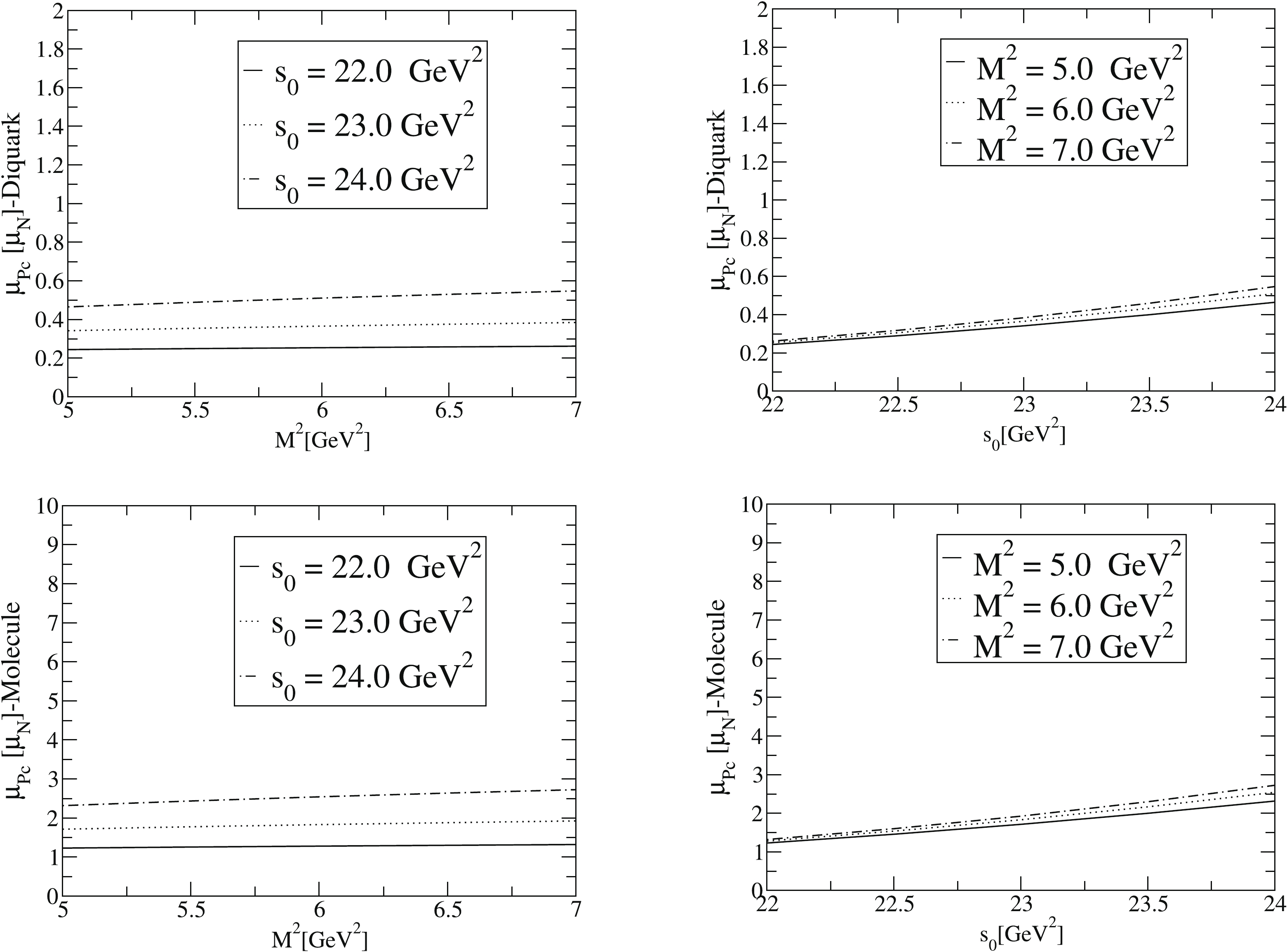
Figure 1. Variations of the magnetic moment
$ \mu_{P_c} $ with$ M^2 $ and$ s_0. $ $ \begin{aligned}[b] \mu_{P_c}^{\rm Di} =& G_M^{\rm Di}(0) \frac{e}{2 m_{P_c}} = 1.82 \pm 0.70 \,\, \frac{e}{2 m_{P_c}} \\ =& 0.40 \pm 0.15\; \mu_N, \end{aligned} $

(18) $ \begin{aligned}[b] \mu_{P_c}^{\rm Mol} =& G_M^{\rm Mol}(0) \frac{e}{2 m_{P_c}} = 9.09 \pm 3.44 \, \, \frac{e}{2 m_{P_c}} \\ =& 1.98 \pm 0.75\; \mu_N, \end{aligned} $

(19) where
$ \mu_N $ is the nucleon magneton.Our numerical values clearly indicate that the magnetic moment of the pentaquark state is quite different when obtained with different models. To put it another way, the experimental measurement of the magnetic moment of the
$ P_c $ pentaquark can actually help distinguish its substructure. In Ref. [49], the magnetic moment of the hidden-charm pentaquark states have been extracted in the diquark-triquark, diquark-diquark-antiquark and molecular configuration with different quantum numbers. Our predictions are in good agreement, within the errors, with the predictions of Ref. [49]. -
In 2019, the LHCb Collaboration reported the observation of three narrow new pentaquark states in the
$ J/\psi $ p invariant mass spectrum of$ \Lambda_b \rightarrow J/\psi $ pK. The observation of these states gives a new platform to investigate exotic states in QCD. We have acquired the magnetic moment of the$ P_c(4312) $ by modelling it using both the diquark-diquark-antiquark and molecular pictures with quantum numbers$ J^{P} = \dfrac{1}{2}^{-} $ in the framework of the light-cone QCD sum rules. The magnetic moment of the$ P_c(4312) $ pentaquark is an important dynamical parameter, which can give valuable information on the pentaquark substructure, internal charge distribution, and geometric shapes. The numerical results of the magnetic moment obtained using the two different pictures are quite different from each other, which can be used to pin down the underlying structure of the$ P_c (4312) $ . Any experimental measurements of the magnetic moment of the$ P_c(4312) $ pentaquark state and comparison of the achieved results with the estimations of this work may give useful information on the inner structure of the pentaquark states, as well as on the nonperturbative nature of QCD. We hope to extend our work with a detailed analysis of the electromagnetic properties of the$ P_c(4440) $ and$ P_c(4457) $ pentaquark states. -
In this Appendix, we present the explicit expressions for the functions
$ F_1^{\rm QCD} $ and$ F_2^{\rm QCD} $ :$ \begin{aligned}[b] F_1^{\rm QCD}= &-\frac{m_c}{380507258880\,\pi^7} \Bigg[ e_c\Bigg\{-1728 \Bigg (I[0, 7, 1, 3] - 3 I[0, 7, 1, 4] + 3 I[0, 7, 1, 5] - I[0, 7, 1, 6] - 3 \Big (I[0, 7, 2, 3] \\ &- 2 I[0, 7, 2, 4] + I[0, 7, 2, 5] - I[0, 7, 3, 3] + I[0, 7, 3, 4]\Big) - I[0, 7, 4, 3]\Bigg) + 60480 m_ 0^2 m_c P_ 2 \pi^2 \Bigg (-8 (I[0, 4, 1, 1] \\ &- 2 I[0, 4, 1, 2] + I[0, 4, 1, 3] - 2 I[0, 4, 2, 1] + 2 I[0, 4, 2, 2] + I[0, 4, 3, 1]) + P_ 1 \Big (2 I[0, 2, 1, 0] - 3 I[0, 2, 1, 1] \\ &+ I[0, 2, 1, 2] - 2 I[0, 2, 2, 0] + I[0, 2, 2, 1] + 2 I[1, 1, 1, 1] - 2 I[1, 1, 1, 2] - 2 I[1, 1, 2, 1]\Big)\Bigg) \\ & + 672 m_c P_ 2 \pi^2\Bigg (288 (I[0, 5, 1, 2] - 2 I[0, 5, 1, 3] + I[0, 5, 1, 4] - 2 I[0, 5, 2, 2] + 2 I[0, 5, 2, 3] + I[0, 5, 3, 2]) \\ &+ 5 P_ 1 \Big (13 I[0, 3, 1, 0] - 74 I[0, 3, 1, 1] + 73 I[0, 3, 1, 2] - 12 I[0, 3, 1, 3] - 26 I[0, 3, 2, 0] + 74 I[0, 3, 2, 1] \\ & - 12 I[0, 3, 2, 2] + 13 I[0, 3, 3, 0] + 36 (-I[1, 2, 1, 2] + I[1, 2, 1, 3] + I[1, 2, 2, 2])\Big)\Bigg) - 7 P_ 1 \Bigg (351 I[0, 5, 1, 1]\\ &- 705 I[0, 5, 1, 2] + 355 I[0, 5, 1, 3] + I[0, 5, 1, 4] - 2 I[0, 5, 1, 5] - 1053 I[0, 5, 2, 1] + 1410 I[0, 5, 2, 2] \\ & - 353 I[0, 5, 2, 3] - 4 I[0, 5, 2, 4] + 1053 I[0, 5, 3, 1] - 705 I[0, 5, 3, 2] - 2 I[0, 5, 3, 3] - 351 I[0, 5, 4, 1]\\ & + 10 \Big ( I[1, 4, 1, 3] - 2 I[1, 4, 1, 4] + I[1, 4, 1, 5] - 2 I[1, 4, 2, 3] + 2 I[1, 4, 2, 4] + I[1, 4, 3, 3]\Big)\Bigg)\Bigg\}\\ & + 14 e_d P_ 1\Bigg\{80 m_c P_ 2 \pi^2\Bigg (3 m_ 0^2 \Big (11 I[0, 2, 1, 0] - 22 I[0, 2, 1, 1] + 11 I[0, 2, 1, 2] - 10 I[0, 2, 2, 0] + 10 I[0, 2, 2, 1] \\ & - I[0, 2, 3, 0] + 2 (I[1, 1, 1, 0] + 10 I[1, 1, 1, 1] - 11 I[1, 1, 1, 2] - 2 (I[1, 1, 2, 0] + 5 I[1, 1, 2, 1]) + I[1, 1, 3, 0])\Big) \\ \end{aligned} $

$\tag{A1} \begin{aligned}[b]\qquad\quad & - 4 \Big (I[0, 3, 1, 0] + 9 I[0, 3, 1, 1] - 15 I[0, 3, 1, 2] + 5 I[0, 3, 1, 3] - 2 I[0, 3, 2, 0] - 8 I[0, 3, 2, 1] + 4 I[0, 3, 2, 2] \\ &+ I[0, 3, 3, 0] - I[0, 3, 3, 1] + 3 (I[1, 2, 1, 1] + 4 I[1, 2, 1, 2] - 5 I[1, 2, 1, 3] - 2 I[1, 2, 2, 1] - 4 I[1, 2, 2, 2] \\ & + I[1, 2, 3, 1])\Big)\Bigg) + 3 \Bigg (6 I[0, 5, 1, 1] - 27 I[0, 5, 1, 2] + 41 I[0, 5, 1, 3] - 25 I[0, 5, 1, 4] + 5 I[0, 5, 1, 5] - 18 I[0, 5, 2, 1] \\ &+ 57 I[0, 5, 2, 2] - 52 I[0, 5, 2, 3] + 13 I[0, 5, 2, 4] + 18 I[0, 5, 3, 1] - 33 I[0, 5, 3, 2] + 11 I[0, 5, 3, 3] - 6 I[0, 5, 4, 1] \\ & + 3 I[0, 5, 4, 2] + 5 \Big (3 I[1, 4, 1, 2] - 11 I[1, 4, 1, 3] + 13 I[1, 4, 1, 4] - 5 I[1, 4, 1, 5] - 9 I[1, 4, 2, 2] + 22 I[1, 4, 2, 3] \\ & - 13 I[1, 4, 2, 4] + 9 I[1, 4, 3, 2] - 11 I[1, 4, 3, 3] - 3 I[1, 4, 4, 2]\Big)\Bigg)\Bigg\}\\ & -28 e_u P_1 \Bigg\{-90 I[0, 5, 1, 1] + 273 I[0, 5, 1, 2] - 307 I[0, 5, 1, 3] + 155 I[0, 5, 1, 4] - 31 I[0, 5, 1, 5] + 270 I[0, 5, 2, 1] \\ & - 591 I[0, 5, 2, 2] + 428 I[0, 5, 2, 3] - 107 I[0, 5, 2, 4] - 270 I[0, 5, 3, 1] + 363 I[0, 5, 3, 2] - 121 I[0, 5, 3, 3] \\ &+ 80 m_c P_ 2 \pi^2\Bigg (3 m_ 0^2 \Big (17 I[0, 2, 1, 0] - 34 I[0, 2, 1, 1] + 17 I[0, 2, 1, 2] - 22 I[0, 2, 2, 0] + 22 I[0, 2, 2, 1] + 5 I[0, 2, 3, 0] \\ & - 10 I[1, 1, 1, 0] + 44 I[1, 1, 1, 1] - 34 I[1, 1, 1, 2] + 20 I[1, 1, 2, 0] - 44 I[1, 1, 2, 1] - 10 I[1, 1, 3, 0]\Big) + 4 \Big (5 I[0, 3, 1, 0] \\ & - 27 I[0, 3, 1, 1] + 33 I[0, 3, 1, 2] - 11 I[0, 3, 1, 3] - 10 I[0, 3, 2, 0] + 32 I[0, 3, 2, 1] - 16 I[0, 3, 2, 2] + 5 I[0, 3, 3, 0] \\ & - 5 I[0, 3, 3, 1] + 15 I[1, 2, 1, 1] - 48 I[1, 2, 1, 2] + 33 I[1, 2, 1, 3] - 30 I[1, 2, 2, 1] + 48 I[1, 2, 2, 2] + 15 I[1, 2, 3, 1]\Big)\Bigg) \\ & + 5 \Big (18 I[0, 5, 4, 1] - 9 I[0, 5, 4, 2] - 45 I[1, 4, 1, 2] + 121 I[1, 4, 1, 3] - 107 I[1, 4, 1, 4] + 31 I[1, 4, 1, 5] \\ & + 135 I[1, 4, 2, 2] - 242 I[1, 4, 2, 3] + 107 I[1, 4, 2, 4] - 135 I[1, 4, 3, 2] + 121 I[1, 4, 3, 3] + 45 I[1, 4, 4, 2]\Big)\Bigg\}\Bigg]\\ &-\frac {m_c^2\, P_2} {10871635968 \, \pi^5} \Bigg[ 384 f_{3 \gamma} \pi^2 I_ 2[\mathcal V] \Big ((4 e_d - e_u) P_1 I[ 0, 2, 2, 0] + 3 (-7 e_d + 2 e_u) m_ 0^2 I[0, 3, 3, 0]\Big) \\ &+ P_ 1\Bigg(2 \Big(6 (e_d + 9 e_u) I_ 2[\mathcal S] + 3 e_u (8 I_ 2[\mathcal T_1] - 7 I_ 2[\mathcal T_2] + 8 I_ 2[\mathcal T_3] - 9 I_ 2[\mathcal T_4] + 14 I_ 2[\tilde S] - 4 (24 I_ 4[\mathcal S] + 7 I_ 4[\mathcal T_1] - 7 I_ 4[\mathcal T_2] \\ &+ 8 I_ 4[\mathcal T_3] - 8 I_ 4[\mathcal T_4] + 16 I_ 4[\tilde S])) + 6 e_d (7 I_ 2[\tilde S] - 4 (13 I_ 4[\mathcal S] + 3 I_ 4[\tilde S] + 4 I_ 5[A] - 4 I_ 6[h_ {\gamma}])) + 544 e_u I_ 6[h_ {\gamma}]\Big) I[0, 3, 2, 0] \\ &+ \Big((24 e_d - 82 e_u) I_ 2[\mathcal S] + 6 e_d (I_ 4[\mathcal S] - 16 I_ 5[A]) + e_u (-21 I_ 2[\mathcal T_1] + 21 I_ 2[\mathcal T_2] + 212 I_ 4[\mathcal S] + 42 I_ 4[\mathcal T_1] - 42 I_ 4[\mathcal T_2] \\ &+ 288 I_ 5[A])\Big) I[0, 3, 3, 0] + 32 \bigg(3 e_d \Big (I[0, 3, 1, 0] - 5 I[0, 3, 1, 1] + 7 I[0, 3, 1, 2] - 3 I[0, 3, 1, 3] - 2 I[0, 3, 2, 0] \\ &+ 6 I[0, 3, 2, 1] - 4 I[0, 3, 2, 2] + I[0, 3, 3, 0] - I[0, 3, 3, 1]\Big) + e_u \Big (-9 I[0, 3, 1, 0] + 61 I[0, 3, 1, 1] - 61 I[0, 3, 1, 2]\\ &+ 9 I[0, 3, 1, 3] + 18 I[0, 3, 2, 0] - 70 I[0, 3, 2, 1] + 18 I[0, 3, 2, 2] - 9 I[0, 3, 3, 0] + 9 I[0, 3, 3, 1]\Big)\bigg) A[u_ 0]\Bigg)\Bigg]\\ &- \frac {m_c} {434865438720 \, \pi^5} \Bigg[ 320 \chi m_c P_ 1 P_ 2 \Big(8 e_d I[0, 4, 2, 0] + 3 (2 e_d - 3 e_u) I[0, 4, 3, 0]\Big)I_ 5[\varphi_ {\gamma}] - 3456 m_c P_ 2 (3 e_d - 2 e_u)\\ &\times I_ 4[\mathcal S] I[0, 5, 3, 0] + 3 f_ {3 \gamma} \Big(-30 P_ 1 ((53 e_d + 23 e_u) - 512 m_c P_ 2 \pi^2 (7 e_d - 2 e_u) ) I[0, 4, 3, 0] + 25 P_ 1 (-3 e_d \\ &+ 13 e_u) I[0, 4, 4, 0] + 144 (11 e_d + 10 e_u) I[0, 6, 4, 0]\Big)I_ 2[\mathcal V] - 640 \chi m_c P_ 1 P_ 2\Bigg (-2 e_u \Big (9 I[0, 4, 1, 1] - 35 I[0, 4, 1, 2] \\ &+ 26 I[0, 4, 1, 3] - 18 I[0, 4, 2, 1] + 35 I[0, 4, 2, 2] + 9 I[0, 4, 3, 1]\Big) + e_d \Big(6 I[0, 4, 1, 1] - 21 I[0, 4, 1, 2] + 22 I[0, 4, 1, 3] \\ &- 7 I[0, 4, 1, 4] - 12 I[0, 4, 2, 1] + 24 I[0, 4, 2, 2] - 10 I[0, 4, 2, 3] + 6 I[0, 4, 3, 1] - 3 I[0, 4, 3, 2]\Big)\Bigg) \varphi_ {\gamma}[u_ 0]\Bigg],\end{aligned} $

$ \begin{aligned}[b] F_2^{\rm QCD}=& \frac{m_c}{7927234560 \pi^7} \Bigg[ e_c \Bigg\{ -1680 m_ 0^2 m_c P_2 \pi^2 \Bigg(P_1 \Big(I[0, 2, 1, 0] - 2 I[0, 2, 1, 1] + I[0, 2, 1, 2] - 2 I[0, 2, 2, 0] \\ &+ 2 I[0, 2, 2, 1] + I[0, 2, 3, 0]\Big) - 18 \Big(I[0, 4, 1, 1] - 3 I[0, 4, 1, 2] + 3 I[0, 4, 1, 3] - I[0, 4, 1, 4] - 2 I[0, 4, 2, 1] \\ &+ 4 I[0, 4, 2, 2] - 2 I[0, 4, 2, 3] + I[0, 4, 3, 1] - I[0, 4, 3, 2]\Big)\Bigg) - 224 m_c P_2 \pi^2 \Bigg(5 P_1 (I[0, 3, 1, 0] - 4 I[0, 3, 1, 1] \\ &+ 5 I[0, 3, 1, 2] - 2 I[0, 3, 1, 3] - 2 I[0, 3, 2, 0] + 6 I[0, 3, 2, 1] - 4 I[0, 3, 2, 2] + I[0, 3, 3, 0] - 2 I[0, 3, 3, 1]) \\ &+ 18 \Big(3 I[0, 5, 1, 2] - 8 I[0, 5, 1, 3] + 7 I[0, 5, 1, 4] - 2 I[0, 5, 1, 5] - 6 I[0, 5, 2, 2] + 10 I[0, 5, 2, 3] \\ &- 4 I[0, 5, 2, 4] + 3 I[0, 5, 3, 2] - 2 I[0, 5, 3, 3]\Big)\Bigg) + 3 \Bigg(7 P_1 (3 I[0, 5, 1, 1] - 14 I[0, 5, 1, 3] +14 I[0, 5, 1, 4]\\ &- 5 I[0, 5, 1, 5] - 9 I[0, 5, 2, 1] - 7 I[0, 5, 2, 2] + 13 I[0, 5, 2, 3] - 7 I[0, 5, 2, 4] + 9 I[0, 5, 3, 1] - 6 I[0, 5, 3, 2] \\ &+ I[0, 5, 3, 3] - 3 I[0, 5, 4, 1] + 3 I[0, 5, 4, 2]) + 18 \Big(2 I[0, 7, 1, 3] - 7 I[0, 7, 1, 4] + 9 I[0, 7, 1, 5] - 5 I[0, 7, 1, 6] \\ &+ I[0, 7, 1, 7] - 6 I[0, 7, 2, 3] + 15 I[0, 7, 2, 4] - 12 I[0, 7, 2, 5] + 3 I[0, 7, 2, 6] + 6 I[0, 7, 3, 3] - 9 I[0, 7, 3, 4] \\ &+ 3 I[0, 7, 3, 5] - 2 I[0, 7, 4, 3] + I[0, 7, 4, 4]\Big)\Bigg)\Bigg\} +3 e_d \Bigg\{560 m_ 0^2 m_c P_2 \pi^2 \Bigg (P_1 \Big(3 I[0, 2, 1, 0] - 6 I[0, 2, 1, 1] \\ &+ 3 I[0, 2, 1, 2] - 6 I[0, 2, 2, 0] + 6 I[0, 2, 2, 1] + 3 I[0, 2, 3, 0] - 10 I[1, 1, 1, 0] + 20 I[1, 1, 1, 1] - 10 I[1, 1, 1, 2] \\ &+ 20 I[1, 1, 2, 0] - 20 I[1, 1, 2, 1] - 10 I[1, 1, 3, 0]\Big) + 9\Big (I[0, 4, 2, 0] - 3 I[0, 4, 2, 1] + 3 I[0, 4, 2, 2] - I[0, 4, 2, 3] \\ &- 2 I[0, 4, 3, 0] + 4 I[0, 4, 3, 1] - 2 I[0, 4, 3, 2] + I[0, 4, 4, 0] - I[0, 4, 4, 1] + 4 I[1, 3, 2, 1] - 8 I[1, 3, 2, 2] + 4 I[1, 3, 2, 3] \\ & - 8 I[1, 3, 3, 1] + 8 I[1, 3, 3, 2] + 4 I[1, 3, 4, 1]\Big)\Bigg) + 224 m_c P_2 \pi^2\Bigg (10 P_ 1 \Big(I[0, 3, 1, 0] - 3 I[0, 3, 1, 1] + 3 I[0, 3, 1, 2] \\ &- I[0, 3, 1, 3] - 2 I[0, 3, 2, 0] + 4 I[0, 3, 2, 1] - 2 I[0, 3, 2, 2] + I[0, 3, 3, 0] - I[0, 3, 3, 1] + 5 I[1, 2, 1, 1] - 10 I[1, 2, 1, 2] \\ &+ 5 I[1, 2, 1, 3] - 10 I[1, 2, 2, 1] + 10 I[1, 2, 2, 2] + 5 I[1, 2, 3, 1]\Big) - 9 \Big(2 I[0, 5, 2, 1] - 5 I[0, 5, 2, 2] + 4 I[0, 5, 2, 3]\\ &- I[0, 5, 2, 4] - 4 I[0, 5, 3, 1] + 6 I[0, 5, 3, 2] - 2 I[0, 5, 3, 3] + 2 I[0, 5, 4, 1] - I[0, 5, 4, 2] + 5 I[1, 4, 2, 2] \\ &- 10 I[1, 4, 2, 3] + 5 I[1, 4, 2, 4] - 10 I[1, 4, 3, 2] + 10 I[1, 4, 3, 3] + 5 I[1, 4, 4, 2]\Big)\Bigg) - 3 \Bigg (7 P_1 \Big(6 I[0, 5, 1, 1] \\ &- 21 I[0, 5, 1, 2] + 27 I[0, 5, 1, 3] - 15 I[0, 5, 1, 4] + 3 I[0, 5, 1, 5] - 22 I[0, 5, 2, 1] + 55 I[0, 5, 2, 2] - 44 I[0, 5, 2, 3] \\ &+ 11 I[0, 5, 2, 4] + 26 I[0, 5, 3, 1] - 39 I[0, 5, 3, 2] + 13 I[0, 5, 3, 3] - 10 I[0, 5, 4, 1] + 5 I[0, 5, 4, 2] + 25 I[1, 4, 1, 2] \\ & - 75 I[1, 4, 1, 3] + 75 I[1, 4, 1, 4] - 25 I[1, 4, 1, 5] - 95 I[1, 4, 2, 2] + 170 I[1, 4, 2, 3] - 85 I[1, 4, 2, 4] + 95 I[1, 4, 3, 2] \\ & - 95 I[1, 4, 3, 3] - 35 I[1, 4, 4, 2]\Big) - 6 \Big(3 I[0, 7, 2, 2] - 10 I[0, 7, 2, 3] + 12 I[0, 7, 2, 4] - 6 I[0, 7, 2, 5] + I[0, 7, 2, 6] \\ & - 9 I[0, 7, 3, 2] + 21 I[0, 7, 3, 3] - 15 I[0, 7, 3, 4] + 3 I[0, 7, 3, 5] + 9 I[0, 7, 4, 2] - 12 I[0, 7, 4, 3] + 3 I[0, 7, 4, 4] \\ & - 3 I[0, 7, 5, 2] + I[0, 7, 5, 3] + 7 I[1, 6, 2, 3] - 21 I[1, 6, 2, 4] + 21 I[1, 6, 2, 5] - 7 I[1, 6, 2, 6] - 21 I[1, 6, 3, 3] \\ & + 42 I[1, 6, 3, 4] - 21 I[1, 6, 3, 5] + 21 I[1, 6, 4, 3] - 21 I[1, 6, 4, 4] - 7 I[1, 6, 5, 3]\Big)\Bigg)\Bigg\}\\ & +3 e_u \Bigg\{560 m_ 0^2 m_c P_2 \pi^2 \Bigg (P_1 \Big (3 I[0, 2, 1, 0] - 6 I[0, 2, 1, 1] + 3 I[0, 2, 1, 2] - 6 I[0, 2, 2, 0] + 6 I[0, 2, 2, 1]+ 3 I[0, 2, 3, 0] \\ & - 10 I[1, 1, 1, 0] + 20 I[1, 1, 1, 1] - 10 I[1, 1, 1, 2] + 20 I[1, 1, 2, 0] - 20 I[1, 1, 2, 1] - 10 I[1, 1, 3, 0]\Big) + 9 (I[0, 4, 2, 0] \\ & - 3 I[0, 4, 2, 1] + 3 I[0, 4, 2, 2] - I[0, 4, 2, 3] - 2 I[0, 4, 3, 0] + 4 I[0, 4, 3, 1] - 2 I[0, 4, 3, 2] + I[0, 4, 4, 0] - I[0, 4, 4, 1] \\ & + 4 I[1, 3, 2, 1] - 8 I[1, 3, 2, 2] + 4 I[1, 3, 2, 3] - 8 I[1, 3, 3, 1] + 8 I[1, 3, 3, 2] + 4 I[1, 3, 4, 1])\Bigg) + 224 m_c P_2 \pi^2 \Bigg (10 P_ 1\\ & \times \Big (I[0, 3, 1, 0] - 3 I[0, 3, 1, 1] + 3 I[0, 3, 1, 2] - I[0, 3, 1, 3] - 2 I[0, 3, 2, 0] + 4 I[0, 3, 2, 1] - 2 I[0, 3, 2, 2] + I[0, 3, 3, 0] \\& - I[0, 3, 3, 1] + 5 I[1, 2, 1, 1] - 10 I[1, 2, 1, 2] + 5 I[1, 2, 1, 3] - 10 I[1, 2, 2, 1] + 10 I[1, 2, 2, 2] + 5 I[1, 2, 3, 1]\Big) \\ \end{aligned} $

$ \tag{A2}\begin{aligned}[b] \qquad\quad& - 9 (2 I[0, 5, 2, 1] - 5 I[0, 5, 2, 2] + 4 I[0, 5, 2, 3] - I[0, 5, 2, 4] - 4 I[0, 5, 3, 1] + 6 I[0, 5, 3, 2] - 2 I[0, 5, 3, 3] \\ & + 2 I[0, 5, 4, 1] - I[0, 5, 4, 2] + 5 I[1, 4, 2, 2] - 10 I[1, 4, 2, 3] + 5 I[1, 4, 2, 4] - 10 I[1, 4, 3, 2] + 10 I[1, 4, 3, 3] \\ & + 5 I[1, 4, 4, 2])\Bigg) - 3 \Bigg (7 P_1 \Big(6 I[0, 5, 1, 1] - 21 I[0, 5, 1, 2] + 27 I[0, 5, 1, 3] - 15 I[0, 5, 1, 4] + 3 I[0, 5, 1, 5] \\ & - 22 I[0, 5, 2, 1] + 55 I[0, 5, 2, 2] - 44 I[0, 5, 2, 3] + 11 I[0, 5, 2, 4] + 26 I[0, 5, 3, 1] - 39 I[0, 5, 3, 2] + 13 I[0, 5, 3, 3] \\ & - 10 I[0, 5, 4, 1] + 5 I[0, 5, 4, 2] + 25 I[1, 4, 1, 2] - 75 I[1, 4, 1, 3] + 75 I[1, 4, 1, 4] - 25 I[1, 4, 1, 5] - 85 I[1, 4, 2, 2] \\ & + 170 I[1, 4, 2, 3] - (85 I[1, 4, 2, 4] + 95 I[1, 4, 3, 2] - 95 I[1, 4, 3, 3] - 35 I[1, 4, 4, 2]\Big) - 6 \Big(3 I[0, 7, 2, 2] - 10 I[0, 7, 2, 3] \\ & + 12 I[0, 7, 2, 4] - 6 I[0, 7, 2, 5] + I[0, 7, 2, 6] - 9 I[0, 7, 3, 2] + 21 I[0, 7, 3, 3] - 15 I[0, 7, 3, 4] + 3 I[0, 7, 3, 5] \\ & + 9 I[0, 7, 4, 2] - 12 I[0, 7, 4, 3] + 3 I[0, 7, 4, 4] - 3 I[0, 7, 5, 2] + I[0, 7, 5, 3] + 7 I[1, 6, 2, 3] - 21 I[1, 6, 2, 4] \\ & + 21 I[1, 6, 2, 5] - 7 I[1, 6, 2, 6] - 21 I[1, 6, 3, 3] + 42 I[1, 6, 3, 4] - 21 I[1, 6, 3, 5] + 21 I[1, 6, 4, 3] - 21 I[1, 6, 4, 4] \\ & - 7 I[1, 6, 5, 3]\Big)\Bigg)\Bigg\}\Bigg] - \frac {m_c^2 P_2} {113246208\, \pi^5} \Bigg[ 2 e_u P_1 \Bigg (3 I_2[\mathcal T_1] + 3 I_2[\mathcal T_2] + I_2[\mathcal T_3] + I_2[\mathcal T_4] - 2 \Big (11 I_4[\mathcal T_1] + 11 I_4[\mathcal T_2] \\ & +I_4[\mathcal T_3] + I_4[\mathcal T_4]\Big)\Bigg) I[0, 3, 2, 0] - 576 e_d f_{3\gamma} m_0^2 \pi^2 I_2[\mathcal A] I[0, 3, 3, 0] + e_u \Bigg (576 f_{3\gamma} m_0^2 \pi^2 I_ 2[\mathcal A] - P_1 \Big (I_2[\mathcal T_1]\\ & + I_2[\mathcal T_2] - 4 I_4[\mathcal T_1] + 4 I_4[\mathcal T_2]\Big)\Bigg) I[ 0, 3, 3, 0] + 384 (e_d + e_u) f_{3\gamma} \pi^2 (P_1 I[0, 2, 3, 0] + 3 m_0^2 I[0, 3, 4, 0]) I_6[\psi_{\nu}] \\ &+ 192 (e_d +e_u) f_{3\gamma} \pi^2 \Bigg (P_1 \Big (I[0, 2, 1, 0] - 2 I[0, 2, 1, 1] + I[0, 2, 1, 2] - 2 I[0, 2, 2, 0] + 2 I[0, 2, 2, 1] + I[0, 2, 3, 0]\Big) \\ & + 3 m_0^2 \Big (I[0, 3, 2, 0] - 2 I[0, 3, 2, 1] + I[0, 3, 2, 2] - 2 I[0, 3, 3, 0] + 2 I[0, 3, 3, 1] + I[0, 3, 4, 0]\Big)\Bigg) \psi_{\nu}[u_0]\Bigg]\\ & + \frac {m_c\, f_{3\gamma}} {9059696640\, \pi^5}\Bigg[\Bigg(-5 e_u P_1 (174 I[0, 4, 3, 0] + 23 I[0, 4, 4, 0]) + 2 e_d P_1 (530 I[0, 4, 3, 0] + 65 I[0, 4, 4, 0]) \\ & - 72 e_d \Big (80 m_c P_2 \pi^2 (8 I[0, 4, 3, 0] + I[0, 4, 4, 0]) + 3 (4 I[0, 6, 4, 0] + I[0, 6, 5, 0])\Big) + 72 e_u \Big (80 m_c P_2 \pi^2 (8 I[0, 4, 3, 0] \\ & + I[0, 4, 4, 0]) + 3 (4 I[0, 6, 4, 0] + I[0, 6, 5, 0])\Big)\Bigg) I_2[\mathcal A] - 2 (e_d + e_u) \Big\{96 \Big (5 (5 P_1 - 96 m_c P_2 \pi^2) I[0, 4, 4, 0] + 9 (I[0, 6, 2, 0]\\ & - I[0, 6, 5, 0])\Big) I_ 6[\psi_{\nu}] + \Big (20 P_1 I[0, 4, 3, 0] + 5 (13 P_1 - 576 m_c P_2 \pi^2) I[0, 4, 4, 0] - 108 I[0, 6, 5, 0]\Big) I_ 2[\mathcal V] \\ & - 48 \Bigg (5 P_1 \Big (3 I[0, 4, 1, 1] - 9 I[0, 4, 1, 2] + 9 I[0, 4, 1, 3] - 3 I[0, 4, 1, 4] - 11 I[0, 4, 2, 1] + 22 I[0, 4, 2, 2] - 11 I[0, 4, 2, 3] \\ & + 13 I[0, 4, 3, 1] - 13 I[0, 4, 3, 2] - 5 I[0, 4, 4, 1]\Big) + 480 m_c P_2 \pi^2 \Big (I[0, 4, 2, 1] - 2 I[0, 4, 2, 2] + I[0, 4, 2, 3] - 2 I[0, 4, 3, 1] \\ & + 2 I[0, 4, 3, 2] + I[0, 4, 4, 1]\Big) + 9 \Big (-I[0, 6, 2, 2] + 3 I[0, 6, 2, 3] - 3 I[0, 6, 2, 4] + I[0, 6, 2, 5] + 3 (I[0, 6, 3, 2] - 2 I[0, 6, 3, 3]\\ & + I[0, 6, 3, 4] - I[0, 6, 4, 2] + I[0, 6, 4, 3]) + I[0, 6, 5, 2]\Big)\Bigg) \psi_{\nu}[u_0]\Bigg\}\Bigg], \end{aligned} $

where
$ P_1 $ and$ P_2 $ are the gluon ($ \langle g_s^2 G^2\rangle $ ) and quark ($ \langle \bar qq \rangle $ ) condensates, respectively. We should also remark that in the above functions, for simplicity we have only presented the terms that give significant contributions to the numerical values of the quantities under consideration, and have not presented many higher dimensional contributions, although they have been taken into account in the numerical calculations.The functions
$ I[n,m,l,k] $ ,$ I_1[f] $ ,$ I_2[f] $ ,$ I_3[f] $ ,$ I_4[f] $ ,$ I_5[f] $ , and$ I_6[f] $ are defined as:$ \begin{aligned}[b] &I[n,m,l,k]= \int_{4 m_c^2}^{s_0} {\rm d}s \int_{0}^1 {\rm d}t \int_{0}^1 {\rm d}w\; {\rm e}^{-s/M^2}\; s^n\,(s-4\,m_c^2)^m\,t^l\,w^k,\\ &I_1[f]= \int D_{\alpha_i} \int_0^1 {\rm d}v\; f(\alpha_{\bar q},\alpha_q,\alpha_g) \delta'(\alpha_ q +\bar v \alpha_g-u_0),\\ &I_2[f]= \int D_{\alpha_i} \int_0^1 {\rm d}v\; f(\alpha_{\bar q},\alpha_q,\alpha_g) \delta'(\alpha_{\bar q}+ v \alpha_g-u_0),\\ &I_3[f]= \int D_{\alpha_i} \int_0^1 {\rm d}v\; f(\alpha_{\bar q},\alpha_q,\alpha_g) \delta(\alpha_ q +\bar v \alpha_g-u_0),\\ &I_4[f]= \int D_{\alpha_i} \int_0^1 {\rm d}v\; f(\alpha_{\bar q},\alpha_q,\alpha_g) \delta(\alpha_{\bar q}+ v \alpha_g-u_0),\\ &I_5[f]= \int_0^1 {\rm d}u\; f(u)\delta'(u-u_0),\\ &I_6[f]= \int_0^1 {\rm d}u\; f(u), \end{aligned} $

where
$ f $ represents the corresponding photon distribution amplitudes.
Electromagnetic properties of the Pc(4312) pentaquark state
- Received Date: 2020-11-08
- Available Online: 2021-02-15
Abstract: Using the light-cone QCD sum rules, we evaluate the magnetic moment of the


 DownLoad: