


 Abstract
 HTML
HTML Reference
 Related
 PDF
PDF


-
Scattering amplitudes are fundamental to theoretical predictions in perturbative quantum field theory. Next generation colliders, such as the CEPC [1, 2], CLIC [3–8], FCC-ee[9], ILC [10], and future muon colliders [11, 12], are expected to provide a clean environment for precision measurements because they adopt lepton beams. Therefore, they are necessary for providing precise theoretical predictions, for which computed scattering amplitudes in QED are essential.
Traditionally, Feynman diagrams are used to compute scattering amplitudes, which originate from the Lagrangian formalism of quantum field theory, where massless gauge bosons are represented as vector fields. Such representation introduces unphysical degrees of freedom, which must be removed via gauge fixing conditions. As a result, individual Feynman diagrams are often gauge-dependent, and physical results are obtained after summing all Feynman diagrams. This gauge redundancy often leads to a rapidly growing number of Feynman diagrams as the number of external legs increases, and thus the complexity increases significantly.
Powered by locality and unitarity, on-shell methods [13, 14] provide an alternative way to eliminate gauge dependency in the intermediate steps by constructing full amplitudes using only on-shell amplitudes. Initially, these were discovered for pure Yang-Mills theory and then extended to include quarks [15], gravity [16, 17]①, and SYM theory [18]. Besides the analytical properties and validity of on-shell recursion relations, numerical studies have also been performed to compare them with other methods. In particular, in Ref. [19], the efficiency of purely color-ordered gluon amplitudes are studied, and in Ref. [20], the efficiency of evaluating the full amplitudes of gluons is studied.
However, for QED, which is an Abelian theory, such a method was first applied in Ref. [21] to the process
$ e^+e^- \to n\gamma $ , where the shift$ [1, 5 \rangle $ (in our all-out conventions, this corresponds to the$ [5, 2\rangle $ shift) was explored for the NMHVA of the process$ e^- e^+ \to 4 \gamma $ . The dressed version was proposed in Ref. [22] to obtain compact forms of amplitudes. Despite these progresses, the core issue of which shift is simplest and provides the most economic method for realistic application has not yet been addressed. In this study, we address this core issue and examine all possible shifts of the NMHVA for the process$ e^- e^+ \to 4 \gamma $ . Based on our observations, we propose a novel shift that is the sum of a few shifts and can produce the correct amplitude, and we generalize our finding for the amplitudes of more general processes.We adopt Feynman diagrams in the Berends-Giele (BG) gauge [23] to compute the helicity amplitudes of the processes
$ 0 \to e^+e^- 4\gamma $ ,$ 0 \to e^+e^- 5\gamma $ , and$ 0 \to e^+e^- 6\gamma $ . Subsequently, we use a numerical approach to examine the equivalence of different shifts for the process$ 0 \to e^+e^- 4\gamma $ and study the boundary terms for different shifts in the limit$ z\to \infty $ . Following this, we propose a novel shift (known as the LLYZ shift), which could have several realistic computational advantages, though for each of the shifts, the boundary term is non-vanishing. We also find that the shifts$ [1^-, \gamma^+ \rangle $ and$ [\gamma_i^-, \gamma_j^- \rangle $ of a pair of photons, each with a negative helicity, for the process$0\to e^- e^+ \gamma_1^+ \cdots \gamma_n^+ \gamma_1^- \cdots \gamma_m^-$ with$ 1 < m \leq n $ can have a manageable number of amplitude terms, which should be considered in realistic computations.This paper is organized as follows. In section II, we briefly review the BCFW method. In section III, we present the helicity amplitudes of the processes
$ 0 \to e^+e^- 4\gamma $ ,$ 0 \to e^+e^- 5\gamma $ , and$ 0 \to e^+e^- 6\gamma $ . In section IV, we examine all shifts within the BCFW method for the NMHV amplitude of the process$ 0 \to e^+e^- 4\gamma $ and pay particular attention to the boundary limits. Then, we propose a so-called LLYZ shift. In section V, we prove that this shift can work for amplitudes of the general process$ 0 \to e^- e^+ n \gamma $ . In section VI, we examine the number of terms in the amplitudes and independent amplitudes for a few shifts. Finally, we conclude this study with discussions. -
Considering a tree-level amplitude
$ A=A(1,2,\cdots, i,\cdots,j,\cdots,n) $ , we can shift the momenta of particles i and j by the following shift on the spinors:$ \begin{align} | \hat{i} \rangle = | i \rangle\,,\,\,| \hat{i} ] = | i ] + z | j ]\,,\quad | \hat{j} \rangle = | j \rangle - z | i\rangle\,,\,\, \ | \hat{j}] = | j ]\,. \end{align} $

(1) We refer to this as the
$ [i, j\rangle $ shift, which changes the spinors$ [i | $ and$ | j \rangle $ while leaving the spinors$ [j| $ and$ | i \rangle $ unchanged.With the above shift, it is clear that momentum-conservation is preserved.
$ \begin{align} |\hat{j}\rangle[\hat{j}|+|\hat{i}\rangle[\hat{i}|=|j\rangle[j|+|i\rangle[i| . \end{align} $

(2) As a result, the amplitude is continued across the entire complex plane of z as the analytic function
$A=A(1, 2, \cdots,\hat{i},\cdots,\hat{j},\cdots,n)=A(z)$ . Considering the contour integral on the z plane,$ \begin{align} I=\oint\frac{A(z)}{z}\,, \end{align} $

(3) where the contour is sufficiently large so that all finite singularities are inside the contour, we have
$ \begin{align} 0 = \mathrm{Res}_{z \to 0}\frac{A(z)}{z} + \sum_{z\ne\infty, z\neq 0} \mathrm{Res}_{z}\frac{A(z)}{z} + \mathrm{Res}_{z\to \infty}\frac{A(z)}{z}\,. \end{align} $

(4) For later use, we define
$B= - \mathrm{Res}_{z\to \infty}\dfrac{A(z)}{z}$ as the boundary term.$\mathrm{Res}_{z \to 0}\dfrac{A(z)}{z} = A(0)$ is the original amplitude before analytic continuation. Then, we have$ \begin{eqnarray} A(0) - B = - \sum_{z\ne\infty, z\neq 0} \mathrm{Res}_{z}\frac{A(z)}{z} \,. \end{eqnarray} $

(5) With an appropriate choice of shift in the two legs
$ ij $ , we can make the boundary term vanishing, i.e.,$ B=0 $ . In such a case, it is known that the finite singularities of amplitude$ A(z) $ only originate from propagator denominators, and the amplitude can then be factorized. Thus, near the singular region$ z \to z_I $ , the amplitude can be factorized into left-hand and right-hand parts, which are connected by a propagator$ \dfrac{1}{\hat{P}_L^2} $ and$ \hat{P}_L=\displaystyle\sum_{k\in L}p_k $ , i.e., the amplitude can be expressed as$ \begin{aligned}[b]& A(z) \xrightarrow{\hat{P}_L^2\to0} \sum_h \hat{A}_L(z_I, h) \,\, \frac{1}{\hat{P}_L^{2}} \,\,\hat{A}_R(z_I,-h) \\=& - \frac{z_I}{z -z_I} \sum_h \hat{A}_L(z_I, h) \,\, \frac{1}{P_L^{2}} \,\,\hat{A}_R(z_I,-h) \,, \end{aligned} $

(6) where L (R) denotes the particles in the left-hand (right-hand) side, and
$ \hat{A}_L(z_I, h) $ ($ \hat{A}_R(z_I, -h) $ ) is the sub-amplitude formed by the particles L (R).With the factorizability near the pole regions and the analyticity given in (4), we can obtain the amplitude
$ A(0) $ in terms of on-shell amplitudes with fewer external legs.$ \begin{aligned}[b] A(0) = -\sum_{i\in L, j\in R}\sum_{h}\mathrm{Res}_{\hat{P}_i^2(z)=0}\frac{1}{z} \hat{A}_L (z_I, h) \,\, \frac{1}{\hat{P}_L^2(z)} \,\,\hat{A}_R (z_I, -h) \end{aligned} $

(7) $\quad\;\;\; = \sum_{i\in L,j\in R}\sum_{h} \hat{A}_L (z_I, h) \,\, \frac{1}{P_L^2} \,\,{\hat A}_R(z_I, -h) , $

(8) which are the famous BCFW recursion relations. The advantage of assembling on-shell amplitudes into the full amplitudes lies in the fact that the subamplitudes are gauge independent and calculations can be more efficient.
-
In this study, we follow the conventions in [24] and use all-out conventions for all amplitudes. First, it is useful to know the mass dimension of the amplitudes. For the process
$ 0 \to e^- e^+ \gamma \gamma \gamma \gamma $ , the mass dimension of the amplitudes is equal to$ 4 - 6 = -2 $ .The helicity amplitudes of
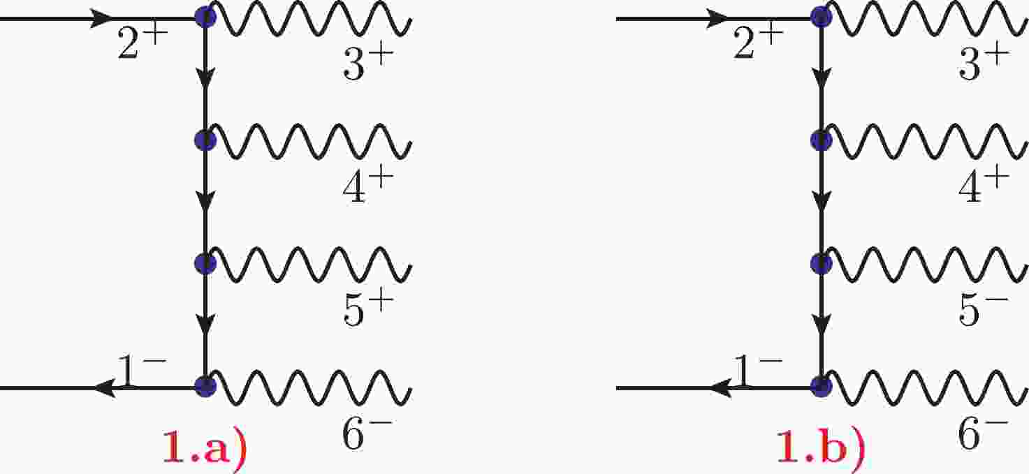
$ 0 \to e^- e^+ \gamma \gamma \gamma \gamma $ include 24 Feynman diagrams, and there are only two types of independent helicity amplitudes: one is the MHV, and the other is the NMHV. In Fig. 1, two Feynman diagrams for each of these two types of amplitudes are presented.
Figure 1. Two non-vanishing Feynman diagrams of
$0 \to e^-(1) $ $ e^+(2) \gamma(3) \gamma(4) \gamma(5) \gamma(6)$ .The MHV amplitude can be computed using the Feynman diagram method. In the BG gauge [23], the spinors of a photon can be expressed as
$ \begin{eqnarray} \epsilon^-(i) = \frac{|i\rangle [q_i|}{[i{q_i}]}\,\,, \epsilon^+(i) = \frac{|q_i \rangle [i|}{\left\langle {{q_i}i} \right\rangle }\,, \end{eqnarray} $

(9) where the momentum
$ q_i $ denotes the reference momentum. By choosing the reference momenta as$ q_6 =2 $ and$q_3=q_4= q_5=1$ and computing six nonvanishing Feynman diagrams, as shown in Fig. 1.a) (where diagrams with all permutations of (3, 4, 5) should be summed), we find that the MHV amplitudes can be expressed as$ \begin{eqnarray} A^{{{{\rm{tree}}}}}_6(1_e^-,2_{\bar{e}}^+,3_{\gamma}^+,4_{\gamma}^+,5_{\gamma}^+, 6_{\gamma}^-) = Q_e^4\frac{{\left\langle {12} \right\rangle }^2 {\left\langle {16} \right\rangle }^2}{\left\langle {13} \right\rangle \left\langle {23} \right\rangle \left\langle {14} \right\rangle \left\langle {24} \right\rangle \left\langle {15} \right\rangle \left\langle {25} \right\rangle }\,. \end{eqnarray} $

(10) Clearly, the amplitude is invariant under the exchange
$ 3 \leftrightarrow 4 $ , or$ 4 \leftrightarrow 5 $ , or$ 5 \leftrightarrow 3 $ , which is expected owing to the bosonic nature of photons. Such an amplitude can also be obtained using the BCFW method and taking the$ [1, 2 \rangle $ shift. Then, utilizing boson exchange symmetry, we arrive at the amplitude$ \begin{aligned}[b]& \frac{\left\langle {16} \right\rangle ^2 }{\left\langle {23} \right\rangle \left\langle {24} \right\rangle \left\langle {25} \right\rangle } \Bigg \{ \frac{\left\langle {23} \right\rangle ^2}{\left\langle {13} \right\rangle \left\langle {43} \right\rangle \left\langle {53} \right\rangle } + \frac{\left\langle {24} \right\rangle ^2}{\left\langle {14} \right\rangle \left\langle {34} \right\rangle \left\langle {54} \right\rangle }\\& + \frac{\left\langle {25} \right\rangle ^2}{\left\langle {15} \right\rangle \left\langle {35} \right\rangle \left\langle {45} \right\rangle } \Bigg \}\,. \end{aligned} $

(11) After combining all terms in the brackets, it is found that
$ \begin{aligned}[b]& \frac{\left\langle {23} \right\rangle ^2}{\left\langle {13} \right\rangle \left\langle {43} \right\rangle \left\langle {53} \right\rangle } + \frac{\left\langle {24} \right\rangle ^2}{\left\langle {14} \right\rangle \left\langle {34} \right\rangle \left\langle {54} \right\rangle } + \frac{\left\langle {25} \right\rangle ^2}{\left\langle {15} \right\rangle \left\langle {35} \right\rangle \left\langle {45} \right\rangle } \\=& \frac{\left\langle {12} \right\rangle ^2}{\left\langle {13} \right\rangle \left\langle {14} \right\rangle \left\langle {15} \right\rangle }\,. \end{aligned} $

(12) We then arrive at the result given in Eq. (10) from Eq. (11). The MHV helicity amplitudes with more photons of the process
$ 0 \to e^-(1^-) e^+(2^+) \gamma^-(3^-) \gamma^+(4^+) \cdots \gamma^+(n^+) $ can be assumed as$ \begin{aligned}[b]& A^{{{{\rm{tree}}}}}_{n}(1_e^-,2_{\bar{e}}^+,3_{\gamma}^-,4_{\gamma}^+,5_{\gamma}^+, 6_{\gamma}^+, \cdots, n_{\gamma}^+)\\& \rightarrow A^{{{{\rm{tree}}}}}_4(1_e^-,2_{\bar{e}}^+,3_{\gamma}^-,4_{\gamma}^+) \frac{\left\langle {12} \right\rangle }{\left\langle {15} \right\rangle \left\langle {25} \right\rangle } \cdots \frac{\left\langle {12} \right\rangle }{\left\langle {1n} \right\rangle \left\langle {2n} \right\rangle }\,, \end{aligned} $

(13) which have the correct mass dimensions, the correct helicity index for each spinor, and boson exchange symmetries among indices (
$ 4, 5, \cdots, $ and n).Using the BCFW method and taking the shift
$ [1, 2 \rangle $ , we can obtain the amplitude in the following form:$ \begin{aligned}[b]&\frac{\langle 13\rangle^{2}}{\langle 24\rangle \cdots\langle 2 n\rangle}\Bigg\{\frac{\langle 24\rangle^{n-4}}{\langle 14\rangle\langle 54\rangle\langle 64\rangle \cdots\langle n 4\rangle}+\cdots\\&+\frac{\langle 2 n\rangle^{n-4}}{\langle 1 n\rangle\langle 4 n\rangle\langle 5 n\rangle \cdots\langle(n-1) n\rangle}\Bigg\}, \end{aligned} $

(14) which maintains the boson exchanging symmetries. Using induction, we can arrive at the result given in Eq. (13) from Eq. (14). Therefore, the MHV amplitudes of QED can be elegantly expressed as
$ \begin{aligned}[b]& A^{{{{\rm{tree}}}}}_{n}(1_e^-,2_{\bar{e}}^+,3_{\gamma}^-,4_{\gamma}^+,5_{\gamma}^+, 6_{\gamma}^+, \cdots, n_{\gamma}^+) \\=& Q_e^{n-2} \frac{{\left\langle {13} \right\rangle }^2 {\left\langle {12} \right\rangle }^{n-4}}{\left\langle {14} \right\rangle \left\langle {24} \right\rangle \left\langle {15} \right\rangle \left\langle {25} \right\rangle \cdots \left\langle {1n} \right\rangle \left\langle {2n} \right\rangle }\,, \end{aligned} $

(15) which has only one term and was obtained in [23].
The NMHV amplitude can be computed using the Feynman diagram method in the BG gauge. By choosing the gauge with
$ q_3 = q_4 =1 $ and$ q_5 = q_6 = 2 $ and computing eight non-vanishing Feynman diagrams, we arrive at the amplitude of the NMHV, which can be expressed as$ \begin{aligned}[b]& A^{{{{\rm{tree}}}}}_6(1_e^-,2_{\bar{e}}^+,3_{\gamma}^+,4_{\gamma}^+,5_{\gamma}^-, 6_{\gamma}^-)\\ =&Q_e^4 \left \{ \frac{1 }{\left\langle {13} \right\rangle \left\langle {23} \right\rangle \left\langle {14} \right\rangle \left\langle {24} \right\rangle [15] [25] [16] [26] } S^1_6 + S^2_6 \right \} \,, \end{aligned} $

(16) where the term
$ S_6^1 $ is computed from the four Feynman diagrams given in Fig. 2, as follows: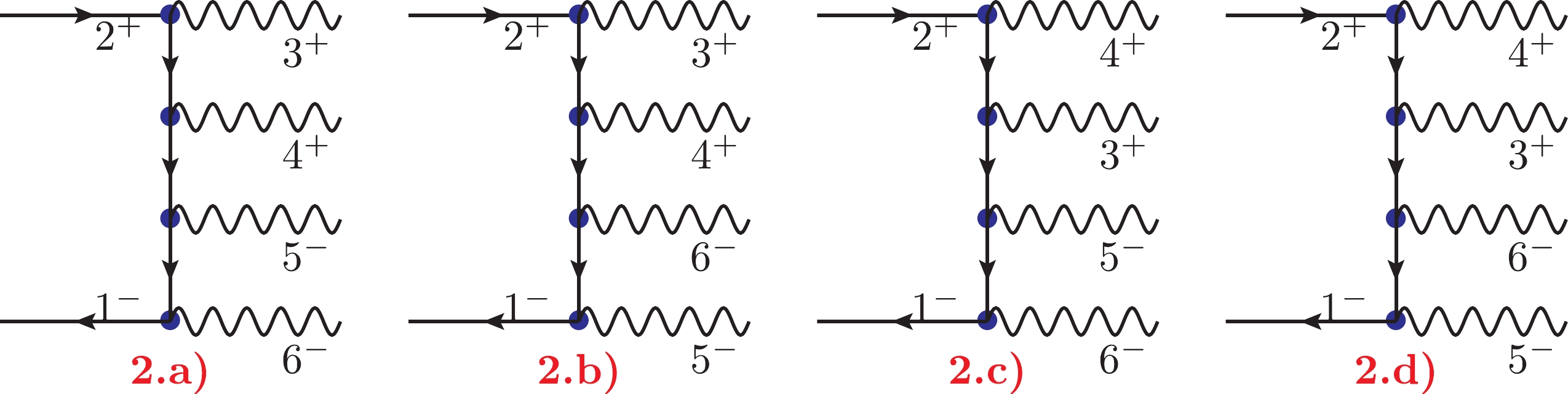
Figure 2. Four Feynman diagrams contributing to the term
$ S^1_6 $ .$ \begin{eqnarray} S_6^1 = \left\langle {12} \right\rangle [12] \,\, \langle 1 | \not k_{156} |2] \,\, S_{156} = \left\langle {12} \right\rangle [12] \,\, \langle 1 | 5+6 |2] \,\, S_{156} \,, \end{eqnarray} $

(17) When we consider the soft limits, it is noted that the following two relations are crucial:
$ \begin{eqnarray} \langle 1 | {\not k} _{156} |2] = - \langle 1 | {\not k}_{234} |2] \end{eqnarray} $

(18) and
$ \begin{eqnarray} S_{234} = S_{156} = (k_2 + k_3 + k_4)^2 = (k_1 + k_5 + k_6)^2\,, \end{eqnarray} $

(19) which are the direct results of momentum conservation
$ k_1 +k_2 +k_3 +k_4 +k_5+k_6=0 $ . These two relations are also helpful for understanding the symmetric features of$ S^1_6 $ . Clearly,$ S^1_6 $ is invariant under the exchange transformations$ 3 \leftrightarrow 4 $ and$ 5 \leftrightarrow 6 $ .The term
$ S_6^2 $ can be expressed in symmetric form from the four Feynman diagrams given in Fig. 3 as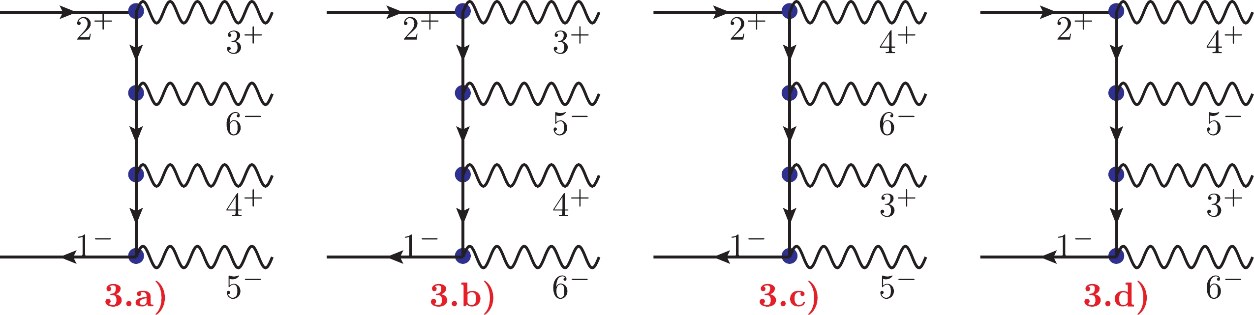
Figure 3. Four non-vanishing Feynman diagrams contributing to the term
$ S^2_6 $ .$ \begin{aligned}[b] S_6^2 = &\frac{1}{ \left\langle {14} \right\rangle [26]} \frac{ \left\langle {15} \right\rangle [23]}{[15] \left\langle {23} \right\rangle } \frac{\langle 6 |{\not k}_{236} | 4 ] }{S_{236}} \\&+ \frac{1}{ \left\langle {14} \right\rangle [25]} \frac{ \left\langle {16} \right\rangle [23]}{[16] \left\langle {23} \right\rangle } \frac{ \langle 5 |{\not k}_{235} | 4 ] }{S_{235}} \\ & + \frac{1}{ \left\langle {13} \right\rangle [26]} \frac{ \left\langle {15} \right\rangle [24]}{[15] \left\langle {24} \right\rangle } \frac{ \langle 6 |{\not k}_{246} | 3 ] }{S_{246}} \\&+ \frac{1}{ \left\langle {13} \right\rangle [25]} \frac{ \left\langle {16} \right\rangle [24]}{[16] \left\langle {24} \right\rangle } \frac{ \langle 5 |{\not k}_{245} | 3 ] }{S_{245}}\,. \end{aligned} $

(20) Using the fact that
$ \langle i | i+j+k | j]=\langle i |k | j] $ , we can present the term$ S_6^2 $ as$ \begin{aligned}[b] S_6^2 = &\frac{1}{ \left\langle {14} \right\rangle [26]} \frac{ \left\langle {15} \right\rangle [23]}{[15] \left\langle {23} \right\rangle } \frac{\langle 6 |2+3 | 4 ] }{S_{236}} \\&+ \frac{1}{ \left\langle {14} \right\rangle [25]} \frac{ \left\langle {16} \right\rangle [23]}{[16] \left\langle {23} \right\rangle } \frac{ \langle 5 |2+3| 4 ] }{S_{235}} \\ & + \frac{1}{ \left\langle {13} \right\rangle [26]} \frac{ \left\langle {15} \right\rangle [24]}{[15] \left\langle {24} \right\rangle } \frac{ \langle 6 |2+4 | 3 ] }{S_{246}} \\&+ \frac{1}{ \left\langle {13} \right\rangle [25]} \frac{ \left\langle {16} \right\rangle [24]}{[16] \left\langle {24} \right\rangle } \frac{ \langle 5 |2+4 | 3 ] }{S_{245}}\, \end{aligned} $

(21) $ \quad = [P(5,6)] [P(3,4)] \frac{1}{ \left\langle {14} \right\rangle [26]} \frac{ \left\langle {15} \right\rangle [23]}{[15] \left\langle {23} \right\rangle } \frac{\langle 6 |2+3 | 4 ] }{S_{236}} \,, $

(22) where we have use the permutation group symbols
$ [P(5,6)] $ and$ [P(3,4)] $ to simplify the results.$ [P(i,j)] $ denotes the sum of all group elements of the permutation group of two objects, i.e.,$ [P(i,j)] = E + P(i,j) $ . Because photons$ 5 $ and$ 6 $ ($ 3 $ and$ 4 $ ) have the same helicity, there are boson exchange symmetries.In total, the amplitude given in Eq. (16) is manifestly invariant under the exchanges
$ 3 \leftrightarrow 4 $ and$ 5 \leftrightarrow 6 $ , as required by boson exchange symmetry. We note that$ S^2_6 $ vanishes when any one of the photons moves toward its soft limit. With this property, the form given in Eq. (16) has good features when considering all soft and collinear limits.It should be noted that although a general form of the amplitudes with an arbitrary number of photons was formulated in terms of Feynman diagrams in reference [25], the number of terms increases with
$ n! $ (n is the number of photons). In contrast, in the BG gauge, there is only one compact term for the MHV amplitudes, as shown above. Although there is no general form of the NMHV and N$ ^2 $ MHV (or higher) amplitudes for more photons in the BG gauge, the actual forms of the NMHV or higher order amplitudes are dependent on the helicity sequences (or spin chain of photons). Once the helicity sequences are specified, it it straightforward to express the amplitudes in terms of spinor brackets and permutation groups. Below, we present the amplitudes of$ 0 \to e^- e^+ 5 \gamma $ and$ 0 \to e^- e^+ 6\gamma $ for later reference.To realize boson exchange symmetry, in the total amplitude, all possible permutations of photons with the same helicities must be considered. For these helicity configurations, both end particles, denoted as
$ \bar{f}(2^+) $ and$ f(1^-) $ , are fixed, and the helicities of photons adjoined with fermion particles are also fixed in the BG gauge. These facts constrain all allowed helicity configurations. For the NMHV 6-point amplitude, there are only two helicity configurations, i.e.,$ +++--- $ and$++-+--$ . For the NMHV 7-point amplitude, there are only three allowed helicity configurations, i.e.,$ ++++--- $ ,$+++-+--$ , and$++-++--$ . Moreover, for the NMHV 8-point amplitude, there are only four allowed helicity configurations, i.e.,$ +++++--- $ ,$++++-+--$ ,$+++-++--$ , and$++-+++--$ . For the N$ ^2 $ MHV of the 8-point amplitude, there are only six allowed helicity configurations, i.e.,$ ++++---- $ ,$ +++-+--- $ ,$ ++-++--- $ ,$+++--+--$ ,$++-+--+--$ , and$++--++--$ . For more general amplitudes of the process$ 0\to e^- e^+ \gamma_1^+ \cdots \gamma_n^+ \gamma_1^- \cdots \gamma_m^- $ with$ m \leq n $ , the number of allowed helicity configurations is given as$ \begin{eqnarray} N_S = \frac{(m+n-2)!}{(m-1)! \,\,(n-1)! }\,, \end{eqnarray} $

(23) which is significantly less than the number of amplitudes constructed directly from Feynman diagrams (which should be counted as
$ (m+n)! $ ).It is noteworthy that terms calculated in the helicity amplitude can be combined into a form with fewer terms; for example, there is only one term for the MHV amplitudes. For helicity amplitudes beyond the MHVA, a smaller number of terms can be achieved, similar to the helicity amplitudes given in Eq. (25), Eq. (30), and Eq. (35). In contrast, if we construct the amplitude directly from Feynman diagrams, there are n! terms, regardless of the helicity structure assumed.
Subsequently, the NMHV amplitude
$ A^{{{{\rm{tree}}}}}_7(1_e^-,2_{\bar{e}}^+, 3_{\gamma}^+,4_{\gamma}^+, 5_{\gamma}^+, 6_{\gamma}^-, 7_{\gamma}^-) $ can be efficiently computed using the off-shell amplitude method in the BG gauge. Using the Feynman diagrams given in Fig. 4 as examples and the boson exchange symmetries of photons that have the same helicities, we can obtain the total amplitude. In terms of helicity configurations, the total amplitude can be organized into the following form: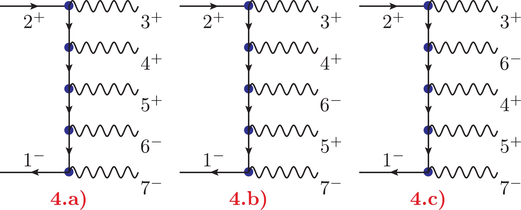
Figure 4. Three types of non-vanishing Feynman diagrams contributing to the term
$ A^{{{{\rm{tree}}}}}_7 $ .$ A^{{{{\rm{tree}}}}}_7(1_e^-,2_{\bar{e}}^+,3_{\gamma}^+,4_{\gamma}^+,5_{\gamma}^+, 6_{\gamma}^-, 7_{\gamma}^-)= Q_e^5 \left \{ S^1_7 + S^2_7 + S_7^3 \right \} \,, $

(24) where each
$ S^i_7 $ term is given below.$ \begin{eqnarray} S^1_7 &= & \frac{\left\langle {12} \right\rangle ^2 [12] \,\, \langle 1 | 6 + 7 |2] \,\, S_{167} }{\prod_{i=3,4,5} \left\langle {1 i} \right\rangle \left\langle {2 i} \right\rangle \prod_{j=6,7} [1j] [2j] }\,, \end{eqnarray} $

(25) $ \begin{aligned}[b] S^2_7 = &\frac{\left\langle {12} \right\rangle }{\prod_{i=3,4,5}\left\langle {1i} \right\rangle } [P(6,7)] \Bigg [ \frac{\left\langle {17} \right\rangle }{[17] [26]}[P(34,5)] \\&\times \frac{ \langle 1 | 3+4| 2 ] }{ \left\langle {23} \right\rangle \left\langle {24} \right\rangle } \frac{[5 | 1 + 7 | 6 \rangle}{S_{157}} \Bigg ] \,, \end{aligned} $

(26) $ \begin{aligned}[b] S^3_7=& [P(6,7)] \frac{\left\langle {17} \right\rangle ^2}{[17] [26] } \Bigg [ [P(3,45)] \\&\times \frac{[23]}{\left\langle {23} \right\rangle } \frac{1}{\left\langle {14} \right\rangle \left\langle {15} \right\rangle S_{236}} [P(4,5)] \frac{[5]7 [4 | 2 + 3 | 6 \rangle}{S_{157}} \Bigg ] \,, \end{aligned} $

(27) where
$ S_7^1 $ includes the contribution of diagrams with the helicity configuration$ ++++--- $ , as given in Fig. 4.a),$ S^2_7 $ includes the contribution of diagrams with the helicity configuration$+++-+--$ , as given in Fig. 4.b), and$ S^3_7 $ includes the contribution of diagrams with the helicity configuration$++-++--$ , as shown in Fig. 4.c). The symbol$ [P(34,5)] $ denotes the sum of the subset of the permutation group$ E + P_{35} + P_{45} $ , because the symmetry between$ 3 $ and$ 4 $ is realized, and only the symmetry with$ 5 $ must be restored, as shown in Fig. 4.b). The symbol$ [P(34,5)] $ acts to the terms in the right hand side, i.e., after the action, the terms will be changed to the sum of three terms. For example,$ \begin{aligned}[b]& [P(34,5)] \frac{ \langle 1 | 3+4| 2 ] }{ \left\langle {23} \right\rangle \left\langle {24} \right\rangle } \frac{[5 | 1 + 7 | 6 \rangle}{S_{157}} \\=& \frac{ \langle 1 | 3+4| 2 ] }{ \left\langle {23} \right\rangle \left\langle {24} \right\rangle } \frac{[5 | 1 + 7 | 6 \rangle}{S_{157}} + \frac{ \langle 1 | 4+5| 2 ] }{ \left\langle {24} \right\rangle \left\langle {25} \right\rangle } \frac{[3 | 1 + 7 | 6 \rangle}{S_{137}}\\& + \frac{ \langle 1 | 3+5| 2 ] }{ \left\langle {23} \right\rangle \left\langle {25} \right\rangle } \frac{[4 | 1 + 7 | 6 \rangle}{S_{147}} \,. \end{aligned} $

(28) Similarly, the symbol
$ [P(3,45)] $ denotes the sum of$ E + P_{34} + P_{35} $ . When$ [P(3,45)] [P(4,5)] $ , we arrive at$ [P(3,45)] [P(4,5)] = [P(3,4,5)] $ , which denotes the sum of all allowed permutations of three objects, i.e.,$ [P(3,4,5)] = E + P_{34} + P_{35}+ P_{45} + P_{345} + P_{345}^2 $ .To realize boson exchange symmetry, we use permutation group symbols. For example, in
$ S^2_7 $ ,$ [P(6,7)] $ indicates that two terms should be added. In$ S^3_7 $ ,$[P(4,5)] \frac{[47] [5 | 2+3| 6\rangle}{S_{147}}$ means$\frac{[57] [4 | 2+3| 6\rangle}{S_{157}} + \frac{[47] [5 | 2+3| 6\rangle}{S_{147}}$ . It is clear that the boson exchange symmetries among photons with the same helicities for$ A^{{{{\rm{tree}}}}}_7 $ are explicit.Similarly, the NMHV amplitude
$A^{{{{\rm{tree}}}}}_8(1_e^-,2_{\bar{e}}^+, 3_{\gamma}^+,4_{\gamma}^+,5_{\gamma}^+, 6_{\gamma}^+, 7_{\gamma}^-,8_\gamma^-)$ can be efficiently computed using the off-shell amplitude method. We can use the Feynman diagrams given in Fig. 5 as a guide to compute the results of each helicity configuration using the off-shell amplitudes and permutation symmetries. The results are organized into the following four helicity configurations:$+ ++++-- -$ (denoted as$ S^1_{8N} $ ),$ + +++-+- - $ (denoted as$ S^2_{8N} $ ),$ + ++-++- - $ (denoted as$ S^3_{8N} $ ), and$ + +-+++- - $ (denoted as$ S^4_{8N} $ ). The total amplitude can be organized into the following form: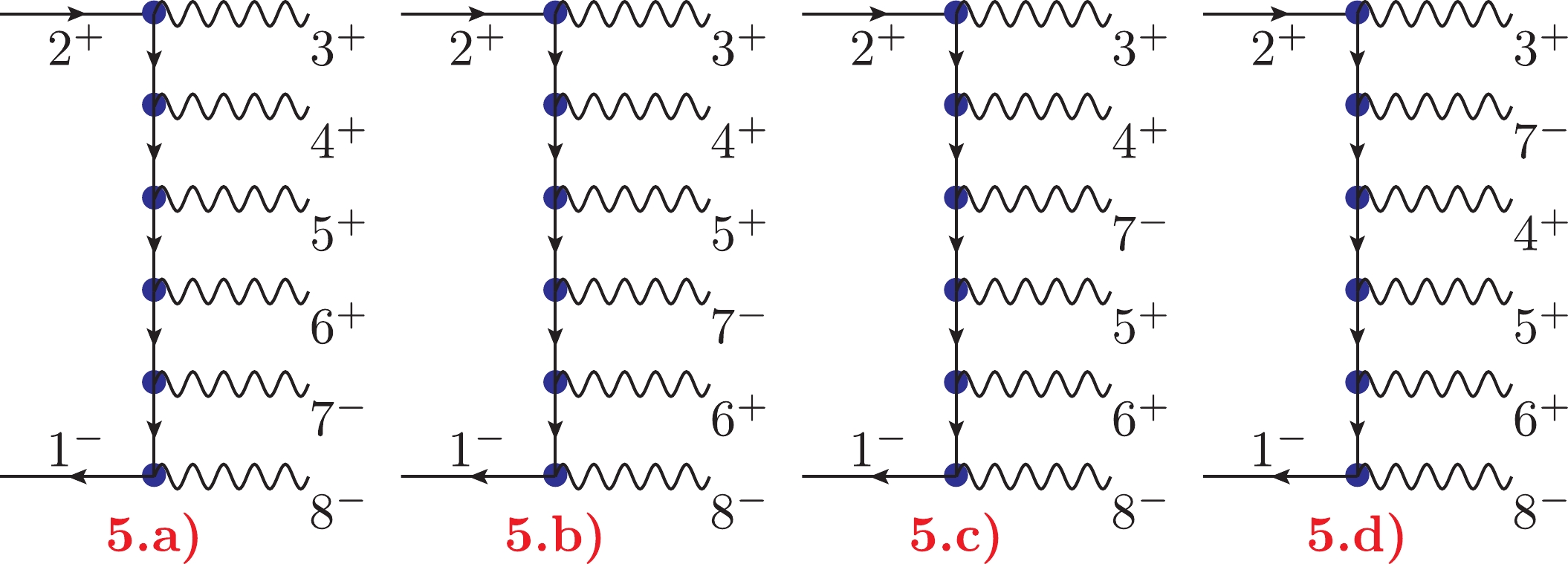
Figure 5. Four types of non-vanishing Feynman diagrams contributing to the term
$ A^{{{{\rm{tree}}}}}_8 $ .$ \begin{aligned}[b]& A^{{{{\rm{tree}}}}}_{8N}(1_e^-,2_{\bar{e}}^+,3_{\gamma}^+,4_{\gamma}^+,5_{\gamma}^+, 6_{\gamma}^+, 7_{\gamma}^-, 8_\gamma^-) \\=& Q_e^6 \left \{ S^1_{8N} + S^2_{8N} + S_{8N}^3 + S_{8N}^4 \right \} \,, \end{aligned} $

(29) where the
$ S^i_8 $ term corresponding to each figure in Fig. 5 is given as$ \begin{eqnarray} S_{8N}^1 &=& \frac{\left\langle {12} \right\rangle ^3 [12] \,\, \langle 1 | 7 + 8 |2] \,\, S_{178} }{\prod_{i=3,4,5,6} \left\langle {1 i} \right\rangle \left\langle {2 i} \right\rangle \prod_{j=7,8} [1j] [2j ] }\,, \end{eqnarray} $

(30) $ \begin{aligned}[b] S_{8N}^2=& \frac{\left\langle {12} \right\rangle ^2 }{\prod_{i=3,4,5,6} \left\langle {1 i} \right\rangle } [P(345,6)] [P(7,8)]\\&\times \left\{ \frac{\langle 1 | 3 + 4 + 5 | 2 ] }{\prod_{j=3,4,5}\left\langle {2 j} \right\rangle } \frac{\left\langle {18} \right\rangle }{[18]} \frac{[6 | 1+8 | 7 \rangle }{[27] S_{168}} \right \}\, , \end{aligned} $

(31) $ \begin{aligned}[b] S_{8N}^3 = & \frac{\left\langle {12} \right\rangle }{\prod_{i=3,4,5,6} \left\langle {1 i} \right\rangle} [P(7,8)] \frac{\left\langle {18} \right\rangle ^2}{[27] [18] } \Bigg\{ [P(34,56)] \\ & \left. \times \frac{\langle 1 | 3+4 |2] }{\left\langle {23} \right\rangle \left\langle {24} \right\rangle S_{1568}} [P(5,6)] \frac{[86] [5 | 1 + 6+8 | 7\rangle}{S_{168}} \right\} \,, \end{aligned} $

(32) $ \begin{aligned}[b] S^4_{8N} = & \left\langle {12} \right\rangle [P(7,8)] \frac{\left\langle {18} \right\rangle ^2}{[27] [18] } \left \{ [P(34,56)] \right. \\ & \frac{1}{\left\langle {15} \right\rangle \left\langle {16} \right\rangle S_{1568} } \left ( [P(3,4)]\frac{[23]}{\left\langle {23} \right\rangle }\frac{[4 | 2 + 3 | 7 \rangle }{\left\langle {14} \right\rangle S_{237}} \right )\\& \left ( [P(5,6)] \frac{[86] [5 | 1 + 6+8 | 7\rangle}{S_{168}} \right ) \Bigg \} \,, \end{aligned} $

(33) where
$ [P(345,6)]=E + P_{36} + P_{46} + P_{56} $ , which reflects the exchange symmetry among$ 3 $ ,$ 4 $ , and$ 5 $ , and$[P(34, 56)] = E + P_{35} + P_{36} + P_{45} + P_{46} + P_{35} P_{46}$ , which expresses the exchange symmetry between$ 3 $ and$ 4 $ , and the symmetry between$ 5 $ and$ 6 $ . According to these conventions, the following relation exists:$[P(3,4,5,6)]= [P(34,56)] [P(3,4)]\times$ $ [P(5,6)]$ .The N
$ ^2 $ MHV amplitude$A^{\rm tree}_8(1_e^-,\, 2_{\bar{e}}^+,\, 3_{\gamma}^+,\, 4_{\gamma}^+,\, 5_{\gamma}^+,\, 6_{\gamma}^-$ ,$ 7_{\gamma}^-,8_\gamma^-)$ can be computed from the Feynman diagrams given in Fig. 6 and can be expressed as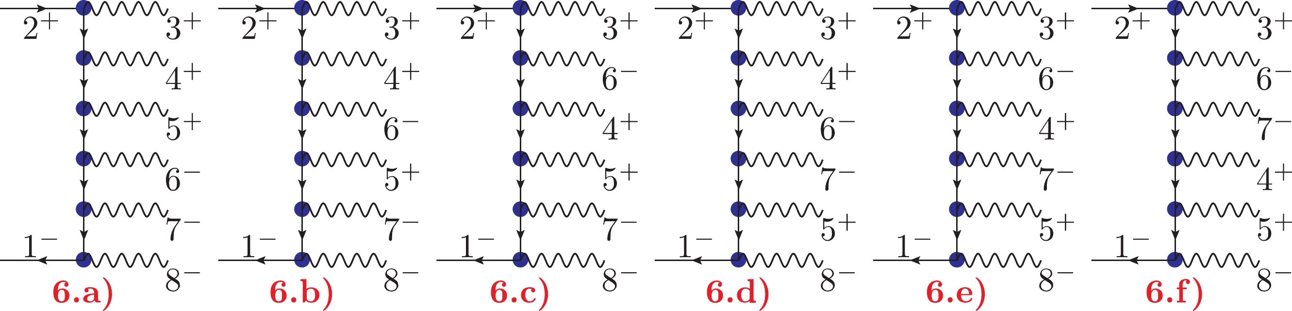
Figure 6. Six types of non-vanishing Feynman diagrams contributing to the term
$ A^{{{{\rm{tree}}}}}_8 $ .$ \begin{aligned}[b]& A^{{{{\rm{tree}}}}}_{8N^2}(1_e^-,2_{\bar{e}}^+,3_{\gamma}^+,4_{\gamma}^+,5_{\gamma}^+, 6_{\gamma}^+, 7_{\gamma}^-, 8_\gamma^-) \\=& Q_e^6 \left \{ S^1_{8N^2} + S^2_{8N^2} + S_{8N^2}^3 + S^4_{8N^2} + S^5_{8N^2} + S_{8N^2}^6 \right \} \,, \end{aligned} $

(34) where
$ S^i_{8N^2} $ corresponding to each diagram in Fig. 6 is given below.$ S^1_{8N^2} = \frac{\left\langle {12} \right\rangle ^2 [12]^2 \,\, \langle 1 | 6 + 7 + 8 |2] \,\, S_{1678} }{\prod_{i=3,4,5} \left\langle {1 i} \right\rangle \left\langle {2 i} \right\rangle \prod_{j=6,7,8} [1j] [2j] }\,, $

(35) $ \begin{aligned}[b]\\ \\ \\ \\ \\ \\ \\ \\ S^2_{8N^2} = [P(6,78)] [P(34,5)] \Bigg[ \frac{\left\langle {12} \right\rangle [12]}{(\prod_{i=3,4} \left\langle {1 i} \right\rangle \left\langle {2 i} \right\rangle) (\prod_{j=7,8}) [1j] [2j]} \frac{\langle 1 | 7+8 |2] \langle 1 | 3 + 4 \ 2] [5 | 1 + 7 + 8 | 6 \rangle}{\left\langle {15} \right\rangle [26] S_{1578}} \Bigg ]\,, \end{aligned} $

(36) $ S^3_{8N^2} =[P(34,5)] \left\{ [P(3,4)] \frac{[23]}{\left\langle {23} \right\rangle \left\langle {14} \right\rangle } \left[ [P(6,78)] \frac{[12]}{(\prod_{j=7,8} [1j] [2j])} \frac{[2 | 7+8 | 1 \rangle}{\left\langle {15} \right\rangle [26]} \frac{[4 | 2 + 3 | 6 \rangle [5 | 7 + 8| 1\rangle}{S_{236} S_{1578} } \right] \right \} \,, $

(37) $ S^4_{8N^2} = [P(6,78)]\left\{ [P(7,8)] \frac{\left\langle {18} \right\rangle }{[27] [18]} \left[ [P(34,5)] \frac{\left\langle {12} \right\rangle }{(\prod_{j=3,4} \left\langle {1 j} \right\rangle \left\langle {2 j} \right\rangle )} \frac{[2 | 3 +4 | 1 \rangle}{\left\langle {15} \right\rangle [26]} \frac{[5 | 1+8 | 7 \rangle [2 | 3+4| 6\rangle}{S_{158} S_{1578} } \right ] \right\} \,, $

(38) $ S^5_{8N^2} = [P(34,5)] [P(6,78)] \left \{ \frac{1}{\left\langle {15} \right\rangle [26]} \left [ [P(7,8)] [P(3,4)] \left( \frac{[23]}{\left\langle {23} \right\rangle \left\langle {14} \right\rangle } \frac{\left\langle {18} \right\rangle }{[27] [18]} \frac{[4 | 2+3| 6 \rangle [5 | 1 + 8| 7 \rangle [2| 5 + 7 + 8 | 1 \rangle}{S_{236} S_{158} S_{1578} } \right) \right ] \right \} \,, $

(39) $ S^6_{8N^2} = [P(3,45)] [P(67,8)] \left \{ \frac{[23]^2 \left\langle {18} \right\rangle ^2}{\left\langle {23} \right\rangle \left\langle {14} \right\rangle \left\langle {15} \right\rangle [26] [27] [18] S_{1458} } \left( [P(4,5)] [P(6,7)] \frac{\left\langle {36} \right\rangle [58] [4 | 2 + 3 + 6 | 7 \rangle}{S_{158} S_{236} } \right) \right \} \,. $

(40) It should be noted that, by using the off-shell current method given in [23] and the permutation group for boson exchange symmetry, we can express the amplitudes of a given helicity configuration in an elegant form with a smaller number of terms than that in the direct Feynman diagram method. This analytic form of amplitudes is helpful to understand the properties all shifts in the BCFW method.
-
To compute the amplitudes of the process
$ 0 \to e^- e^+ 4\gamma $ using the BCFW method, we can organize the diagrams with three types of topologies, i.e.,$ 3 \otimes 5 $ (denoted as P diagrams, as shown in Fig. 7, where$ 3 $ indicates that the left side has 3-point amplitudes and the right side has 5-point amplitudes),$ 4 \otimes 4 $ (denoted as R diagrams, as shown in Fig. 8, where both the left and right sides have 4-point amplitudes), and$ 5 \otimes 3 $ (denoted as Q diagrams, as shown in Fig. 9, where the left side has 5-point amplitudes and the right side has 3-point amplitudes). Because the shift$ [1,2\rangle $ is a natural choice to factorize the total amplitude owing to the charge conservation law, and there are 12 diagrams in total. Below, we describe all of these diagrams in detail. The diagrams for other shifts are simply subsets of these 12 diagrams.
Figure 7. Four diagrams for the
$ 3\otimes 5 $ topology are shown in the$ [1, 2 \rangle $ shift.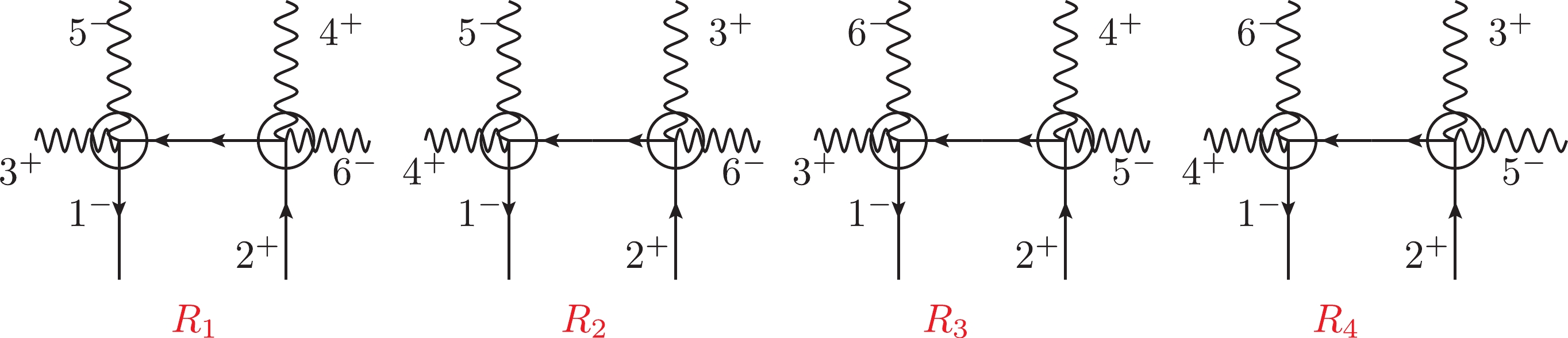
Figure 8. Four diagrams for the
$ 4\otimes 4 $ topology are shown in the$ [1, 2 \rangle $ shift.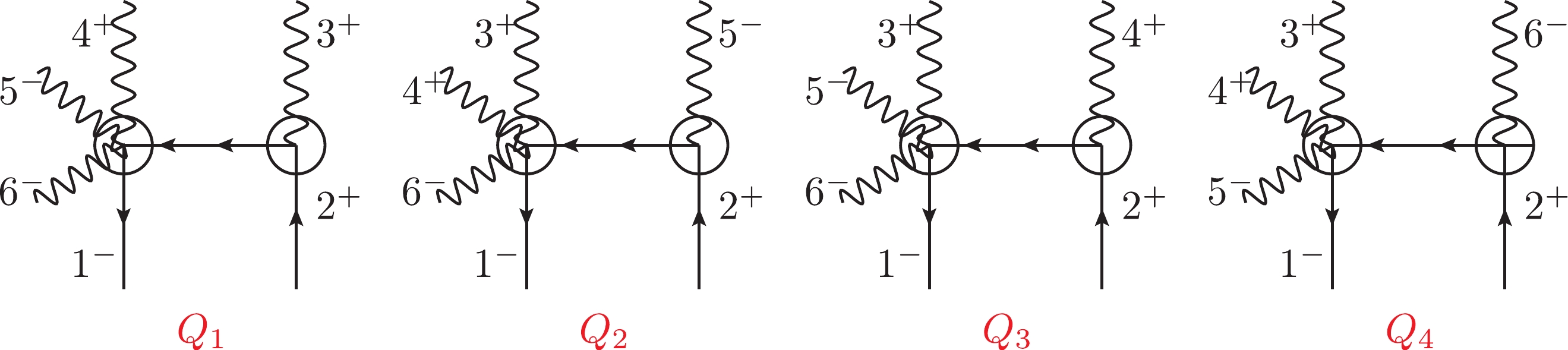
Figure 9. Four diagrams for the
$ 5\otimes 3 $ topology are shown in the$ [1, 2 \rangle $ shift.The topology
$ 3 \otimes 5 $ includes the four diagrams given in Fig. 7, labeled as$ P_1 $ ,$ P_2 $ ,$ P_3 $ , and$ P_4 $ . In these four diagrams, there is an exchange symmetry between$ P_1 $ and$ P_3 $ with$ 3 \leftrightarrow 4 $ and between$ P_2 $ and$ P_4 $ with$ 5 \leftrightarrow 6 $ . Such exchange symmetries can be used to simplify the calculation procedure. The momenta of the internal lines are denoted as$ P_1 $ ,$ P_2 $ ,$ P_3 $ , and$ P_4 $ , respectively. For example,$ P_1= \hat{k}_1 + k_3 = - (\hat{k}_2 + k_4 + k_5 + k_6) $ . The arrows in the fermion lines denote the direction of particle flow.The topology
$ 4 \otimes 4 $ includes the four diagrams given in Fig. 8, labeled as$ R_1 $ ,$ R_2 $ ,$ R_3 $ , and$ R_4 $ . In these four diagrams, there is an exchange symmetry between$ R_1 $ and$ R_2 $ with$ 3 \leftrightarrow 4 $ and between$ R_1 $ and$ R_3 $ with$ 5 \leftrightarrow 6 $ . Such exchange symmetries can be used to simplify the calculation procedure. The momenta of the internal lines are denoted as$ R_1 $ ,$ R_2 $ ,$ R_3 $ , and$ R_4 $ , respectively. For example,$ R_1= \hat{k}_1 + k_3 + k_5 = - ({\hat k}_2 + k_4 + k_6) $ .The topology
$ 5 \otimes 3 $ includes the four diagrams given in Fig. 9, labeled as$ Q_1 $ ,$ Q_2 $ ,$ Q_3 $ , and$ Q_4 $ . In these four diagrams, there is an exchange symmetry between$ Q_1 $ and$ Q_3 $ with$ 3 \leftrightarrow 4 $ and between$ Q_2 $ and$ Q_4 $ with$ 5 \leftrightarrow 6 $ . Such exchange symmetries can be used to simplify the calculation procedure. The momenta of the internal lines are denoted as$ Q_1 $ ,$ Q_2 $ ,$ Q_3 $ , and$ Q_4 $ , respectively. For example,$ Q_1=\hat{k}_2 + k_3 = - (\hat{k}_1 + k_4 + k_5 + k_6) $ .For the NMHV amplitude of the process
$ 0 \to e^-(1^-) e^+(2^+) \gamma^+(3^+) \gamma^+(4^+) \gamma^-(5^-) \gamma^-(6^-) $ , there are 30 shifts that can be defined. From the result given in Eq. (16) and in terms of the highest z power in the limit$ z \to \infty $ , they can be divided into five categories:● 1)
$ z^2 $ :$ [3, 5\rangle $ ($ [4, 5\rangle $ ) and$ [3, 6\rangle $ ($ [4, 6\rangle $ );● 2)
$ z^1 $ :$ [3, 1\rangle $ ($ [4, 1\rangle $ ) and$ [2, 5\rangle $ ($ [2, 6\rangle $ );● 3)
$ z^0 $ :$ [2,1\rangle $ ,$ [1,5\rangle $ ($ [1,6\rangle $ ), and$ [3,2\rangle $ ($ [4,2\rangle $ );● 4)
$ z^{-1} $ :$ [1, 3\rangle $ ($ [1, 4\rangle $ ),$ [5, 2\rangle $ ($ [6, 2\rangle $ ),$ [5, 1\rangle $ ($ [6, 1\rangle $ ),$ [5, 6\rangle $ ($ [6,5\rangle $ ),$ [3, 4\rangle $ ($ [4, 3\rangle $ ),$ [2, 3\rangle $ ($ [2, 4\rangle $ );● 5)
$ z^{-2} $ :$ [1, 2 \rangle $ ,$ [5,3\rangle $ ($ [6,3\rangle $ ) and$ [5,4\rangle $ ($ [6,4\rangle $ ).In Table 1, we show the power index of z in the limit
$ z \to \infty $ for all shifts. We describe shifts with$ k < 0 $ as good shifts because the boundary terms vanish and the BCFW method is expected to work. Conversely, for shifts with$ k\ge0 $ , in general, it is not expected to work.shifts $ [i, j\rangle (i<j) $ 

$ [1, 2\rangle $ 

$ [1, 3\rangle $ 

$ [1, 4 \rangle $ 

$ [1, 5\rangle $ 

$ [1, 6\rangle $ 

k −2 −2 −2 0 0 shifts $ [i, j\rangle (i<j) $ 

$ [2, 3 \rangle $ 

$ [2, 4\rangle $ 

$ [2, 5\rangle $ 

$ [2, 6 \rangle $ 

$ [3, 4\rangle $ 

k −1 −1 1 1 −1 shifts $ [i, j\rangle (i<j) $ 

$ [3, 5\rangle $ 

$ [3, 6 \rangle $ 

$ [4, 5\rangle $ 

$ [4, 6\rangle $ 

$ [5, 6 \rangle $ 

k 2 2 2 2 −1 shifts $ [i, j\rangle (i> j) $ 

$ [2, 1\rangle $ 

$ [3,1\rangle $ 

$ [4, 1 \rangle $ 

$ [5, 1\rangle $ 

$ [6, 1\rangle $ 

k 0 2 2 −1 −1 shifts $ [i, j\rangle (i> j) $ 

$ [3, 2 \rangle $ 

$ [4,2 \rangle $ 

$ [5,2\rangle $ 

$ [6, 2 \rangle $ 

$ [4, 3\rangle $ 

k 0 0 −2 −2 −1 shifts $ [i, j\rangle (i> j) $ 

$ [5, 3\rangle $ 

$ [6, 3 \rangle $ 

$ [5, 4\rangle $ 

$ [6, 4\rangle $ 

$ [6, 5 \rangle $ 

k −2 −2 −2 −2 −1 Table 1. Leading
$ z^k $ in the limit$ z \to \infty $ of shifts$ [i, j\rangle $ in the BCFW method for$ 0 \to e^-(1^-) e^+(2^+) \gamma(3^+) \gamma(4^+) \gamma(5^-) \gamma(6^-) $ .Here, we demonstrate the results of the shift
$ [1, 2 \rangle $ , which has a vanishing boundary term. In the shift$ [1, 2 \rangle $ , there are three independent terms that must be computed, while the rest can be obtained from the boson exchange symmetries of photons. The total amplitude can be computed as$ A_{t} = A_P^{12} + A_Q^{12} + A_R^{12}\,, $

(41) $ A_{P_1}^{12} = A_{P_3}^{12} = A_{Q_2}^{12} = A_{Q_4}^{12}=0 \,, $

(42) $ A_{P_2}^{12} = \frac{S_{125}[25]\langle6|1+5|2]^2}{[15] \langle3|1+5|2] \langle3|1+2|5] \langle4|1+5|2] \langle4|1+2|5]} \,, $

(43) $ A_{P_4}^{12} = \frac{S_{126}[26]\langle5|1+6|2]^2}{[16] \langle3|1+6|2] \langle3|1+2|6] \langle4|1+6|2] \langle4|1+2|6]} \,, $

(44) $ A_{Q_1}^{12} = (-)\frac{ S_{123}\langle13\rangle \langle1|2+3|4]^2 }{ \langle23\rangle \langle3|1+2|5] \langle1|2+3|5] \langle3|1+2|6] \langle1|2+3|6] } \,, $

(45) $ A_{Q_3}^{12} = (-)\frac{ S_{124} \langle14\rangle \langle1|2+4|3]^2}{ \langle24\rangle \langle4|1+2|5] \langle1|2+4|5] \langle4|1+2|6] \langle1|2+4|6] } \,, $

(46) $ A_{R_1}^{12} = (-)\frac{\langle15\rangle^2[24]^2 \langle1|3+5|2] }{S_{135}\langle13\rangle[26]\langle1|3+5|6] \langle3|1+5|2]} \,, $

(47) $ A_{R_2}^{12} = (-)\frac{\langle15\rangle^2 [23]^2 \langle1|4+5|2] }{S_{145}\langle14\rangle [26] \langle1|4+5|6] \langle4|1+5|2] } \,, $

(48) $ A_{R_3}^{12} = (-) \frac{\langle16\rangle^2 [24]^2 \langle1|3+6|2] }{S_{136}\langle13\rangle [25] \langle1|3+6|5] \langle3|1+6|2] } \,, $

(49) $ A_{R_4}^{12} = (-)\frac{\langle16\rangle^2 [23]^2 \langle1|4+6|2] }{S_{146}\langle14\rangle [25] \langle1|4+6|5] \langle4|1+6|2] } \,. $

(50) We compute the amplitudes of all shifts for the process
$ 0 \to e^- e^+ 4 \gamma $ . We find that the obtained amplitudes have very different forms. Because it is difficult to demonstrate the equivalence of the results given in Eq. (16) and those obtained using BCFW shifts, we resort to numerical methods to examine whether they are equivalent. We consider all allowed shifts in the BCFW method and examine whether they can yield the same results as those obtained from the Feynman diagram method. To conduct the numerical analysis, we use the Mathematica tool "S@M", which is a Mathematica Implementation of the Spinor-Helicity Formalism [26].The numerical results are summarized in Table 2.
shifts $ [i, j\rangle (i<j) $ 

$ [1, 2\rangle $ 

$ [1, 3\rangle $ 

$ [1, 4 \rangle $ 

$ [1, 5\rangle $ 

$ [1, 6\rangle $ 

$ \times \circ $ 

$ \times \circ $ 

shifts $ [i, j\rangle (i<j) $ 

$ [2, 3 \rangle $ 

$ [2, 4\rangle $ 

$ [2, 5\rangle $ 

$ [2, 6 \rangle $ 

$ [3, 4\rangle $ 

$ \times \times $ 

$ \times \times $ 

shifts $ [i, j\rangle (i<j) $ 

$ [3, 5\rangle $ 

$ [3, 6 \rangle $ 

$ [4, 5\rangle $ 

$ [4, 6\rangle $ 

$ [5, 6 \rangle $ 

$ \times \times $ 

$ \times \times $ 

$ \times \times $ 

$ \times \times $ 

shifts $ [i, j\rangle (i> j) $ 

$ [2, 1\rangle $ 

$ [3,1\rangle $ 

$ [4, 1 \rangle $ 

$ [5, 1\rangle $ 

$ [6, 1\rangle $ 

$ \surd \surd $ 

$ \times \times $ 

$ \times \times $ 

shifts $ [i, j\rangle (i> j) $ 

$ [3, 2 \rangle $ 

$ [4,2 \rangle $ 

$ [5,2\rangle $ 

$ [6, 2 \rangle $ 

$ [4, 3\rangle $ 

$ \times \surd $ 

$ \times \surd $ 

shifts $ [i, j\rangle (i> j) $ 

$ [5, 3\rangle $ 

$ [6, 3 \rangle $ 

$ [5, 4\rangle $ 

$ [6, 4\rangle $ 

$ [6, 5 \rangle $ 

Table 2. Results of the shifts
$ [i, j\rangle $ in the BCFW method for$ 0 \to e^-(1^-) e^+(2^+) \gamma(3^+) \gamma(4^+) \gamma(5^-) \gamma(6^-) $ .● First, shifts such as
$ [2, 5\rangle $ ,$ [2, 6\rangle $ ,$ [3, 5\rangle $ ,$ [3, 6\rangle $ ,$ [4, 5\rangle $ ,$ [4, 6\rangle $ ,$ [3,1\rangle $ , and$ [4, 1\rangle $ cannot produce the correct results without a known boundary term. The reason lies in the fact that shifts such as$ [2, 5\rangle $ ,$ [2, 6\rangle $ ,$ [3,1\rangle $ , and$ [4, 1\rangle $ change the amplitude into the form$ \begin{aligned}[b] A(z) =& C_1 \dfrac{(z^2 + a_1 z + a_2) (z+ b) (z+c) }{(z -z_1)} \\&+ C_2 \dfrac{(z+b_1) (z+c_1) (z+d_1)}{(z-z_1)(z-z_2)} \end{aligned} $

and shifts such as
$ [3, 5\rangle $ ,$ [3, 6\rangle $ ,$ [4, 5\rangle $ , and$ [4, 6\rangle $ change the amplitude into the form$ \begin{aligned}[b] A(z) = C_1 \dfrac{(z+a) (z+b) }{(z-z_1)(z-z_2)} + C_2 \dfrac{(z+a)(z+b)(z+c)}{(z-z_1)(z-z_2)} \end{aligned} $

which has either an undetermined or non-vanishing boundary value in the limit
$ \lim_{z \to \infty} \oint \dfrac{A(z)}{z} $ .● Second, among the 30 shifts of the BCFW method, there are 18 shifts that satisfy the necessary condition of the BCFW method and can produce the correct results. Generally, a shift with the inverse helicity of a pair of spinors in the amplitude can always work. For example, with both a fermion and photon in the amplitude, such as the amplitude
$ A^{{{{\rm{tree}}}}}_6(1_e^-,2_{\bar{e}}^+,3_{\gamma}^-,4_{\gamma}^-,5_{\gamma}^+, 6_{\gamma}^+) $ , shifts such as$ [5, 4\rangle $ ,$ [6, 4\rangle $ ,$ [5, 3\rangle $ , and$ [6, 3\rangle $ can always work. Similarly, this also holds for shifts such as$ [1, 3\rangle $ ,$ [1, 4\rangle $ ,$ [5, 2 \rangle $ , and$ [6, 2\rangle $ . These shifts have vanishing boundary terms.● Third, it should be noted that the shift
$ [2,1\rangle $ can produce the correct results, which is slightly surprising. It is not expected to work from our experience of 4-point and 5-point amplitudes. Why does this shift work? It is found that in this shift, the amplitude given in Eq. (16) changes to the form$ \begin{aligned}[b] A^{21}(z) =& C_1 \frac{(z^2+ a_1 z + a_2) (z + b)}{(z-z_1) (z -z_2) (z -z_3) (z -z_4)} \\&+ C_2 \frac{(z + c_1)(z + c_2)(z + c_3)}{(z - z_5) (z - z_6)(z - z_7)} \,. \end{aligned} $

(51) In the limit
$ z \to \infty $ , the first term proportional to$ C_1 $ vanishes, and the second term proportional to$ C_2 $ apparently leads to a non-vanishing boundary value. Fortunately,$ C_2 $ is found to have the following term:$ \begin{eqnarray} \frac{1}{\langle 2 | 3+6 |1 ] } + \frac{1}{\langle 2 | 3+5 | 1 ] } + \frac{1}{\langle 2 | 4+6 | 1 ] } + \frac{1}{\langle 2 | 4+5 | 1 ] } \,, \end{eqnarray} $

(52) and it can be proven that this term is vanishing when we consider that
$ \langle 2 | 3+6 | 1] = - \langle 2 | 4 + 5 | 1] $ and$ \langle 2 | 3+5 | 1] = - \langle 2 | 4 + 6 | 1] $ in terms of momentum conservation. This explains why the shift$ [2, 1 \rangle $ can work. Such cancellation only occurs at the full amplitude level, which was found in Ref. [27].● We would like to emphasize that although each shift, such as
$ [1, 5 \rangle $ ,$ [1, 6 \rangle $ ,$ [3, 2 \rangle $ , and$ [4, 2 \rangle $ , cannot produce complete results without calculating the boundary term because under the shift, the amplitude is changed into the form$ C_1 + C_2 \dfrac{z+a}{z-z_1} + C_3 \dfrac{z+ b }{(z-z_1) (z-z_2)} $ , the combination of two shifts, i.e., the sum of$ [1, 5 \rangle $ and$ [1, 6 \rangle $ (the sum of$ [3, 2 \rangle $ and$ [4, 2 \rangle $ ), can generate the complete results.Below, we show further details on why the combination of
$ [1, 5 \rangle $ and$ [1, 6 \rangle $ can produce full results. Under the shift$ [1, 5 \rangle $ , the amplitude given in Eq. (16) can be written in the form$ \begin{aligned}[b] A^{15}(z) =& C_1^{15} + C_2^{15} \dfrac{z + \dfrac{[12]}{[52]} }{ z + \dfrac{[16]}{[56]} }\\& + \left ( C_3^{15} \dfrac{z - \dfrac{\langle 5 | 2 + 3 | 4] }{ \langle 1 | 2 + 3 | 4] }}{ (z + \dfrac{[16]}{[56]}) (z - \dfrac{S_{235}}{\langle 1 | 2+ 3| 5] })} + (3 \leftrightarrow 4) \right ) \,, \\[-10pt]\end{aligned} $

(53) $ \begin{aligned}[b] C_1^{15} =& \frac{1}{ \left\langle {14} \right\rangle [26]} \frac{ \left\langle {15} \right\rangle [23]}{[15] \left\langle {23} \right\rangle } \frac{\langle 6 |2+3 | 4 ] }{S_{236}} \\& + \frac{1}{ \left\langle {13} \right\rangle [26]} \frac{ \left\langle {15} \right\rangle [24]}{[15] \left\langle {24} \right\rangle } \frac{ \langle 6 |2+4 | 3 ] }{S_{246}} \,, \end{aligned} $

(54) $ C_2^{15} = \frac{[52] \langle 1 | 5+6 |2] S_{156} }{ \left\langle {13} \right\rangle \left\langle {23} \right\rangle \left\langle {14} \right\rangle \left\langle {24} \right\rangle [15] [25] [26] [56] } \,, $

(55) $ C_3^{15} = \frac{\langle 1 | 2 + 3 | 4] \left\langle {16} \right\rangle \left\langle {23} \right\rangle }{ [56] \left\langle {14} \right\rangle \left\langle {23} \right\rangle [25] \langle 1 | 2+ 3 | 6] } \,. $

(56) The residue of
$ z^{15} \to \infty $ can be found as$ \mathrm{Res}_{z^{15} \to \infty} \left(\frac{A^{15}(z)}{z}\right) = - C_1^{15} - C_2^{15} = - B^5\,, $

(57) where
$ B^5 $ denotes the boundary term. Under the shift$ [1, 6\rangle $ , the amplitude is changed into the following form:$ \begin{aligned}[b]A^{16}(z)=&C_{1}^{16}+C_{2}^{16} \dfrac{z+\dfrac{[12]}{[62]}}{z-\dfrac{[15]}{[56]}}\\&+\left(C_{3}^{16} \dfrac{z-\dfrac{\langle 6|2+3| 4]}{\langle 1|2+3| 4]}}{\left(z-\dfrac{[15]}{[56]}\right)\left(z-\dfrac{S_{236}}{\langle 1|2+3| 6]}\right)}+(3 \leftrightarrow 4)\right) ,\end{aligned} $

(58) $ \begin{aligned}[b] C_{1}^{16}=&\frac{1}{\langle 14\rangle[25]} \frac{\langle 16\rangle[23]}{[16]\langle 23\rangle} \frac{\langle 5|2+3| 4]}{S_{235}}\\&+\frac{1}{\langle 13\rangle[25]} \frac{\langle 16\rangle[24]}{[16]\langle 24\rangle} \frac{\langle 5|2+4| 3]}{S_{245}}, \end{aligned} $

(59) $ \begin{eqnarray} C_{2}^{16}= -\frac{[62]\langle 1|5+6| 2] S_{156}}{\langle 13\rangle\langle 23\rangle\langle 14\rangle\langle 24\rangle[25][16][26][56]}, \end{eqnarray} $

(60) $ \begin{eqnarray} C_{3}^{16}=-\frac{\langle 1|2+3| 4]\langle 15\rangle\langle 23\rangle}{[56]\langle 14\rangle\langle 23\rangle[26]\langle 1|2+3| 5]}. \end{eqnarray} $

(61) The residue of
$ z^{16} \to \infty $ can be found as$ \begin{eqnarray} \mathrm{Res}_{z^{16} \to \infty} \left(\frac{A^{16}(z)}{z}\right) = - C_1^{16} - C_2^{16} = - B^6\,, \end{eqnarray} $

(62) where
$ B^6 $ denotes the boundary term.From Eqs. (57) and (62), it is observed that
$ \begin{aligned}[b]& \mathrm{Res}_{z^{15} \to \infty} \left(\frac{A^{15}(z)}{z}\right) + \mathrm{Res}_{z^{16} \to \infty} \left(\frac{A^{16}(z)}{z}\right) \\=& - A^{\rm tree}_6(1^-_e, 2^+_{\bar{e}}, 3^+_\gamma,4^+_\gamma,5^-_\gamma,6^-_\gamma)\,. \end{aligned} $

(63) Therefore, using the analyticity of
$ A^{15}(z)/z $ and$ A^{16}(z)/z $ and the fact that$A^{15}(0) = A^{16}(0) = A^{\rm full}$ , we arrive at the result$ \begin{aligned}[b]& A^{15}(0 ) + A^{16}(0) -B^5 - B^6 = A^{\rm full} \\=& - \mathrm{Res}_i\left(\frac{A^{15}(z)}{z}\right) - \mathrm{Res}_i\left(\frac{A^{16}(z)}{z}\right) \,, \end{aligned} $

(64) which explains why the sum of the shifts
$ [1, 5\rangle $ and$ [1, 6\rangle $ produces the full result. Similar reasoning also holds for the sum of shifts$ [3, 2 \rangle $ and$ [4, 2\rangle $ .Because the sum of the shifts
$ [1, 5 \rangle $ and$ [1, 6 \rangle $ can produce the full amplitude result, we can express the total amplitude from the amplitudes obtained from these two shifts as$ \begin{aligned}[b] A_{t} =& [P(5,6)] \Bigg ( \frac{S_{156}^2\langle2|1+6|5]}{\langle23\rangle \langle24\rangle [16][56] \langle3|1+6|5] \langle4|1+6|5]} \\&- [P(3,4)] \frac{\langle16\rangle^2[24]^2}{S_{136}\langle13\rangle [25] \langle3|1+6|5] }\ \Bigg) \end{aligned} $

(65) The number of terms for the full amplitude reads as
$ 2 \times (1 + 2) = 6 $ . Although the form of this amplitude is different from that given in Eq. (16), we find that they are numerically equal. Meanwhile, this form of amplitude has an explicit property in which it is the sum of two terms unchanged under the shifts$ [1, 5 \rangle $ and$ [1, 6\rangle $ .It is found that although each of the shifts
$ [1, 5\rangle $ ,$ [1, 6\rangle $ ,$ [3, 2\rangle $ , and$ [4, 2\rangle $ could not yield the full amplitude without evaluating the boundary term, the sum of the shifts$ [1, 5\rangle $ and$ [1, 6\rangle $ ($ [3, 2\rangle $ and$ [4, 2\rangle $ ) can indeed produce the whole amplitude. Furthermore, the calculation procedure for these shifts within the BCFW method is simple. Therefore, the calculation procedure is worth close inspection. For example, for the shift$ [1, 5 \rangle $ , the total amplitude is given as$ A_{t} = A_{P}^{15} + A_{Q}^{15} + A_{R}^{15}\,, $

(66) $ A_{P_1}^{15} = A_{P_2}^{15}=A_{P_3}^{15} =A_{Q}^{15}= A_{R_1}^{15}= A_{R_2}^{15}=0\,, $

(67) $ A_{P_4}^{15} =\frac{S_{156}^2\langle2|1+6|5]}{\langle23\rangle \langle24\rangle [16][56] \langle3|1+6|5] \langle4|1+6|5]} \,, $

(68) $ A_{R_3}^{15} = (-)\frac{\langle16\rangle^2[24]^2}{S_{136}\langle13\rangle [25] \langle3|1+6|5] }\,, $

(69) $ A_{R_4}^{15} = (-)\frac{\langle16\rangle^2[23]^2}{S_{146}\langle14\rangle [25] \langle4|1+6|5] }\,. $

(70) There are only two independent terms requiring computation. For example, according to the diagram given in Fig. 7, the amplitude
$ A_{P_4}^{15} $ can be expressed as$ A_{P_4}^{15} = \frac{ \left\langle {16} \right\rangle ^2 }{\left\langle {1}{\hat{p}} \right\rangle } \frac{1}{ S_{16} } \frac{ \left\langle ({{-\hat{p}}} ){\hat{5}}\right\rangle ^2 \left\langle( {{-\hat{p}}})2 \right\rangle }{\left\langle ({{-\hat{p}}})3 \right\rangle \left\langle ({{-\hat{p}}})4 \right\rangle \left\langle {23} \right\rangle \left\langle {24} \right\rangle } \,, $

(71) and from the pole condition, it is easy to find the shifted spinors, which can be solved as
$ | \hat{5} \rangle = \frac{ ( 5 + 1 ) | 6 ] }{[65]}\,, $

(72) $ | \hat{p} \rangle = \frac{ (1 + 6)|5] }{[56]}\,. $

(73) Substituting these two spinors into Eq. (71), we arrive at Eq. (68). Moreover, it is observed that there are five brackets with shifted momenta requiring computation.
From the diagram given in Fig. 8, the amplitude
$ A_{R_3}^{15} $ can be expressed as$ A_{R_3}^{15} = \frac{ \left\langle {16} \right\rangle ^2 }{ \left\langle {14} \right\rangle \left\langle {{\hat{r}4}} \right\rangle } \frac{1}{S_{146}} \frac{[23]^2}{[\left({-\hat{r}}\right) 5] [25] }\,, $

(74) and from the pole condition, it is easy to find the shifted momentum
$ \hat{r} $ , which is given as$ \hat{r} = |1 \rangle [1 | + |4 \rangle [4 | + |6 \rangle [6 | -\frac{S_{146} }{ \langle 1 | 4 + 6 | 5 ] } |1 \rangle [5 | \,, $

(75) and there is no complicated calculation required to evaluate
$ \langle 4 | \hat{p} | 5] $ . Instead, we may use$ \langle 4 | \hat{r} | 5] = \langle 4 | 1 + 6 | 5]\,. $

(76) Meanwhile, there are only two brackets with shifted momenta requiring computation. Amplitude
$ A_{R_4}^{15} $ can be obtained using the boson exchange symmetry between$ 3 \leftrightarrow 4 $ , which should be simple. Another interesting fact is that the amplitude$ A_t^{15} $ is unchanged if we apply the shift$ [1, 6\rangle $ .Similarly, under the shift
$ [1, 6 \rangle $ , the total amplitude can be directly computed from diagrams and is given as$ A_{t} = A_{P}^{16} + A_{Q}^{16} + A_{R}^{16}\,, $

(77) $ A_{P_1}^{16} = A_{P_3}^{16}=A_{P_4}^{16} =A_{Q}^{16}= A_{R_3}^{16}= A_{R_4}^{16}=0\,, $

(78) $ A_{P_2}^{16} =(-)\frac{S_{156}^2\langle2|1+5|6]}{\langle23\rangle \langle24\rangle [15][56] \langle3|1+5|6] \langle4|1+5|6]}\,, $

(79) $ A_{R_1}^{16} = (-)\frac{\langle15\rangle^2[24]^2}{S_{135}\langle13\rangle [26] \langle3|1+5|6] }\,, $

(80) $ A_{R_2}^{16} = (-)\frac{\langle15\rangle^2[23]^2}{S_{145}\langle14\rangle [26] \langle4|1+5|6] }\,. $

(81) It is observed that the results of the
$ [1, 6 \rangle $ shift can be directly obtained from the results of the$ [1, 5\rangle $ shift using the exchange symmetry$ 5 \leftrightarrow 6 $ . Meanwhile, the amplitude$ A_t^{16} $ is unchanged if we perform the$ [1, 5\rangle $ shift.It is interesting to compare the computation procedure of the sum of the
$ [1, 5\rangle $ and$ [1, 6\rangle $ shifts with good shifts, such as the$ [1, 2 \rangle $ ,$ [1,3 \rangle $ , and$ [5,6\rangle $ shifts, as presented in Table 3. Note the comments on this comparison below.I.T. No. of calculations for I.T. No. of terms for F.A. $ [1,2\rangle $ 

3 16 8 $ [1,3\rangle $ 

3 15 5 $ [5,6\rangle $ 

4 16 6 $ [1,5\rangle $ +

$ [1,6\rangle $ 

2 7 6 Table 3. Comparison of the independent terms (I.T), number of calculations of the shifted brackets in all independent terms, and number of terms for the full amplitudes (F.A.) of the shifts
$ [1, 2\rangle $ ,$ [1,3\rangle $ , and$ [5, 6 \rangle $ and the sum of shifts$ [1,5\rangle $ and$ [1,6\rangle $ .● 1) In the
$ [1, 2 \rangle $ and$ [1, 3\rangle $ shifts, there are three independent terms, which should be computed before using the boson exchange symmetries. In the shift$ [5,6\rangle $ , there are four independent terms, whereas for the sum of the$ [1, 5\rangle $ and$ [1, 6\rangle $ shifts, there are only two independent terms to be computed.● 2) The total number of terms of the amplitude in the
$ [1, 2 \rangle $ ($ [1, 3 \rangle $ ) shift is eight (five). The total number of terms is six for the shift$ [5, 6\rangle $ , whereas the total number of terms in the$ [1, 5\rangle $ and$ [1, 6\rangle $ shifts is six.● 3) Third, as shown above, there are more terms, such as the spinors
$ |\hat{p}\rangle $ ,$ |\hat{q}] $ , and$ \hat{r} $ , to be computed for the$ [1, 2 \rangle $ ,$ [1, 3 \rangle $ , and$ [5, 6\rangle $ shifts than the$ [1, 5\rangle $ and$ [1, 6\rangle $ shifts. This may save the CPU time in realistic computation.Therefore, from this comparison, we can conclude that the
$ [1, 5\rangle $ and$ [1, 6\rangle $ shifts could be more economic than the$ [1, 2 \rangle $ ,$ [1, 3 \rangle $ , and$ [5, 6\rangle $ shifts. Similarly, we also find that the sum of the$ [3, 2\rangle $ and$ [4, 2\rangle $ shifts can also produce the full amplitude result.To distinguish such a shift from other shifts that have vanishing boundary terms, we refer to this shift as the LLYZ shift.
-
We have determined that this novel shift can work for the helicity amplitudes of the processes
$ 0 \to e^- e^+ 5 \gamma $ and$ 0 \to e^- e^+ 6 \gamma $ , where the amplitudes can be calculated explicitly, as given in section III, from Eq. (24) to Eq. (40). For example, for the NMHVA of the processes$ 0 \to e^- e^+ 5 \gamma $ and$ 0 \to e^- e^+ 6 \gamma $ , there are two photons with negative helicity.$ \begin{eqnarray} \sum_{\gamma_i^-} B^i= \sum_{\gamma_i^-} - \mathrm{Res}_{z \to \infty} \frac{A^{[1, \gamma^-_i\rangle } }{z} = A^{\rm full}\,, \end{eqnarray} $

(82) Then, the sum of these two shifts can indeed produce one full amplitude.
For more general cases, we can denote the amplitudes of the process
$ 0\to e^- e^+ \gamma_1^+ \cdots \gamma_n^+ \gamma_1^- \cdots \gamma_m^- $ with$ 1 < m \leq n $ as$ A_{n,m} $ , where n and m represent the number of photons with positive and negative helicities, respectively. We can assume that in this novel shift, the sum of the shifts$ [1, \gamma_i^-\rangle $ in the limit$ z \to \infty $ produces a negative full amplitude, i.e., we have$ \begin{eqnarray} \sum_{\gamma_i^-} B^i= \sum_{\gamma_i^-} - \mathrm{Res}_{z \to \infty} \frac{A^{[1, \gamma_i^-\rangle} (z)}{z} = A_{n,m}^{\rm full} \,. \end{eqnarray} $

(83) Thus, the sum of the shifts
$ [1^-, \gamma_i^-\rangle $ can produce the result$(m-1) \,A_{n,m}^{\rm full}$ , where the amplitude of each shift can be obtained using the BCFW method. Such a result can be tested explicitly using the actual$ N^2 $ MHV amplitude given in Eq. (34).For the general amplitudes of the process
$ 0\to e^-(1^-) e^+(2^+) \gamma_3^{h_3} \cdots \gamma_n^{h_n} $ , we can prove that this identity holds by choosing the BG gauge. In terms of spinor convention [27], the most general QED tree-level amplitudes [25] obtained using Feynman diagrams can be expressed as$ A_{\rm full}=\frac{1}{\prod_{j=3}^{n}\left\langle {p_{\rm ref}^{j,h_j} | j^{h_j}}\right\rangle }\sum_{\sigma\in S_{n-2}}F(1,2;\sigma(3)^{h_{\sigma_3}},\cdots,\sigma(n)^{h_{\sigma_n}}) \,, $

(84) $ F(1,2; 3^{h_3},\cdots,n^{h_n})=\left\langle{a_3 \,1}\right\rangle [{2 \, b_n}]\prod_{i=3}^{n-1}\frac{\langle{a_{i+1}}| 1+K_{3,i}|{b_{i}}]}{(1+K_{3,i})^2} \,, $

(85) where
$ K_{3,i}=\sum_{j=3}^{i}k_j $ , and$\left\langle{p_{\rm ref}^{j,h_j} | j^{h_j}}\right\rangle$ originates from the wave functions of photons and can be understood as$ \langle p^- | q^+ \rangle = \left\langle {{pq}} \right\rangle $ and$ \langle p^+ | q^- \rangle = [{pq}] $ , where$p_{\rm ref}^{j,h_j}$ is known as the reference momentum, which is an arbitrary light-like four vector and is dependent on the momentum and helicity of photons numbered as j. In this form, the boson exchange symmetries are explicit because they are built as the sum of all permutations.Generally, in the BG gauge, the reference momentum
$p_{\rm ref}^{j, h_j}$ for photons numbered as j can be expressed as$ \begin{eqnarray} p_{\rm ref}^{j, h_j} = \frac{1 + h_j}{2} p^1+ \frac{1 - h_j}{2} p^2\,, \end{eqnarray} $

(86) where
$ p^1 $ is the momentum of$ e^- $ (labeled as$ 1 $ for the sake of simplicity to avoid confusion), and$ p^2 $ is the momentum of$ e^+ $ (labeled as$ 2 $ for the sake of simplicity). For all photons with positive helicity, we have$p_{\rm ref}^{j,-}=p_1$ , and for all photons with negative helicity, we have$p_{\rm ref}^{j,+}=p_2$ . Therefore, under this convention, the momenta of the spinors$ a_i $ and$ b_i $ (with$ 3 \leq i \leq n $ ) in F can be defined as$ a_i = \frac{1 + h_i}{2} p_{\rm ref}^{i, h_i}+ \frac{1 - h_i}{2} k_i\,, $

(87) $ b_i = \frac{1 + h_j}{2} k_i+ \frac{1 - h_j}{2} p_{\rm ref}^{i,h_i} \,. $

(88) We then arrive at the following: if
$ h_i=+1 $ ,$ a_i=p^1 $ and$ b_i=k_i $ ; if$ h_i=-1 $ ,$ a_i=k_i $ and$ b_i=p^2 $ . Below, for the sake of simplicity, we use$ 1 $ ($ 2 $ ) to denote$ p^1 $ ($ p^2 $ ).With this convention, we have
$ \begin{align} F(1^-, 2^+; i^+,\cdots)=0\,, \end{align} $

(89) simply because
$ \left\langle {{a_i}1} \right\rangle =\left\langle {11} \right\rangle =0 $ .Considering the contribution of a particular helicity configuration, without loss of generality, we label it as
$ \begin{align} F(1^-,2^+;3^-,4^-,\cdots,(j-1)^-,j^+,(j+1)^{h_{j+1}},\cdots,n^{h_n})\end{align} $

where j is the first γ with positive helicity, i.e.,
$h_3=h_4= \cdots=h_{j-1}=-$ . Summing over all permutations of particles from$ 3^- $ to$ (j-1)^- $ ,we obtain the following results:
$ \begin{align} F((j+1)^{h_{j+1}},\cdots,n^{h_n})=&\sum_{\sigma^-}F(1^-,2^+;\sigma(3)^-,\cdots,\sigma(j-1)^-,j^+,R) \end{align} $ 
(90) $ \begin{align} \quad\quad\quad\quad\quad\quad\quad\quad=&\frac{[12]^{j-4}}{\prod_{i=3}^{j-1} [1i]}\langle{1}| \sum_{i=3}^{j-1}k_{i}|2] [{b_n}2] \prod_{i=j}^{n}\frac{\langle{a_{i+1}}| 1 +K_{3,i}|b_i]}{( 1+K_{3,i})^2} \,. \end{align} $

(91) Therefore, in the
$ [1,3^-\rangle $ shift, such contribution to the amplitude is modified to$ \begin{align} A^{[1,3\rangle}((j+1)^{h_{j+1}},\cdots,n^{h_{n}}) = \frac{1}{\prod_{i=3}^{n} \left\langle {p_{\rm ref}^{i,h_i} | i^{h_i} }\right\rangle } \frac{[\hat{1}2]^{j-4}}{\prod_{i=3}^{j-1} [\hat{1}i]}\langle{\hat{1}}| \sum_{i=3}^{j-1}\hat{k}_{i}|2] [{b_n}2] \prod_{i=j}^{n}\frac{\langle{\hat{a}_{i+1}}| \hat{1}+\hat{K}_{3,i}|b_i]}{(\hat{1}+\hat{K}_{3,i})^2}\,, \end{align} $

(92) where
$ \hat{a}_{i+1} $ can be$ \hat{1} $ when the helicity$ h_i=-1 $ . At the limit$ z\to\infty $ , the amplitude can be expressed in the following form:$ \begin{aligned}[b] \lim_{z \to \infty} A^{[1,3\rangle}((j+1)^{h_{j+1}},\cdots,n^{h_n}) = & \frac{1}{\prod_{i=3}^{n} \left\langle{p_{\rm ref}^{i,h_i} | i^{h_i} }\right\rangle } \frac{[12]^{j-4}}{\prod_{i=3}^{j-1}[{1n}]} T^{[1,3\rangle} \langle{1}| \sum_{i=3}^{j-1}k_{i}|2] [{b_n}2] \prod_{i=j}^{n}\frac{\langle{a_{i+1}}| 1+K_{3,i}|b_i]}{(1+K_{3,i})^2} \\ =& A((j+1)^{h_{j+1}},\cdots,n^{h_n}) \,\,T^{[1,3\rangle}\,, \end{aligned} $

(93) where we use the fact that
$ \hat{1} +\hat{K_{3,i}} = 1 +K_{3,i} $ and$ \langle{\hat{1}}| \sum_{i=3}^{j-1} \hat{k}_i |2] = \langle{1}| \hat{1}+\sum_{i=3}^{j-1} \hat{k}_i |2] = \langle{1}| \sum_{i=3}^{j-1} k_i |2] $ . Meanwhile, the factor$ T^{[1, 3\rangle} $ can be found as$ \begin{eqnarray} T^{[1,3\rangle}&=& \frac{\prod_{i=3}^{j-1} [1i] }{[12]^{j-4}} \frac{[32]^{j-4}}{[13]\prod_{i=4}^{j-1}[3i]} \,. \end{eqnarray} $

(94) Summing over all such shifts, we obtain
$ \begin{eqnarray} \sum_{m=3}^{j-1} \lim_{z \to \infty} A^{[1,m\rangle}((j+1)^{h_{j+1}},\cdots,n^{h_n}) = A((j+1)^{h_{j+1}},\cdots,n^{h_n}) \sum_{m=3}^{j-1} T^{[1, \gamma_m^-\rangle}\,. \end{eqnarray} $

(95) Using the Schouten identity and mathematical induction, as given in Eq. (14), we can obtain
$ \sum_{m=3}^{j-1} T^{[1, \gamma_m^-\rangle} = \frac{\prod_{i=3}^{j-1} [1i] }{[12]^{j-4}} \left(\sum_{m=3}^{j-1}\frac{[m2]^{j-4}}{[1m]\prod_{i=3,i\ne m}^{j-1}[mi]}\right) = \frac{\prod_{i=3}^{j-1} [1i] }{[12]^{j-4}} \frac{[12]^{j-4}}{\prod_{i=3}^{j-1}[1i]} = 1\,. $

(96) Furthermore, we notice that for the shift
$ [1,\gamma_i^-\rangle $ with$ i>j $ , it vanishes in the limit$ z\to \infty $ . Hence, we arrive at the following result:$ \begin{align} \sum_{\gamma_j^-} \lim_{z\to\infty}A^{[1,\gamma_j^-\rangle}((j+1)^{h_{j+1}},\cdots,n^{h_n}) =A((j+1)^{h_{j+1}},\cdots,n^{h_n})\,. \end{align} $

(97) Summing over all possible choices, we conclude that
$ \begin{align} \sum_{\gamma_j^-} \lim_{z\to\infty}A^{[1,\gamma_j^-\rangle}_{\rm full}=A_{\rm full} \,. \end{align} $

(98) According to the above proof, the identity given in Eq. (98) is closely related to the property of helicity amplitudes in the BG gauge, i.e., only diagrams with the fermion
$ 1^- $ adjoining a photon with negative helicity can contribute to the total amplitude. However, the total amplitude can always be expressed as the sum of terms$ B^i $ , which denotes the contribution of all diagrams with$ f (1^-) $ adjoining a photon$ \gamma_i^- $ . Similarly, the total amplitude can also be expressed as the sum of terms$ \bar{B}^i $ , which denotes the contributions of diagrams in which$ \bar{f} (2^+) $ adjoins a photon with a positive helicity$ \gamma_i^+ $ . -
To avoid a rapid increase in the number of amplitude terms, in the LLYZ shift, we always choose the sum of the
$ [1^-, \gamma_i^-\rangle $ shifts instead of the sum of$ [\gamma_i^+, 2 \rangle $ , which should also be applicable to the process$ 0\to e^- e^+ \gamma_1^+ \cdots \gamma_n^+ \gamma_1^- \cdots \gamma_m^- $ with$ m \leq n $ . Using the BCFW method, the number of terms in the NMHV amplitudes of the process$ 0\to e^- e^+ \gamma_1^+ \cdots \gamma_n^+ \gamma_1^- \gamma_2^- $ in the LLYZ shift can be found as$ \begin{eqnarray} T_{N}(n) = 2 (2^n -1)\,, \end{eqnarray} $

(99) where the factor
$ 2 $ represents the fact that there are two shifts for the sum, i.e.,$ [1, \gamma_1^- \rangle $ and$ [1, \gamma_2^- \rangle $ . Similarly, the number of terms in the N$ ^2 $ MHV amplitudes of the process$ 0\to e^- e^+ \gamma_1^+ \cdots \gamma_n^+ \gamma_1^- \gamma_2^- \gamma_3^- $ in the LLYZ shift can be given as$ \begin{eqnarray} T_{N^2}(n) = 3 \times (6\times3^n - 8 \times 2^n - 3 \times n + 2) \,, \end{eqnarray} $

(100) where the factor
$ 3 $ reflects the fact that there are three shifts for the sum, i.e.,$ [1, \gamma_1^- \rangle $ ,$ [1, \gamma_2^- \rangle $ , and$ [1, \gamma_3^- \rangle $ .The number of terms in the N$ ^3 $ MHV amplitudes$ 0\to e^- e^+ \gamma_1^+ \cdots \gamma_n^+ \gamma_1^- \gamma_2^- \gamma_3^- \gamma_4^- $ in the LLYZ shift can be given as$ \begin{aligned}[b] T_{N^3}(n) =& 4 \times \left[ 3 \times \left ( \sum_{k=0}^{n-3} C_n^k \,\, T_{N^2}(n-k) + C_n^{n-2} \,\,T_{N}(3) + C_n^{n-1} \right ) \right. \\ & + \left. 3 \times \left ( 2 C_{n}^1 \,\,T_{N}(n-1) + \sum_{k=2}^{n-2} C_{n}^k \,\,T_{N}(k) \,\,T_{N}(n-k) \right ) \right. \\ & + \left. \left ( C_n^{1}+ C_n^{2} \,\,T_{N}(3) + \sum_{k=3}^{n-1} C_{n}^{k} \,\, T_{N^2}(k) \right ) \, \right ], \end{aligned} $

(101) where the overall factor
$ 4 $ indicates that there are four shifts to be summed, and each line represents one topology and$ C_n^k=\dfrac{n!}{k! (n-k)!} $ . In principle, for other higher MHV amplitudes, such as N$ ^4 $ MHV and N$ ^5 $ MHV, based on the BCFW method, we can derive the recursion relations of the number of terms.It is also interesting to compare the number of terms of different shifts in the BCFW method for the NMHV amplitudes of the process
$ 0 \to e^-(1^-) e^+(2^+) \gamma_1^+ \cdots \gamma_n^+ \gamma_1^- \gamma_2^- $ , as given in Table 4. It is observed that the number of terms in the amplitude of the LLYZ shift is the same as in$ [\gamma_1^-, \gamma_2^-\rangle $ . The number of terms for$ [1^-, \gamma^+\rangle $ is smaller than that for the LLYZ shift by one for all$ N_{\gamma^+} $ .$ N_p $ 

6 7 8 9 10 11 12 13 14 $ N_\gamma $ 

4 5 6 7 8 9 10 11 12 $ N_{\gamma^+} $ 

2 3 4 5 6 7 8 9 10 LLYZ shift 6 14 30 62 126 254 510 1022 2046 BCFW (Dressed) 6 14 30 62 126 254 510 1022 2046 $ [\gamma_1^-,\gamma_2^-\rangle $ 

6 14 30 62 126 254 510 1022 2046 $ [1^-, \gamma^+ \rangle $ 

5 13 29 61 125 253 509 1021 2045 $ [\gamma_i^+,\gamma_j^+\rangle $ 

6 20 56 144 352 832 1920 4352 9728 $ [\gamma_1^-,\gamma_i^+\rangle $ 

6 20 56 144 352 832 1920 4352 9728 $ [\gamma^-,2^+\rangle $ 

5 22 103 546 3339 23500 188255 1694806 16949083 $ [1^-,2^+\rangle $ 

8 38 182 972 5958 41960 336190 3026732 30269366 Table 4. Number of terms of NMHV amplitudes for
$ 0\to e^- e^+ \gamma_1^+ \cdots \gamma_n^+ \gamma_1^- \gamma_2^- $ with a few typical shifts within the BCFW method. The dressed BCFW method is proposed in [22].We also provide a comparison of the number of terms of a few typical shifts within the BCFW method for the process
$ 0 \to e^- e^+ \gamma_1^+ \cdots \gamma_n^+ \gamma_1^- \gamma_2^- \gamma_3^- $ , as given in Table 5. We find that the$ [1^-, \gamma^+\rangle $ shift has the least number of terms in the full amplitude of the N$ ^2 $ MHV amplitude for the process$ 0\to e^- e^+ \gamma_1^+ \cdots \gamma_n^+ \gamma_1^- \gamma_2^- \gamma_3^- $ when$ N_{\gamma^+}=3, 4 $ , and the$ [\gamma^-, \gamma^- \rangle $ shift has the least number of terms when$ N_{\gamma^+} > 5 $ .$ N_p $ 

8 9 10 11 12 13 14 $ N_\gamma $ 

6 7 8 9 10 11 12 $ N_{\gamma^+} $ 

3 4 5 6 7 8 9 LLYZ shift 273 1044 3567 11538 36237 111888 341931 $ [\gamma_1^-,\gamma_2^-\rangle $ 

112 444 1544 5044 15936 49388 151288 $ [1^-,\gamma^+\rangle $ 

106 451 1624 5425 17398 54463 167956 $ [\gamma_i^+,\gamma_j^+\rangle $ 

112 620 2860 11876 46108 170948 613084 $ [\gamma^-,\gamma^+\rangle $ 

138 710 3150 12782 48894 179438 638814 $ [\gamma^-,2^+\rangle $ 

142 1037 8101 67971 617275 6088429 65204413 $ [1^-,2^+\rangle $ 

390 3330 27816 241458 2236044 22329138 241156248 Table 5. Number of terms of N
$ ^2 $ MHV amplitudes for$ 0\to e^- e^+ \gamma_1^+ \cdots \gamma_n^+ \gamma_1^- \gamma_2^- \gamma_3^- $ with a few typical shifts within the BCFW method.Because the shift with a pair of photons with negative helcities has the least number of terms, we also provide the relevant formula to count it. The number of terms in the amplitude for the shift
$ [\gamma_1^-, \gamma_2^-\rangle $ of the process$ 0\to e^- e^+ \gamma_1^+ \cdots \gamma_n^+ \gamma_1^- \gamma_2^- \gamma_3^- $ can be expressed as$ \begin{eqnarray} T^{\gamma^-\gamma^-}_{N^2}(n) = 4 \left ( \sum_{i=2}^{n-1} \,C_n^i \,T_N(i) + C_n^1 \right) + 2 T_N(n)\,. \end{eqnarray} $

(102) The number of terms in the amplitude for the shift
$ [\gamma_1^-, \gamma_2^-\rangle $ of the process$ 0\to e^- e^+ \gamma_1^+ \cdots \gamma_n^+ \gamma_1^- \gamma_2^- \gamma_3^- \gamma_4^- $ can be expressed as$ \begin{aligned}[b] T^{\gamma^-\gamma^-}_{N^3}(n) =& 4 \left ( \sum_{i=1}^{n-3} \,C_n^i \,T_{N^2}^{\gamma^-\gamma^-}(n-i) + C_n^2 \, T_N(3) + C_n^1 \right) + 2 T_{N^2}^{\gamma^-\gamma^-}(n)\,, \\ & + 4 \left ( \sum_{i=2}^{n-2} \,C_n^i \,T_{N}(i) \, T_{N}(n-i) + 2 C_n^1 \, T_N(n-1) \right)\,. \end{aligned} $

(103) For the shift
$ [1^-,\gamma^+\rangle $ , the number of terms in the NMHV amplitudes of the process$ 0\to e^- e^+ \gamma_1^+ \cdots \gamma_n^+ \gamma_1^- \gamma_2^- $ can be expressed as$ \begin{eqnarray} T_{N}^{1\gamma^-}(n) = 2^{n+1} -3\,. \end{eqnarray} $

(104) Similarly, the number of terms in the N
$ ^2 $ MHV amplitudes of the process$ 0\to e^- e^+ \gamma_1^+ \cdots \gamma_n^+ \gamma_1^- \gamma_2^- \gamma_3^- $ in the$ [1^-,\gamma^+\rangle $ shift can be given as$ \begin{aligned}[b] T_{N^2}^{1\gamma^-}(n) =& T_{N^2}^{1\gamma^-}(n-1) \\&+3\left (n+\sum_{i=0}^{n-3}C_{n-1}^i T_{N}^{1\gamma^-}(n-1+i)\right)\\&+3\left (1+\sum_{i=1}^{n-1}C_{n-1}^iT^{1\gamma^-}_{N}(i+1)\right)\,. \end{aligned} $

(105) The number of terms in the N
$ ^3 $ MHV amplitudes of the process$ 0\to e^- e^+ \gamma_1^+ \cdots \gamma_n^+ \gamma_1^- \gamma_2^- \gamma_3^- \gamma_4^- $ in the$ [1^-,\gamma^+\rangle $ shift can be given as$ \begin{aligned}[b] T^{1\gamma^-}_{N^3}(n) =& T^{1\gamma^-}_{N^3}(n-1)+4\left (n-1+C_{n-1}^{2}T^{1\gamma^-}_{N}(3)+\sum_{i=0}^{n-3}C_{n-1}^i T^{1\gamma^-}_{N^2}(n-1-i)\right) \\& + 6\left (nT^{1\gamma^-}_{N}(n-1)+T^{1\gamma^-}_{N}(n)+\sum_{i=1}^{n-3}C_{n-1}^i T^{1\gamma^-}_{N}(i+1)T^{1\gamma^-}_{N}(n-1-i)\right) \\ & + 4 \left ( 1+(n-1)T^{1\gamma^-}_{N}(3)+\sum_{i=2}^{n-1}T^{1\gamma^-}_{N^2}(i+1) \right ) \, \,. \end{aligned} $

(106) In Table 6, we list the number of terms in the N
$ ^{\frac{N}{2}} $ MHV amplitudes of the process$0\to e^- e^+ \gamma_1^+ \cdots \gamma_n^+ \gamma_1^- \cdots \gamma_n^-$ in the LLYZ shift,$ [\gamma^-, \gamma^- \rangle $ shift, and$ [1, \gamma^- \rangle $ shift within the BCFW method. Note that the number of terms in the full amplitudes in the LLYZ shift increases rapidly compared with that of the$ [\gamma_1^-,\gamma_2^-\rangle $ and$ [1^-,\gamma^+\rangle $ shifts. When$ N_\gamma \geq 8 $ , the number of terms in the$ [\gamma^-, \gamma^-\rangle $ shift has a clear advantage.$ N_p $ 

6 8 10 12 14 $ N_\gamma $ 

4 6 8 10 12 $ N_{\gamma^+} = N_{\gamma^-} $ 

2 3 4 5 6 LLYZ shift 6 273 35344 9793805 4921520256 $ [\gamma_1^-,\gamma_2^-\rangle $ 

6 112 4344 144178 23608048 $ [1^-,\gamma^+\rangle $ 

5 106 5041 424592 55741427 Table 6. Number of terms of N
$ ^{\frac{N}{2}} $ MHV amplitudes of the process$ 0\to e^- e^+ \gamma_1^+ \cdots \gamma_n^+ \gamma_1^- \cdots \gamma_n^- $ with a few typical shifts within the BCFW method.It should be noted that the number of terms is not the only factor that determines the speed of computation. For different shifts within the BCFW method, the number of independent amplitudes and the number of calculations to eliminate shifted brackets are also crucial to evaluate the speed of computation.
In Table 7 and Table 8, we list the number of independent terms that require computation before using boson exchange symmetries. For the NMHV method, the LLYZ shift has only half the number of independent terms to be computed. Meanwhile, the number of calculations required to evaluate the shifted brackets in the LLYZ shift is significantly smaller than that in the
$ [\gamma_i^-,\gamma_j^-\rangle $ shift. The$ [1^-,\gamma^+\rangle $ shift has the least number of terms in the full amplitudes; however, there are significantly more independent terms to be computed before invoking boson exchange symmetry. This shift has more shifted brackets to be computed.$ N_p $ 

6 7 8 9 4+n $ N_\gamma^+ $ 

2 3 4 5 n LLYZ shift 2 3 4 5 n $ [\gamma_1^-,\gamma_2^-\rangle $ 

4 6 8 10 2 n $ [1^-,\gamma^+\rangle $ 

3 6 10 15 $ \dfrac{n (n+1)}{2} $ 

Table 7. Number of independent NMHV terms requiring computation before using boson change symmetries for
$ 0\to e^- e^+ \gamma_1^+ \cdots \gamma_n^+ \gamma_1^- \gamma_2^- $ with a few typical shifts within the BCFW method.$ N_p $ 

8 9 10 11 5+n $ N_\gamma^+ $ 

3 4 5 6 n LLYZ shift 9 16 25 36 $ n^2 $ 

$ [\gamma_i^-,\gamma_j^-\rangle $ 

18 32 50 72 2 $ n^2 $ 

$ [1^-,\gamma^+\rangle $ 

20 50 105 196 $ \dfrac{n}{6}+\dfrac{5n^2}{12}+\dfrac{n^3}{3}+\dfrac{n^4}{12} $ 

Table 8. Number of independent terms for
$\rm N^2MHV$ requiring computation before using boson change symmetries for$ 0\to e^- e^+ \gamma_1^+ \cdots \gamma_n^+ \gamma_1^- \gamma_2^- \gamma_3^- $ with a few typical shifts within the BCFW method. -
In this study, we use the Feynman diagram method in the BG gauge to obtain the NMHV amplitudes of
$ 0 \to e^- e^+ 4 \gamma $ . In particular, the NMHV amplitudes of$ 0 \to e^- e^+ 4 \gamma $ , given in Eq. (16), can be expressed in a form with explicit boson exchange symmetries. Using the amplitude, we perform a comprehensive and detailed study on all allowed shifts. The equivalence of all the allowed shifts is verified using a numerical method. It is interesting to note that the$ [2, 1 \rangle $ shift can also yield the correct amplitude, which is not expected. Moreover, we find that there are two pairs of shifts, which can lead to the full results in a new manner, i.e., the sum of the$ [1, 5 \rangle $ and$ [1, 6 \rangle $ shifts (or the sum of the$ [3, 2 \rangle $ and$ [4, 2 \rangle $ shifts) can finally lead to the full results; it is expected that each should be equal to the full results. We compare this novel shift with other shifts within the BCFW method. With tests on additional amplitudes, given in Eq. (24), Eq. (29), and Eq. (34), we demonstrate and prove that this new shift (the LLYZ shift) can be applied to the process$ 0 \to e^- e^+ n \gamma $ . It should be mentioned that even with non-vanishing boundary terms, the on-shell method can be used, as demonstrated in [28].Further studies are required to analytically reveal whether the results from different shifts within the BCFW method are equivalent, despite determining that two of them are equal numerically. An insightful observation is that the amplitudes can be viewed as the volume of polytopes defined in twistor space [29], which can hold for the NMHV and be generalized to amplitudes of more general QFT and gravity theories [30]. Exploring the geometric meanings behind the NMHV of
$ 0 \to e^- e^+ 4 \gamma $ in QED will be interesting but beyond the scope of the current study; this may be investigated in future research.As shown in Table 6, the increase in the number of terms of the N
$ ^{\frac{N}{2}} $ MHV amplitudes in the LLYZ shift increases significantly faster than that in the shifts$ [\gamma^-,\gamma^-\rangle $ and$ [1^-, \gamma^+\rangle $ . It is worth optimizing this shift to prevent the number of terms from increasing too rapidly with the increase in the number of photons. It might also be interesting to examine whether such a shift can work for the process$ 0 \to q \bar{q} \, n g $ in QCD. Besides the tree level amplitudes, it might also be interesting to examine whether the LLYZ shift can be applied to the loop level amplitudes of YM gauge theories [31, 32].
Shifts in the BCFW method for QED
- Received Date: 2022-04-06
- Available Online: 2022-09-15
Abstract: We study the application of BCFW recursion relations to the QED process


 DownLoad: