


 Abstract
 HTML
HTML Reference
 Related
 PDF
PDF


-
The formation of relativistic compact objects occurs during the final state of stellar evolution via the catastrophic collapse of the core in a supernova explosion. The conservation of angular momentum leads to the collapse of the core into a small volume with extremely high density known as a compact object, and the envelope blown out into interstellar space is known as a planetary nebula. White dwarfs (WDs) have a maximum mass of 1.44
$ M_{\odot} $ [1, 2], where$ M_{\odot} $ is the solar mass. In a recent study, it was shown that the mass of WDs may be as high as 2.58$ M_{\odot} $ [3]. However, in the case of a neutron star (NS), it is difficult to predict the exact mass because the equation of state (EoS) of matter is not precisely known in the extremely high density regime. Oppenheimer and Volkoff [4] derived the maximum mass of NSs as approximately 0.7$ M_{\odot} $ by assuming that neutrons inside a star form ideal Fermi gas. In the case of very high matter density, the inter nucleon distance becomes so small that the strong interaction between nucleons must be considered. Rhoades and Ruffini [5] obtained a maximum NS mass of 3.2 solar mass by considering its internal matter to be a perfect fluid with a density greater than that of nuclear matter and to become causal throughout. A maximum mass of$ 3.6\; M_{\odot} $ was predicted by Nauenberg and Chapline [6]. By considering different EoSs, maximum mass values within the range 1.46 − 2.48$ M_{\odot} $ [7] may be possible for compact objects. For larger initial star masses, the neutron degeneracy pressure may not be able to hold off further collapse, and the radius of the compact object decreases, leading to a subsequent increase in density$ (\sim 10^{15} \rm gm/cm^3) $ . At this extremely high density, nucleons may break up to form a quark-gluon plasma state. Bodmer [8] and Witten [9] predicted that hadrons in the absolute lowest energy state are of strange quark matter (SQM) and not iron ($ ^{56}{\rm Fe} $ ), and these studies have opened up a new area of research to study the properties of compact objects. Accordingly, a new category or sub-class of compact objects known as "strange stars" (SSs) has been introduced [10−13]. Recently, several studies have been conducted on compact objects that are thought to be composed of quark matter [14−23]. For NSs with masses of approximately 2$ M_{\odot} $ , the behavior of sound velocity can be explained if quark matter is considered to present inside the core as predicted by Annala et al. [24]. Banerjee et al. [25] estimated the maximum mass of quark stars as possibly 1.54$ M_{\odot} $ by considering the energy balance condition. The occurrence of quark stars in hydrostatic equilibrium was first suggested by Itoh [26]. Madsen [12] established that quark stars comprising two flavor quarks, up (u) and down (d), are unstable when external pressure is considered to be zero. The energy per baryon of a two flavor quark (u, d) system is$934\; (B_{145}^{1/4})$ MeV, where$ B_{145}^{1/4}=\dfrac{B^{1/4}}{145} $ is a number that depends on the bag constant B. Introducing the s quark into the system, this value changes to$829 \;(B_{145}^{1/4})\; {\rm MeV}$ . Thus, in the case of a three flavor quark (u, d, s) system, the energy per baryon decreases by 100 MeV, which allows the baryons to be packed into a comparatively denser region by increasing the overall stability of the system. SSs may be formed in the following two ways as discussed in literature [8, 9, 26]: (i) Conversion of an NS into an SS in a very high density environment. (ii) They could also have been created during early cosmic phase separation following the Big Bang. Alford [27] proposed that the sufficient condition for the formation of quark matter inside the core of an NS is a high density and low temperature environment. To explain the observed physical properties of different compact objects, such as PSR J 1903+327, LMC X-4, VELA X-1, and CEN X-3, different EoSs have been considered by many researchers [11, 28−32]; however, they have so far failed to suitably predict the results. However, to describe the observed properties of such stars, a strange matter EoS is extremely useful. In this context, considering the assembly of quarks and electrons as degenerate Fermi gas, the MIT bag model EoS has been proposed in literature [33], which is found to be useful in exploring several physical features of such stars,$ p=\frac{1}{3}\left(\rho-4B\right), $

(1) where the symbols have their usual meanings. The choice of the B range is crucial because its value affects the values of density, pressure, and the maximum mass of the SS. To extensively explore the different physical properties of strange quark stars, the MIT EoS has been employed by many investigators [34−41] in the context of general relativity (
$ henceforth\; GR $ ). Kalam et al. [42] predicted that a wider range of the bag constant B is necessary in the framework of the MIT bag model. In a recent study, Aziz et al. [43] reported that$ 41.58\; {\rm{MeV/fm^3}}< B < 319.31\; {\rm MeV/fm^3} $ is necessary to describe the properties of NSs with quark cores using the MIT EoS.Pressure anisotropy may develop inside a compact object, as predicted by Ruderman [44] and Canuto [45]. A detailed reviewed study has been proposed by Herrera and Santos [46] on the possible origin of anisotropy developed inside compact objects. In the case of a super-dense star, Bowers and Liang [47] predicted that anisotropic behavior can be explained using the role of super-conductivity and super-fluidity. Besides this, anisotropy may also be developed due to pion condensation [48], phase transition [49], the presence of a type 3A super-fluid [50], or a solid core. Deb et al. [51] predicted the solutions of compact objects compatible with observational data by considering the Mak and Harko [52] density profile and the anisotropic nature of interior matter using the MIT EoS. Considering anisotropic pressure, stellar models have been developed in Refs. [53−55] using the linear form of the EoS of interior matter. Recently, Goswami et al. [56] predicted the maximum mass and radius of a class of strange quark stars described by the MIT EoS, and the physical plausibility of the Vaidya-Tikekar [57] model was discussed by Saha et al. [58], applying the MIT EoS with several constraints on the the value of B in higher dimensional space-time.
To obtain the solutions of Einstein's field equations
$ (henceforth\; EFE) $ and several viable physical features of compact objects, the choice of a suitable form of the metric coefficient is an important issue. In GR, the Finch-Skea metric ansatz [59] is found to be useful in generating realistic stellar models of compact objects which are physically admissible [60]. In the context of GR, many investigators [61−63] have successfully applied the Finch-Skea model to explore the physical features of compact objects. In this study, to solve$ \rm EFE $ s, we consider the modified Finch-Skea [64] metric ansatz for the$ g_{tt} $ component of an anisotropic fluid sphere. The solution is then used to study the properties of strange quark stars. However, to match the pressure-density relation obtained from the solution of EFEs with the modified EoS, Eq. (1), in the presence of a non-zero strange quark mass ($ m_s $ ), we fit the EoS for different SS candidates by equating the surface energy density$ (\rho_b) $ considering the value of B in the range for which strange matter is stable. The bag constant B in the MIT EoS plays an important role, as predicted by Bordbar et al. [65], because B significantly influences the structure of SSs. Theoretically, although B may have small to large values, it still does not support a specific range. Hence, it is essential to investigate the allowed range of the bag constant B necessary for a stable SS structure from the thermodynamic point of view. With this motivation, we analyze several compact stars that are thought to be SSs. We evaluate the limiting value of the maximum radius of compact objects by maximizing the radial sound velocity inside the compact object, which is found to depend on the values of$ m_{s} $ and B. We also predict the maximum mass and different stability windows of compact objects composed of 3-flavor quark matter and study the effects of$ m_{s} $ and B. It is found that three different stability windows exist, that is, (i) stable, (ii) metastable, and (iii) unstable strange matter, depending on the constraint values of$ m_{s} $ and B. The stability windows in the ($ B-m_{s} $ ) curve is also explained. Our model is found to be suitable in predicting the radius of several pulsars. We also note some interesting results.The remainder of this paper is organized as follows: In Sec. II, the thermodynamics of three flavor quarks with
$ (m_{s}\neq0) $ are discussed. The solutions of EFEs in modified Finch-Skea geometry and the physical parameters associated with the stellar configuration are derived in Sec. III. The physical acceptability of the model is discussed in Sec. IV. The maximum mass, radius, and surface red-shift are determined in Sec. V, and the ranges of B and$ m_s $ for which SQM is stable, metastable, or unstable are also discussed. The physical application and energy conditions are presented in Sec. VI, the stability condition is presented in Sec. VII, and the EoS considering the values of$ m_{s} $ and B is discussed in Sec. VIII. Finally, a brief conclusion of our main findings is discussed in Sec. IX. -
If the number of baryons is A in a star, the corresponding number of quarks will be 3A. These 3A quarks, as a whole, form a color singlet baryon. The dynamical process of quark confinement has been prescribed in the MIT bag model [66] and is approximated as
$ p = \sum\limits_{j} p_{j}-B, $

(2) and
$ \rho = \sum\limits_{j}\rho_{j} + B, $

(3) where j represents a type of particle, and its pressure and density are denoted as
$ p_{j} $ and$ \rho_{j} $ , respectively. Kettner et al. [67] showed that the possibility of the existence of charm quark stars in nature is forbidden because such stars are not stable against radial oscillations. SQM in the lowest energy state must have neutral charge [11]. The charge neutrality of strange matter may be read as$ \sum\limits_{j=u,d,s,e^-}n_{j}q_{j}=0, $

(4) where
$ q_{j} $ and$ n_{j} $ are the charge and number density of the jth particle, respectively. Now, to derive an expression for the particle pressure ($ p_{j} $ ), energy density ($ \rho_{j} $ ), and number density ($ n_{j} $ ), the coupling constant$ \alpha_{c} $ for the strong interaction is neglected (see Refs. [11, 68] for details). The partition function in the grand canonical ensemble is defined as$ Z = \sum\limits_{N_{j}} {\rm e}^{-\beta(E_{N_{j}}- \sum\limits_{j}\mu_{j}{N_{j}})}, $

(5) where
$ E_{N_{j}} $ is the energy of the jth particle. The pressure exerted by the jth particle is given by$ p_{j}=\frac{1}{Z}\sum\limits_{N_{j}}\left(-\frac{\partial E_{N_{j}}}{\partial V}\right) {\rm e}^{-\beta(E_{N_{j}}-\sum\limits_{j}\mu_{j}{N_{j}})}=-\frac{\partial(V \Omega_{j})}{\partial V}, $

(6) where
$ \Omega_{j}=-\dfrac{\ln Z}{V\beta} $ is the thermodynamic potential [69]. Because the masses of the particles do not depend on density or volume in the present case,$ p_{j} = -\Omega_{j} $ , and therefore the expressions for$ p_j $ ,$ \rho_j $ , and$ n_j $ can be written as [67, 69]$ p_{j}=\frac{g_{j}}{6\pi^2} \int^{\infty}_{m_{j}} (E^{2}_{j}-m^{2}_{j})^{\frac{3}{2}} f(E_{j}) {\rm d}E_{j}, $

(7) $ \rho_{j}=\frac{g_{j}}{2 \pi ^2} \int^{\infty}_{m_{j}} E^{2}_{j} \sqrt{(E^{2}_{j}-m^{2}_{j})} f(E_{j}) {\rm d}E_{j}. $

(8) and
$ n_{j}= \frac{\partial p_{j}}{\partial \mu_{j}}=\frac{g_{j}}{2\pi^2} \int^{\infty}_{m_{j}} E^{2}_{j}\sqrt{(E^{2}_{j}-m^{2}_{j})} f(E_{j}) {\rm d}E_{j}. $

(9) where
$ E_{j}= \sqrt{k^2_{j}+ m^2_{j}} $ , and the degeneracy factor$ g_{j}=6 $ for quarks and$ g_{j}=2 $ for leptons. The chemical equilibria between quark flavors and electrons are given by the following weak interactions:$ d \rightarrow u+ e^- + \overline{\nu}_{e^-}, $

(10) $ s \rightarrow u+ e^- + \overline{\nu}_{e^-}, $

(11) $ s+u \leftrightarrow d+u. $

(12) Assuming the chemical potential of neutrinos to be zero, using Eqs. (10)– (12), we may consider that in equilibrium,
$ \mu_{d}=\mu_{u}+\mu_{e^-}, $

(13) $ \mu_{s}=\mu_{u}+\mu_{e^-}, $

(14) $ \mu_{d}=\mu_{s}=\mu. $

(15) For cold compact objects of massive quarks,
$ T \rightarrow 0 $ may be approximated, and the expressions for$ p_{j} $ ,$ \rho_{j} $ , and$ n_{j} $ given in Eqs. (7) – (9) reduce to the following equations with the help of Eqs. (13)– (15):$ \begin{aligned}[b] p_{j}=&\frac{g_{j}\mu^{4}_{j}}{24 \pi^2} \Bigg[\sqrt{1-\left(\frac{m_{j}}{\mu_{j}}\right)^2}\left\{1-\frac{5}{2}\left(\frac{m_{j}}{\mu_{j}}\right)^{2}\right\}\\& + \frac{3}{2} \left(\frac{m_{j}}{\mu_{j}}\right)^4 \ln \frac{1+\sqrt{1-\left(\frac{m_{j}}{\mu_{j}}\right)^2}}{\left(\frac{m_{j}}{\mu_{j}}\right)} \Bigg],\end{aligned} $

(16) $ \begin{aligned}[b] \rho_{j}=&\frac{g_{j}\mu^{4}_{j}}{8 \pi^2} \Bigg[\sqrt{1-\left(\frac{m_{j}}{\mu_{j}}\right)^2}\left\{1-\frac{1}{2}\left(\frac{m_{j}}{\mu_{j}}\right)^{2}\right\} \\&- \frac{1}{2} \left(\frac{m_{j}}{\mu_{j}}\right)^4 \ln \frac{1+\sqrt{1-\left(\frac{m_{j}}{\mu_{j}}\right)^2}}{\left(\frac{m_{j}}{\mu_{j}}\right)} \Bigg],\end{aligned} $

(17) $ n_{j}=\frac{g_{j} \mu^{3}_{j}}{6 \pi^2} \left[1-\left(\frac{m_{j}}{\mu_{j}}\right)^{2} \right]^{\frac{3}{2}}. $

(18) The charge neutrality condition defined in Eq. (4) becomes
$ 2\left(1-\frac{\mu_{e^-}}{\mu}\right) -\left(\frac{\mu_{e^-}}{\mu}\right)^3 -\left\{1-\left(\frac{m_{j}}{\mu_{j}}\right)^{2} \right\}^{\frac{3}{2}}-1=0. $

(19) Because the mass of the strange (s) quark is greater than that of the up (u) and down (d) quarks, we note from Eq. (19) that
$ \mu_{e^{-}} \rightarrow 0 $ for stars containing strange quarks with$ m_{s} \rightarrow 0 $ . In other words, in the case of SSs composed of massless strange quarks, it is not important to consider the assembly of electrons to satisfy the necessary charge neutrality condition. With this approximation, Eqs. (16) and (17) give rise to$ p_{j}=\rho_{j}/3 $ . Hence, from Eqs. (2) and (3), we can obtain the EoS for massless strange quarks, as given in Eq. (1). However, in our analysis, we consider the finite value of strange quark mass ($ m_{s} \neq 0 $ ). Now, from Eqs. (2), (3), (16), and (17), the EoS of SQM can be generalized in the equation below:$ p_{r}=\frac{1}{3}(\rho-4 B)-\frac{1}{3} (\rho_{s}-3 p_{s}), $

(20) where
$ p_{r} $ is known as the radial pressure of the star, and$ \rho_{s} $ and$ p_{s} $ are the energy density and pressure of quark assembly, respectively. Because$ p_{r} $ vanishes at the surface of the star, for a given B and$ m_{s} $ , we can obtain the chemical potentials of different particles using Eqs. (2), (16), and (19). In Fig. 1, we show the variations in the chemical potentials ($ \mu_{u},\mu_{d},\mu_{s},\mu_{e^{-}} $ ) with B, considering external pressure to be zero, and it is noted that for electrons, the chemical potential decreases with B, whereas it increases for quarks. It is interesting to note that the influence of electrons on the overall charge neutrality and the mass of the strange quark star is negligible. In the case of a three flavor ($ u, d $ , and s) quark system, SQM will be stable relative to$^{56}{\rm Fe}$ if$E_B < 930.4\; {\rm MeV}$ , and for metastable SQM,$ E_B $ lies in the range$ 930.4\; {\rm{MeV}}< E_{B}<939\; {\rm{MeV}} $ , where$ 930.4 $ MeV and$ 939 $ MeV represent the energy per baryon of the$^{56}{\rm Fe}$ nucleus and the typical mass of a nucleon, respectively [70]. The baryon number density ($ n_{b} $ ) of three flavor SQM is defined by the following relation: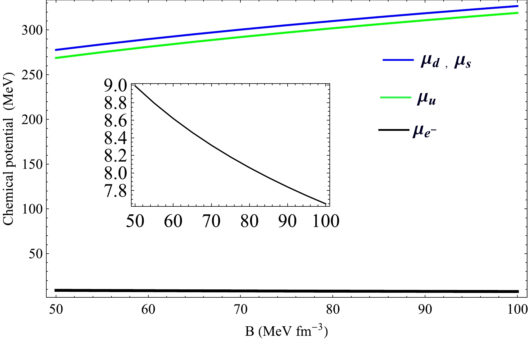
Figure 1. (color online) Plot of chemical potentials with bag constant (B) for strange quark mass
$ m_{s}=100 $ $\rm MeV$ .$ n_{b}=\frac{1}{3} \sum\limits_{{j = u,d,s}} n_{j}. $

(21) We show the variation in
$ E_{B} $ with B for different values of$ m_{s} $ in Fig. 2, and it is noted that the value of B is limited by the value of$ m_{s} $ for the different stability windows of three flavor quark matter, as tabulated in Table 1.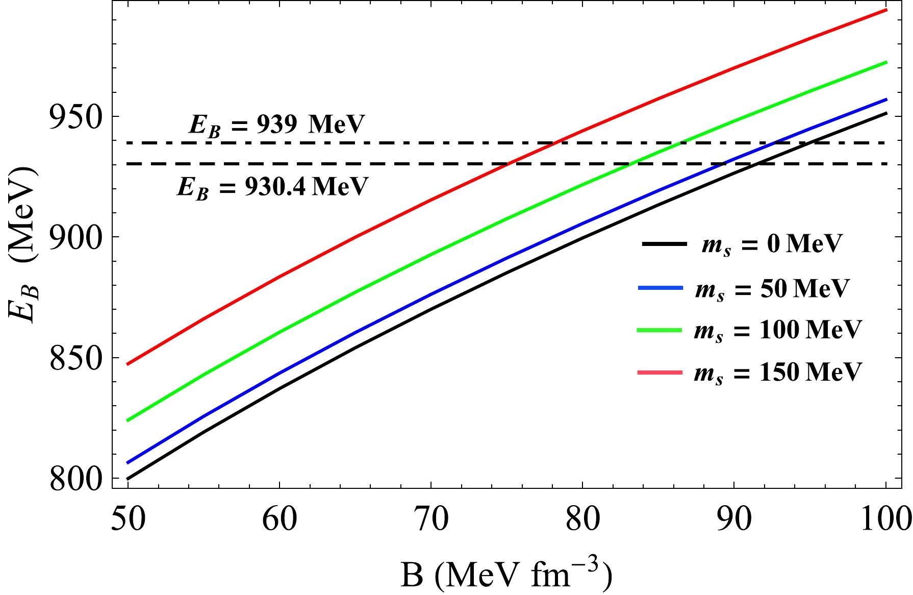
Figure 2. (color online) Plot of
$ E_{B} $ of three flavor SQM with B for different$ m_{s} $ at zero external pressure. The dot dashed line represents the mass of the nucleon, and the dashed line represents the binding energy per nucleon of$^{56}{\rm Fe}$ .$E_{B}/\rm MeV$ 

$m_{s}=0~\rm MeV$ 

$m_{s}=50~\rm MeV$ 

$m_{s}=100~\rm MeV$ 

$m_{s}=150~\rm MeV$ 

Stable $E_{B}\leq 930.4$ 

$B \leq 91.54$ 

$B \leq 89.25$ 

$B \leq 83.21$ 

$B \leq 75.12 $ 

Metastable $930.4 \leq E_{B} \leq 939$ 

$91.54 \leq B \leq 94.97$ 

$89.25 \leq B \leq 92.70$ 

$83.21 \leq B \leq 86.47$ 

$75.12 \leq B \leq 78.18$ 

Unstable $E_{B} > 939$ 

$B>94.97$ 

$B>92.70$ 

$B>86.47$ 

$B>78.18$ 

Table 1. Values of B (
$\rm MeV/fm^{3}$ ) for which${\rm SQM}$ may be stable, metastable, and unstable for different strange quark masses,$m_{s}=0,~50,~100,~150$ $\rm MeV$ . -
The interior space-time of a spherically symmetric, static cold compact star is described by the following metric element:
$ {\rm d}s^{2} = -{\rm e}^{2\nu(r)}{\rm d}t^{2}+{\rm e}^{2\lambda (r)}{\rm d}r^{2}+r^{2}({\rm d}\theta^{2}+{\rm sin}^{2} \theta {{\rm d}\phi}^{2}), $

(22) where
$ \nu(r) $ and$ \lambda(r) $ are the two unknown metric functions to be determined from boundary conditions. The energy-momentum tensor for the interior matter content of an ultra compact star in four-dimensional space-time with fluid pressure anisotropic in nature is given by the general form$ T_{\rm lm} = \rm{diag}\; (\rho, -p_{r}, -p_{t}, -p_{t}), $

(23) where ρ represents energy density, and
$ p_{r} $ and$ p_{t} $ represent the pressure along the radial and transverse directions, respectively. The EFE in four-dimensional space-time is given by$ {\bf{R}}_{\rm lm}-\frac{1}{2}g_{\rm lm}{\bf{R}} = -\frac{8\pi G}{c^2} \; {\bf{T}}_{\rm lm}, $

(24) where G denotes the Newtonian gravitational constant, and
$ R_{\rm lm} $ and R are known as the Ricci tensor and Ricci scalar, respectively. Inserting Eqs. (22) and (23) into Eq. (24), the EFE reduces to the following set of equations:$ \frac{(1-{\rm e}^{-2\lambda})}{r^{2}}+\frac{2\lambda^{\prime}{\rm e}^{-2\lambda}}{r}= \frac{8\pi G}{c^2} \rho, $

(25) $ \frac{2\nu^{\prime}{\rm e}^{-2\lambda}}{r}-\frac{(1-{\rm e}^{-2\lambda})}{r^2}= \frac{8\pi G}{c^2}p_{r}, $

(26) $ {\rm e}^{-2\lambda}\left[\nu ^{\prime \prime }+{\nu ^{\prime }}^{2}-\nu ^{\prime }\lambda ^{\prime }-\frac{(\lambda ^{\prime}-\nu ^{\prime })}{r}\right] = \frac{8\pi G}{c^2}p_{t}, $

(27) Using Eqs. (26) and (27), we get the following equation:
$ {\rm e}^{-2\lambda}\left[\nu ^{\prime \prime }+{\nu ^{\prime }}^{2}-\nu ^{\prime }\lambda ^{\prime }-\frac{\nu ^{\prime }}{r}- \frac{\lambda ^{\prime}}{r}-\frac{(1-{\rm e}^{2\lambda})}{r^2}\right] = \frac{8\pi G}{c^2}\Delta. $

(28) Here,
$ \Delta=p_{t}-p_{r} $ is the measure of pressure anisotropy. Clearly, the anisotropy depends on the metric potentials$ \nu(r) $ and$ \lambda(r) $ . The superscript dash$ (') $ denotes the derivative w.r.t the radial co-ordinate r. To solve Eqs.$(25)- (28)$ , we consider the modified form of the Finch-Skea metric [64] for the interior space-time by introducing one extra parameter α in the metric potential${\rm e}^{2\nu(r)}$ , as given below.$ {\rm e}^{2\lambda(r)}=(1+Cr^2), $

(29) $ \begin{aligned}[b] {\rm e}^{2\nu(r)} =& \left[ \left\{(F+S \sqrt{(1-\alpha)(1+Cr^2)})\right\} {\rm sin}\sqrt{(1-\alpha)(1+Cr^2)} \right. \\ &\left. +\left\{S-F \sqrt{(1-\alpha)(1+Cr^2)}\right\} {\rm cos}\sqrt{(1-\alpha)(1+Cr^2)}\right]^{2}, \end{aligned} $

(30) where α accounts for the anisotropy parameter, and when
$ \alpha=0 $ , the original Finch-Skea [59] metric is obtained. Here, C, F, and S are three arbitrary real constants that define the three-space of the interior matter of stars, which are calculated using the boundary conditions. The expressions for energy density (ρ), radial pressure$ (p_{r}) $ , transverse pressure$ (p_{t}) $ , and pressure anisotropy$ (\Delta) $ are relevant to this model via$ \rho=\frac{C[3+Cr^2]}{8\pi G Y^2}, $

(31) $ p_{r}=\frac{C [{\rm sin}K (F(1-2\alpha)-SK)+{\rm cos}K(S(1-2\alpha)+FK)]}{8\pi G X Y}, $

(32) $ \Delta=\frac{\alpha C^2r^2}{8\pi GY^2} $

(33) and
$ p_t = p_r + \Delta, $

(34) where
$ Y=1+Cr^2 $ ,$X=(S-FK)\; {\rm cos}(K) +(F+SK)\; {\rm sin}(K)$ , and K =$ \sqrt{(1-\alpha)(1+Cr^2)} $ . Equations (29) – (34) are used to determine the physical properties of a compact star. In the subsequent sections, we consider$ c=1 $ and$ 8 \pi G=1 $ . -
To obtain various physical parameters in this model, we impose the boundary conditions given below.
(a) The interior solution obtained from the model should be continuous throughout the star and matched to Schwarzschild's exterior solution at the stellar surface (
$ r=b $ ), which is given by$ \begin{aligned}[b] {\rm d}s^{2} =& -\left(1-\frac{2M}{r}\right){\rm d}t^{2}+\left(1-\frac{2M}{r}\right)^{-1}{\rm d}r^{2}\\&+r^{2}({\rm d}\theta^{2}+ {\rm sin}^2\theta{{\rm d}\phi}^{2}), \end{aligned} $

(35) where M is the gravitational mass. Therefore, if we consider the radius of a star as b, we must have
$ {\rm e}^{2\nu(r=b)}={\rm e}^{-2\lambda(r=b)}=\left(1-\frac{2M}{b}\right). $

(36) (b) At the stellar surface, radial pressure
$ (p_{b}) $ should vanish. Therefore, from Eq. (32), we determine the following expression:$ {\tan}(K_{b})=\frac{FK_{b}+ (1-2 \alpha)S}{SK_{b}-F(1-2\alpha)}, $

(37) where
$ K_{b}=\sqrt{(1-\alpha)(1+Cb^2)} $ .(c) Here, we choose the value of B in the range
$ 57.55 < B < B_{\rm{stable}}{\rm{MeV/fm^3}} $ , where$B_{\rm stable}$ is calculated with respect to$^{56}{\rm Fe}$ , below which SQM is stable at zero external pressure [12]. Using Eqs. (16) and (17) in Eq. (20), we may evaluate the value of surface energy density as$ \rho_b=4B + f_{1} $ , where$ f_{1}=\dfrac{3}{2}\dfrac{m^2_{s}\mu^2}{\pi ^2} \left[\sqrt{1-\dfrac{m^2_{s}}{\mu^2}}- \dfrac{m_{s}}{\mu} \ln{(1+\sqrt{1-\dfrac{m^2_{s}}{\mu^2}}})\right] $ . This value of$ \rho_{b} $ is thenused to evaluate an upper limit on the radius thatmay exist for which stable strange matter may be realized for$ m_{s}\ne0 $ . To obtain this bound, we first evaluate the condition necessary to ensure that the constant C in Eq. (29) is real. This makes the metric potential${\rm e}^{2\lambda(r)}$ real. The value of C can be calculated from Eq. (31) when the surface energy density ($ \rho_b $ ) and radius (b) of a compact object are given. From Eq. (31), we note the value of the constant C,$ C=\frac{(2 b^2 \delta -3) \pm \sqrt{(9 - 8 b^2 \delta)}}{2 b^2(1-b^2 \delta)}. $

(38) The quantity
$ (9 -8b^2\delta)\ge0 $ so that the constant C in Eq. (38) is real. Here,$ \delta=\dfrac{4B+f_{1}}{(197.3)^3 \times 3 \times 10^4 } $ is a constant that depends on B,$ m_{s} $ , and μ. Hence, when we consider the finite mass of a strange quark, the radius (b) of the star depends on B,$ m_{s} $ , and μ. Therefore, the necessary and sufficient condition to ensure that the metric function${\rm e}^{2\lambda}$ is real can be written as$ b_{\rm allowed}\leq \frac{3}{2}\sqrt{\frac{1}{2\delta}}. $

(39) (d) The causality condition must hold at all interior points and the surface for a physically viable stellar model. This condition defines that
$ 0 \leq v_{r}^2 \leq 1 $ and$ 0\leq v_{t}^2 \leq 1 $ . This is alternatively equivalent to the relations$0\leq(\dfrac{{\rm d}p_{r}}{{\rm d}\rho})\leq1$ and$0\leq (\dfrac{{\rm d}p_{t}}{{\rm d}\rho})\leq1$ , respectively. -
To obtain the maximum mass of a strange quark star in this model, we first calculate the maximum radius of the star. Here, we discuss the technique used to obtain the maximum radius and corresponding maximum mass of an SS. We calculate the radius using the surface energy density
$ \rho_{b}=4B + f_{1} $ for different values of$ m_{s} $ $ (= 0 $ , 50, 100, 150 MeV$ ) $ and two values of B. The minimum and maximum values of B are taken as$B_{\rm low}=57.55\; {\rm MeV/fm^{3}}$ and$B_{\rm max}=B_{\rm stable}$ , respectively. The values of$B_{\rm stable}$ for different values of$ m_{s} $ are shown in Table 1.For a set of B and
$ m_{s} $ values, we note two values of radius$ (b) $ from Eq. (38), out of which one gives a real value of C and satisfies all physical criteria, such as$ (i) $ $(\frac{{\rm d}p}{{\rm d}\rho}) \leq 1$ , and$ (ii) $ pressure ($ p_{r} $ ) should monotonically decrease and be positive throughout the star. Within the range of B, we determine the maximum mass of the SS for different values of$ m_{s} $ $ (=0 $ , 50, 100, 150$\rm MeV)$ . The value of the maximum radius ($b_{\rm max }$ ) and corresponding maximum mass ($M_{\rm max}$ ) are calculated, as shown in Tables 2 and 3. Note that the maximum mass of the SS increases with anisotropy for fixed B and$ m_{s} $ but decreases with increasing B for fixed α and$ m_{s} $ . Moreover, the maximum mass decreases with increasing$ m_{s} $ when α and B are fixed. We also study the dependence of the mass of a strange quark star (M) with B for different fixed radii (b) and$ m_{s} $ . We find that the mass of a strange quark star increases with B, as shown in Fig. 3.${m_{s}/\rm MeV}$ 

anisotropy (α) $B_{\rm min}(=57.55 \;{\rm MeV /fm^{3}})$ 

$b_{\rm max}/\rm km$ 

$M_{\rm max}(M_{\odot})$ 

$u_{\rm max}$ 

$Z_{s,\rm max}$ 

0 0 12.097 2.94 0.3599 0.8796 0.3 12.109 3.08 0.3750 1.0014 50 0 12.006 2.92 0.3589 0.8813 0.3 12.017 3.05 0.3743 0.9949 100 0 11.797 2.87 0.3590 0.8821 0.3 11.808 3.00 0.3747 0.9980 150 0 11.579 2.82 0.3586 0.8846 0.3 11.590 2.95 0.3750 1.0034 Table 2. Maximum mass (
$M_{\rm max}$ ), radius ($b_{\rm max}$ ), compactness ($u_{\rm max}$ ), and surface red-shift$(Z_{s,{\rm max}})$ of a strange star for different strange quark masses,$ m_{s}=0,~ 50,~100,~150 $ $\rm MeV$ , and anisotropy (α).$B=57.55\; {\rm MeV/fm^3}$ .${m_{s}/\rm MeV}$ 

anisotropy (α) $B_{\rm stable}(\rm MeV/fm^3)$ 

$b_{\rm max}/\rm km$ 

$M_{\rm max}(M_{\odot})$ 

$u_{\rm max}$ 

$Z_{s,{\rm max}}$ 

0 0 9.522 2.33 0.3589 0.8961 0.3 9.670 2.46 0.3750 1.0018 50 0 9.660 2.39 0.3590 0.9240 0.3 9.664 2.46 0.3750 1.003 100 0 9.844 2.40 0.3590 0.8822 0.3 9.854 2.50 0.3745 0.9964 150 0 10.168 2.47 0.3589 0.8785 0.3 10.177 2.60 0.3735 1.0148 Table 3. Maximum mass (
$M_{\rm max}$ ), radius ($b_{\rm max}$ ), compactness ($u_{\rm max}$ ), and surface red-shift$(Z_{s,\rm max})$ of a strange star for different strange quark masses,$ m_{s}=0, 50,100,150 $ $\rm MeV$ , and anisotropy (α).$B=B_{\rm stable}$ , as given in Table 1.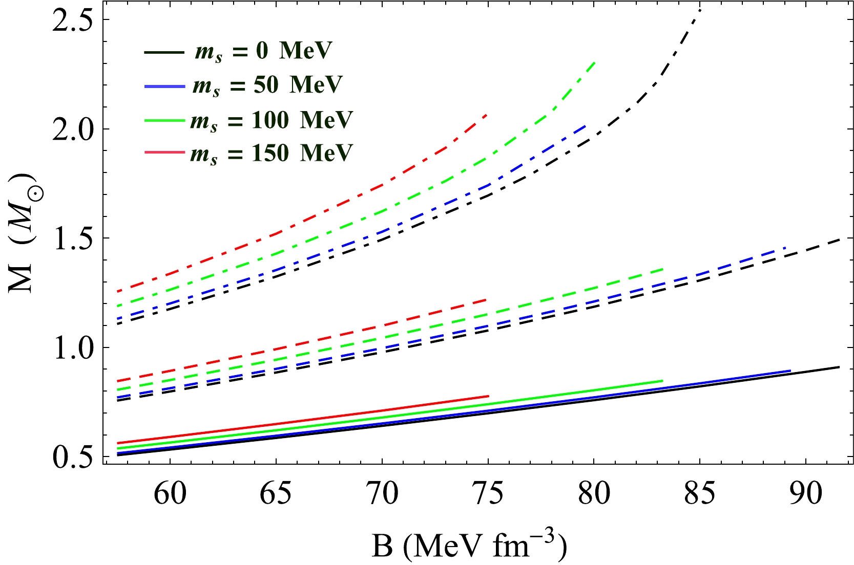
Figure 3. (color online) Variations in mass
$ M(M_{\odot}) $ with B ($57.55 \leq B \leq B_{\rm stable}\; \rm MeV/fm^{3}$ ). The solid, dashed, and dot dashed lines represent data at radius$ b=8,9,10 $ km, respectively. -
The gravitational mass of compact objects is obtained as
$ M(b) = 4\pi \int^{b}_{0}\rho(r^{\prime})r^{\prime{2}} {\rm d} r^{\prime} = \frac{C b^{3}}{2(1+C b^{2})}, $

(40) where
$ \rho(r^{\prime}) $ is the energy density at any radial distance$ r^{\prime} $ , and b is the radius of the star. Using Eq. (31), we numerically obtain the mass-radius relationship upto maximum radius ($b_{\rm max}$ ) for different strange quark masses ($ m_{s} $ ) and two values of the bag constant,$B= 57.55 \rm MeV/fm^{3}$ and$B=B_{\rm stable}$ . The radial variation in mass is shown in Fig. 4. The compactness u of the star is given by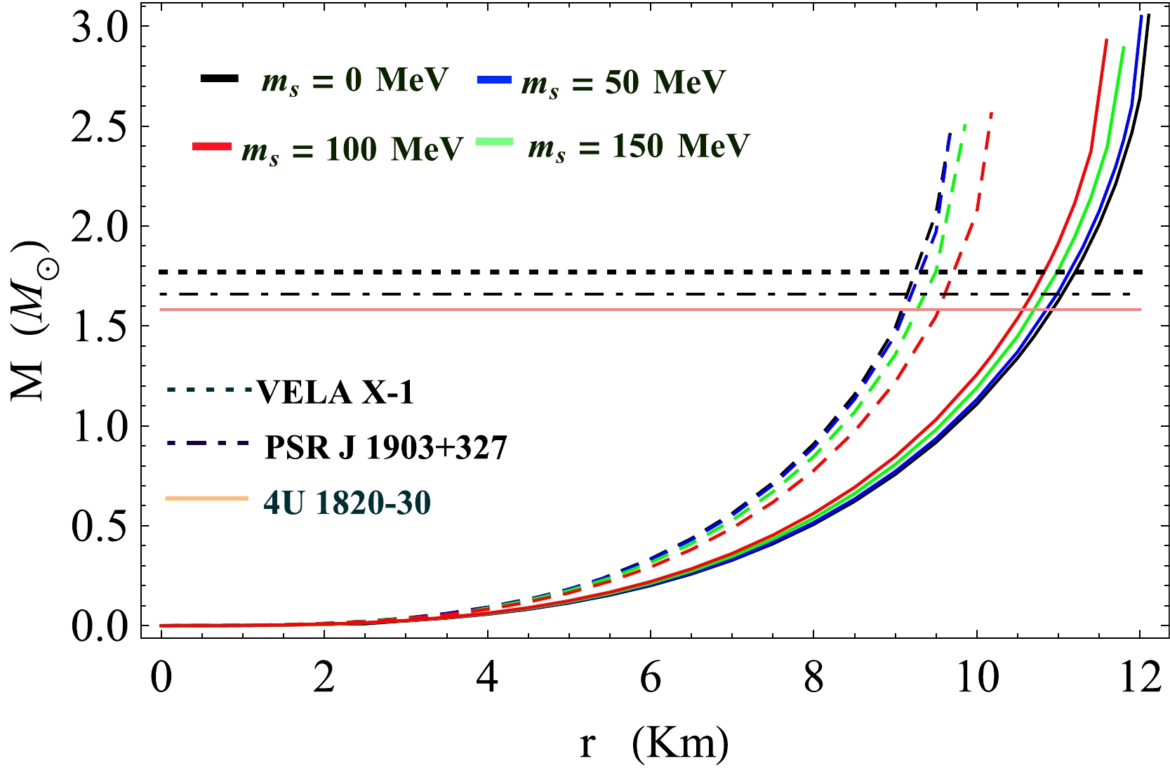
Figure 4. (color online) Variations in
$ M(M_{\odot}) $ with radial distance$ (r) $ . The solid and dashed lines represent$ B=57.55 $ $\rm MeV/fm^{-3}$ and$B= B_{\rm stable}$ , respectively, when$ \alpha=0.0 $ .$ u=\frac{M(b)}{b}= \frac{C b^{2}}{2(1+C b^{2})}. $

(41) The surface red-shift (
$ Z_{s} $ ) corresponding to the compactness (u) can be obtained as [71]$ \begin{eqnarray} Z_{s}=\left[1-(2u)\right]^{-\frac{1}{2}}-1=\sqrt{\frac{1}{1+Cb^{2}}}-1 . \end{eqnarray} $

(42) From Eqs. (40) and (41), we find that both the mass and compactness will be maximum when
$b=b_{\rm max}$ and y$ (=cb^2) $ is maximum. The maximum mass and maximum compactness are given by$ M_{\rm max}= \frac{ b_{\rm max}}{2\left(1+\dfrac{1}{y_{\rm max}}\right)}, $

(43) $ u_{\rm max}= \frac{1}{2\left(1+\dfrac{1}{y_{\rm max}}\right)}. $

(44) The maximum surface red-shift corresponding to the maximum compactness can be obtained from Eq. (42). The variation in maximum surface red-shift is shown in Fig. 5.
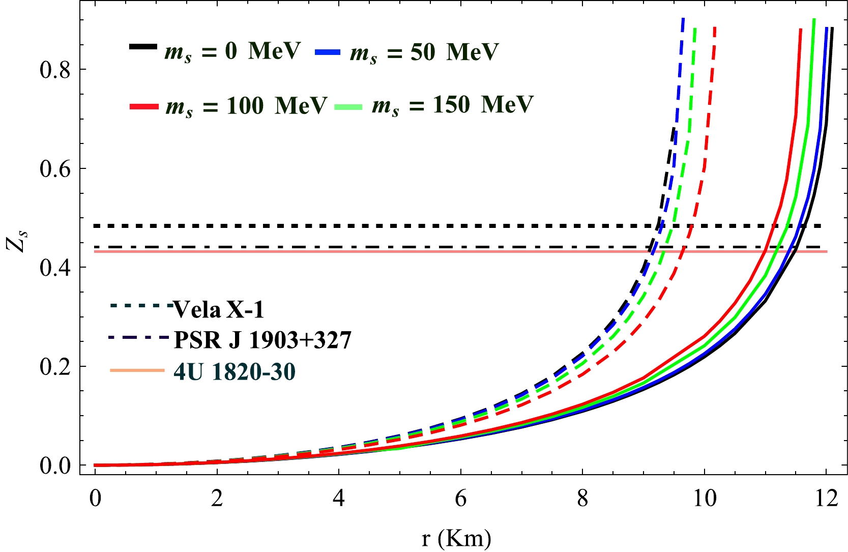
Figure 5. (color online) Variations in surface red-shift (
$ Z_{s} $ ) with radial distance$ (r) $ . The solid and dashed lines represent$ B= 57.55 $ $\rm MeV fm^{-3}$ and$B=B_{\rm stable}$ , respectively, when$ \alpha=0.0 $ . -
For any compact object with a known mass (M) and radius (b), the constant C in Eq. (29) can be determined using the boundary condition in Eq. (36). Because C is known, simultaneously solving Eqs. (36) and (37) yields the values of constants F and S for different anisotropy parameters (α). Now, we can evaluate the radial variations in physical parameters, such as ρ,
$ p_{r} $ ,$ p_{t} $ , and Δ, related to compact stars. To study the effect of B and$ m_{s} $ on the mass of strange quark stars, we adopt a different approach in which the surface energy density$ \rho_{b} $ is taken as$ \rho_{b}=4 B + f_{1} $ , where$ f_{1} $ is related to the mass and chemical potential of the strange quark, as discussed earlier. By simultaneously solving Eqs. (16) and (19) for a given B and$ m_{s} $ along with the condition that$ \sum{p_{j}}=B $ at the surface, we determine the values of the chemical potential$ \mu_{e^{-}} $ and μ. The following three stars are considered for physical analysis, which are thought to be SSs:Case I: We first consider VELA X-1, which has an observed mass
$ M=1.77 M_{\odot} $ and radius$ b=9.56 $ km [72]. The possibility of VELA X-1 lying in the SS family may be understood if the observed mass or radius can be predicted using the values of B and$ m_s $ necessary for stable SQM. In Table 4, we present the predicted radius of VELA X-1 for different values of B and$ m_{s} $ . Note that for a given B, the predicted radius increases when we include a higher value of the strange quark mass ($ m_{s} $ ) into the system. The variations in all physical parameters, namely, energy density (ρ), radial pressure ($ p_{r} $ ), transverse pressure ($ p_{t} $ ), anisotropy (Δ), ($\dfrac{{\rm d}\rho}{{\rm d}r}$ ), and ($\dfrac{{\rm d}p_{r}}{{\rm d}r}$ ), are shown in Figs. 6−11, respectively.Compact star Predicted radius from our model/km $ m_{s}= 0$ MeV

$m_{s}= 50$ MeV

$m_{s}= 115$ MeV

$m_{s}=150$ MeV

$B= 91.540 \;\rm MeV/ fm^{3}$ 

$B= 89 \;\rm MeV/fm^{3}$ 

$B= 80.906 \;\rm MeV/fm^{3}$ 

$B= 75.12 \;\rm MeVfm^{-3}$ 

VELA X-1 9.294 9.345 9.562 9.752 4U 1820-30 9.104 9.163 9.359 9.539 PSR J 1903+327 9.190 9.239 9.450 9.634 Table 4. Predicted radius (b) of compact stars 4U 1820-30, VELA X-1, and PSR J 1903+327 for different strange quark masses (
$ m_{s}=0, 50,100,150 $ $\rm MeV$ ) and the corresponding maximum value of B.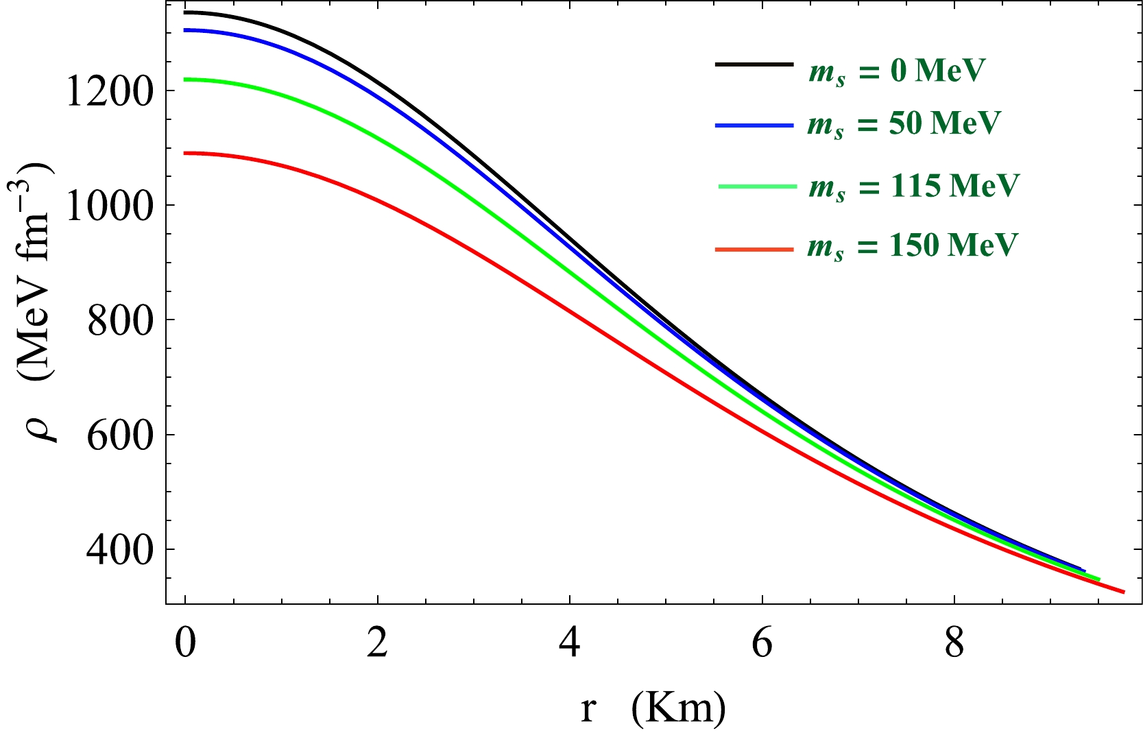
Figure 6. (color online) Plot of ρ with r /km for VELA X-1.
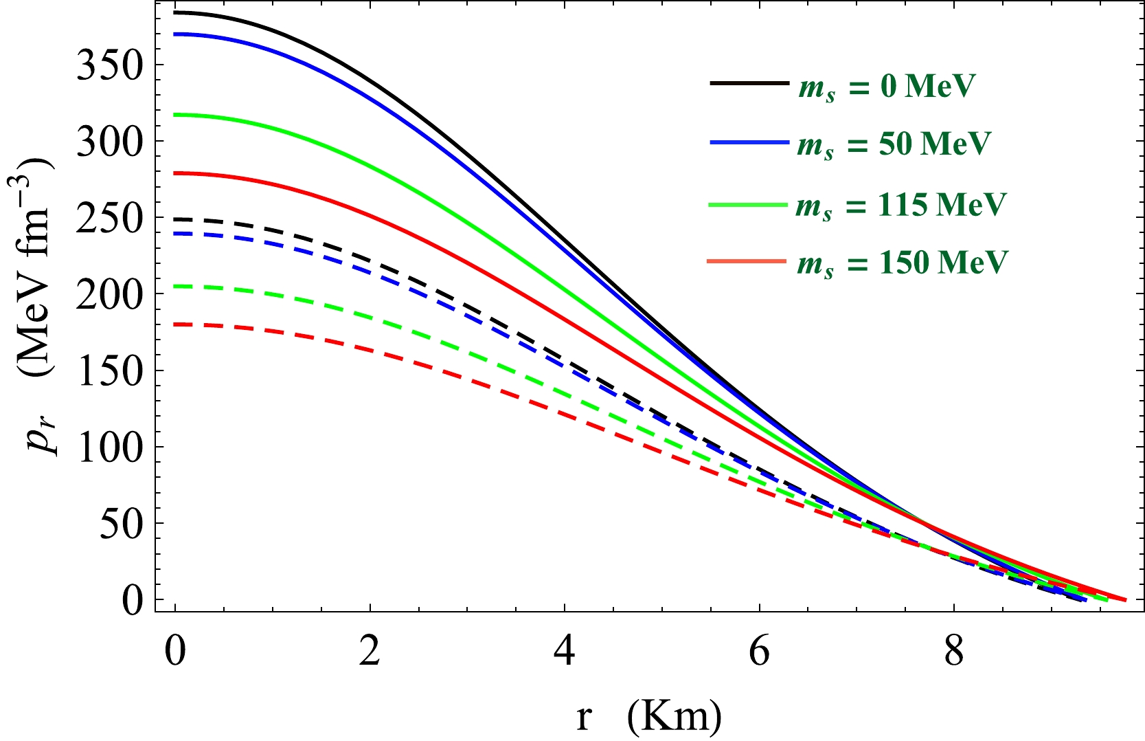
Figure 7. (color online) Plot of
$ p_{r} $ with r /km for VELA X-1. Solid line for$ \alpha=0 $ , and dashed line for$ \alpha=0.3 $ .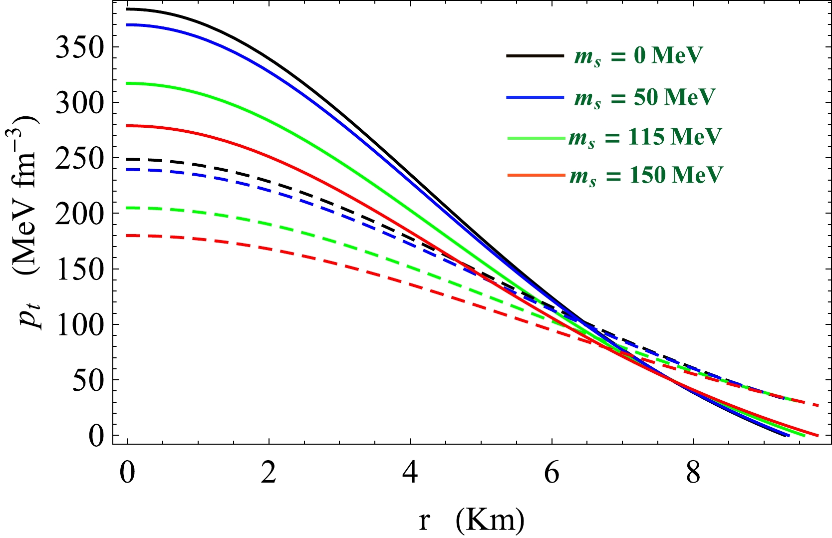
Figure 8. (color online) Plot of
$ p_{t} $ with r /km for VELA X-1. Solid line for$ \alpha=0 $ , and dashed line for$ \alpha=0.3 $ .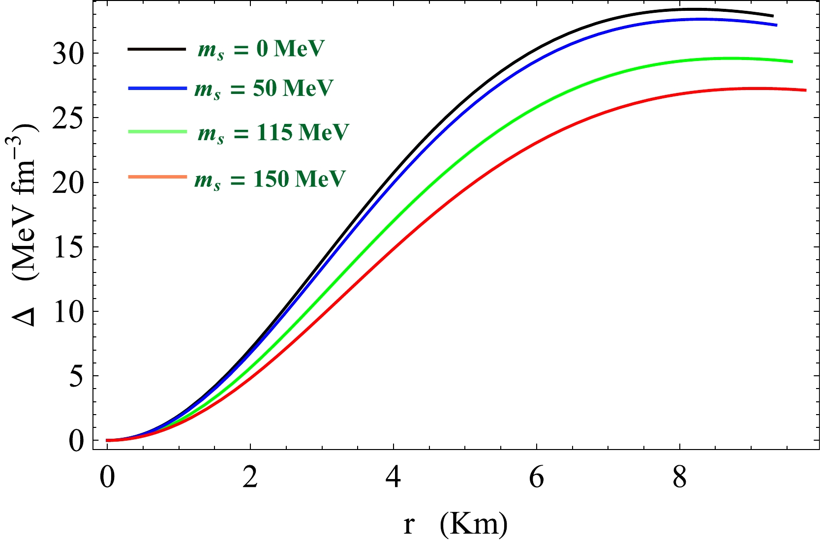
Figure 9. (color online) Plot of Δ with r /km for VELA X-1 for
$ \alpha=0.3 $ .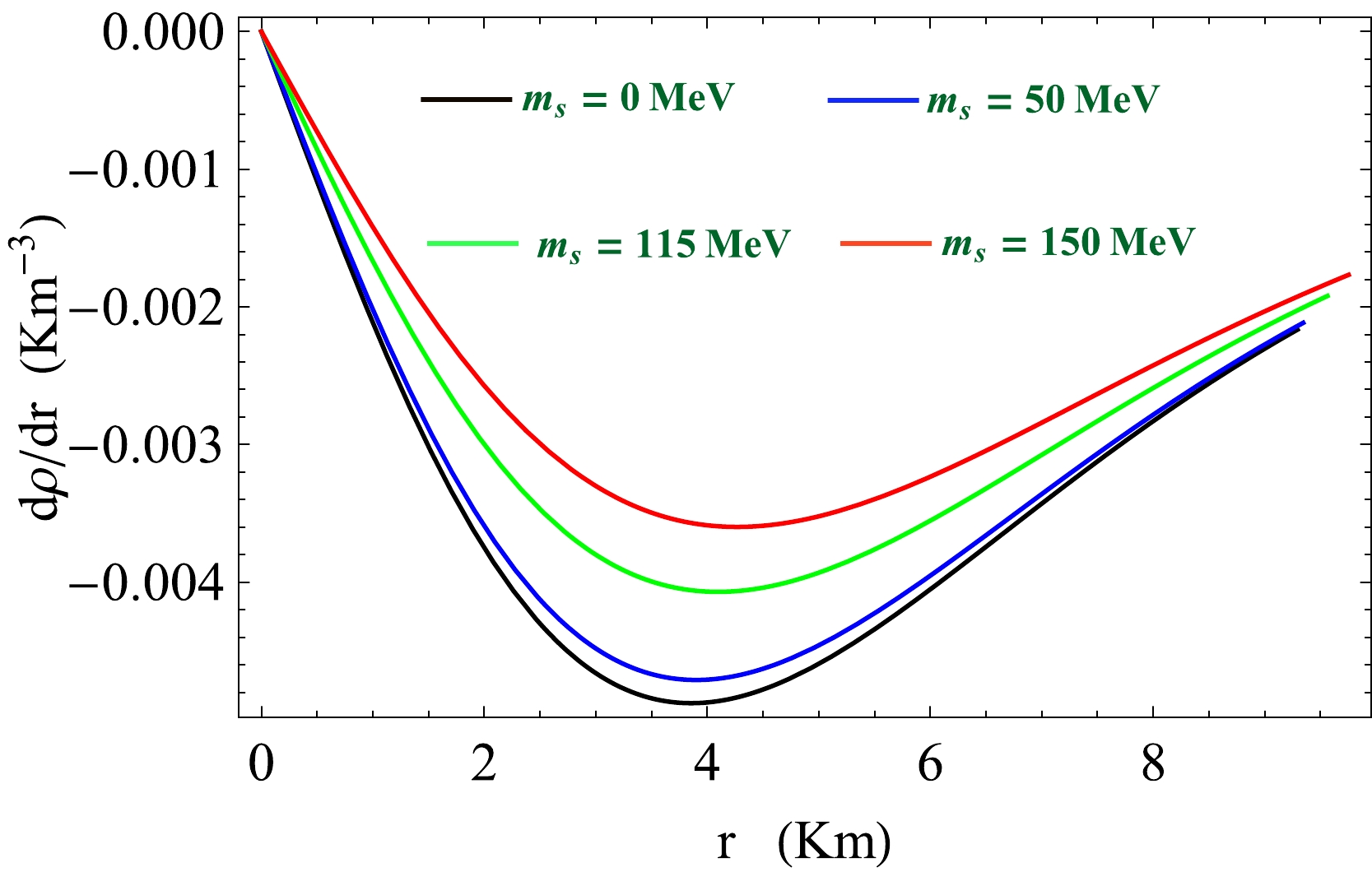
Figure 10. (color online) Plot of
$(\dfrac{{\rm d}\rho}{{\rm d}r})$ with r /km for VELA X-1.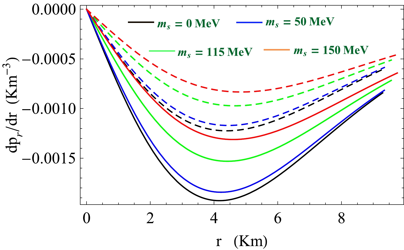
Figure 11. (color online) Plot of
$(\dfrac{{\rm d}p_{r}}{{\rm d}r})$ with r /km for VELA X-1. Solid line for$ \alpha=0 $ , and dashed line for$ \alpha=0.3 $ .Case II: Here, we consider a low mass X-ray binary, 4U 1820-30, which has an observed mass
$ M=1.58 $ $ M_{\odot} $ and radius$ b=9.1 $ km [73]. In Table 4, we present the predicted radius of 4U 1820-30 for different values of B and$ m_{s} $ . When the strange quark mass ($ m_{s} $ ) is non-zero, we can also predict the radius with a lower value of B. From Table 4, it is also noted that the predicted radius of compact objects increases when we include the higher value of the strange quark mass ($ m_{s} $ ). The plots of all physical parameters, namely, energy density (ρ), radial and transverse pressure, anisotropy (Δ), ($\frac{{\rm d}\rho}{{\rm d}r}$ ), and ($\frac{{\rm d}p_{r}}{{\rm d}r}$ ), are shown in Figs. 12−17.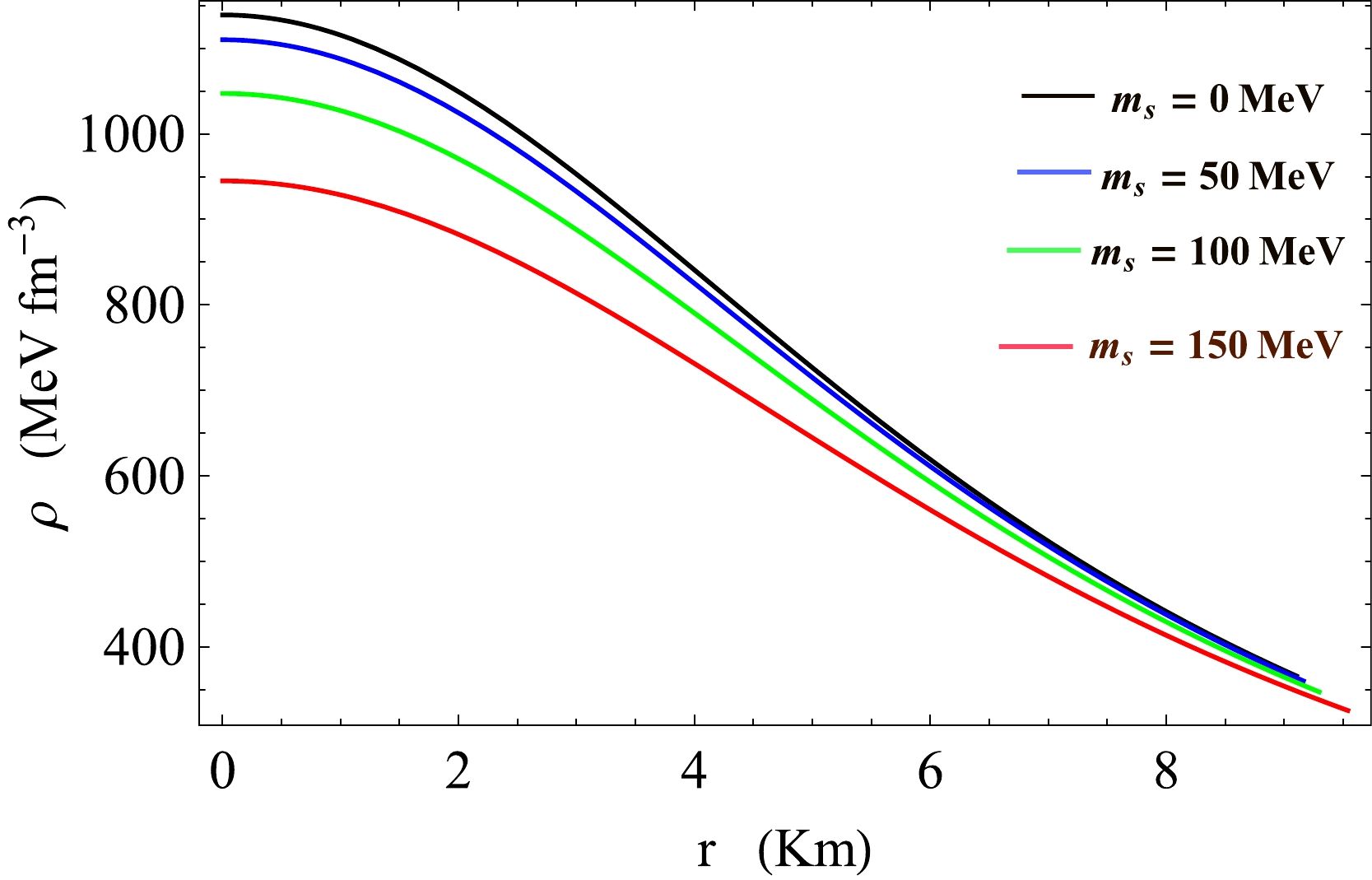
Figure 12. (color online) Plot of ρ with r /km for 4U 1820-30.
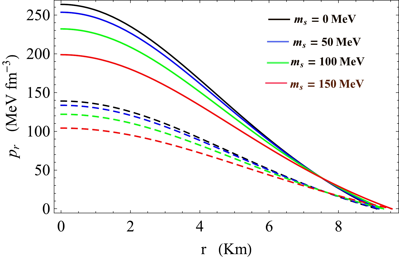
Figure 13. (color online) Plot of
$ p_{r} $ with r /km for 4U 1820-30. Solid line for$ \alpha=0 $ , and dashed line for$ \alpha=0.3 $ .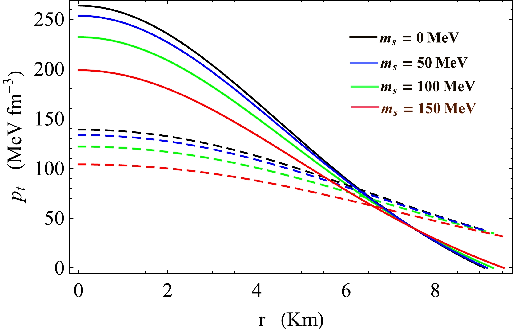
Figure 14. (color online) Plot of
$ p_{t} $ with r /km for 4U 1820-30. Solid line for$ \alpha=0 $ , and dashed line for$ \alpha=0.3 $ .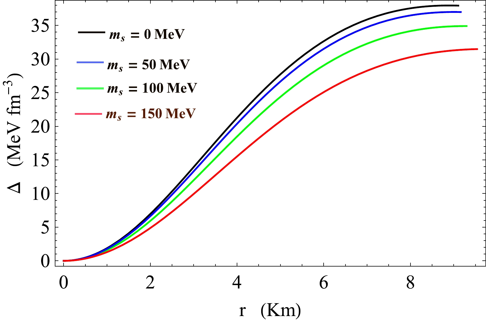
Figure 15. (color online) Plot of Δ with r /km for 4U 1820-30 for
$ \alpha=0.3 $ .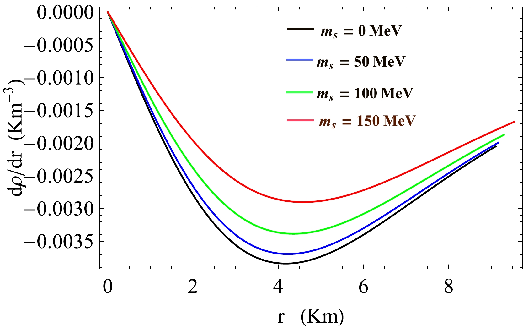
Figure 16. (color online) Plot of
$(\dfrac{{\rm d}\rho}{{\rm d}r})$ with r /km for 4U 1820-30.
Figure 17. (color online) Plot of
$(\dfrac{{\rm d}p_{r}}{{\rm d}r})$ with r /km for 4U 1820-30. Solid line for$ \alpha=0 $ , and dashed line for$ \alpha=0.4 $ .Case III: Finally, we consider the compact star PSR J 1903 +327, which has an observed mass
$ M=1.66 $ $ M_{\odot} $ and radius$ b=9.438 $ km [73]. In Table 4, we present the predicted radius of PSR J 1903+327 for different combinations of B and$ m_{s} $ . The variations in all physical parameters, namely, energy density (ρ), radial and transverse pressure, anisotropy (Δ), ($\dfrac{{\rm d}\rho}{{\rm d}r}$ ), and ($\dfrac{{\rm d}p_{r}}{{\rm d}r}$ ), are shown in Figs. 18−23.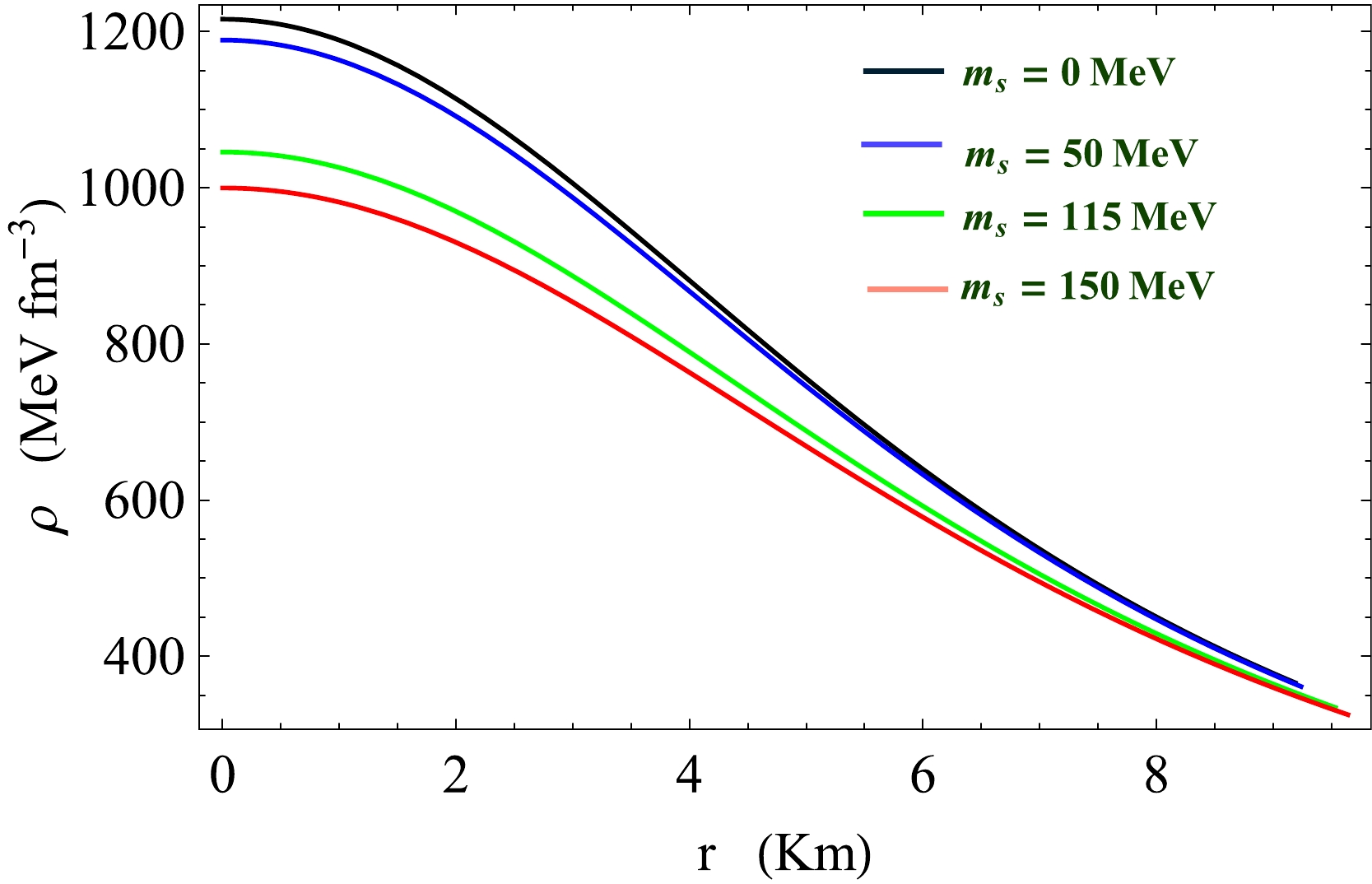
Figure 18. (color online) Plot of ρ with r /km for PSR J 1903+327

Figure 19. (color online) Plot of
$ p_{r} $ with r /km for PSR J 1903+327. Solid line for$ \alpha=0 $ , and dashed line for$ \alpha=0.3 $ .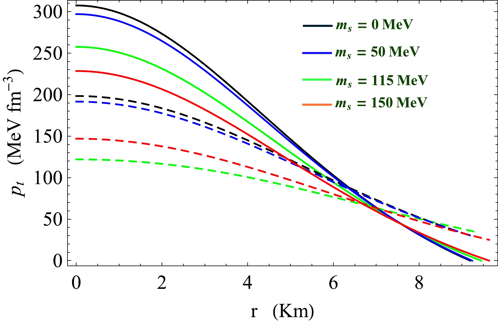
Figure 20. (color online) Plot of
$ p_{t} $ with r /km for PSR J 1903+327. Solid line for$ \alpha=0 $ , and dashed line for$ \alpha=0.3 $ .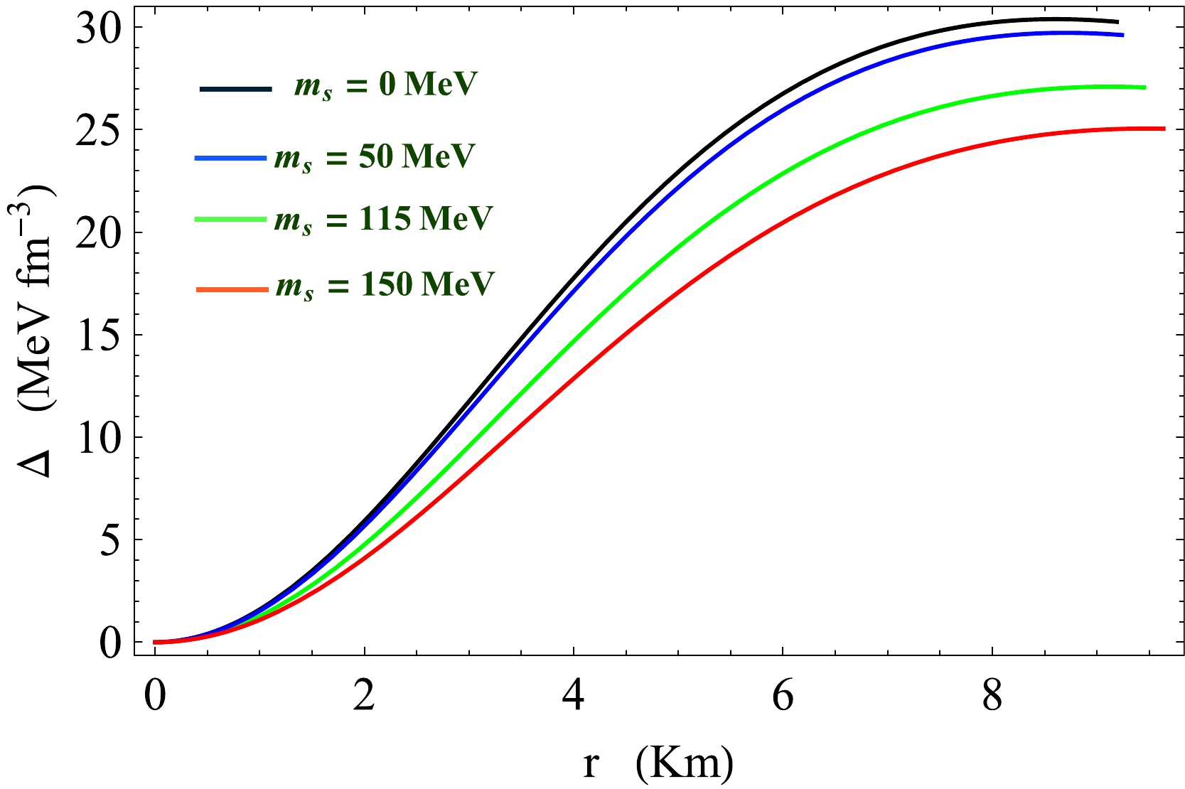
Figure 21. (color online) Plot of Δ with r /km for PSR J 1903+327.
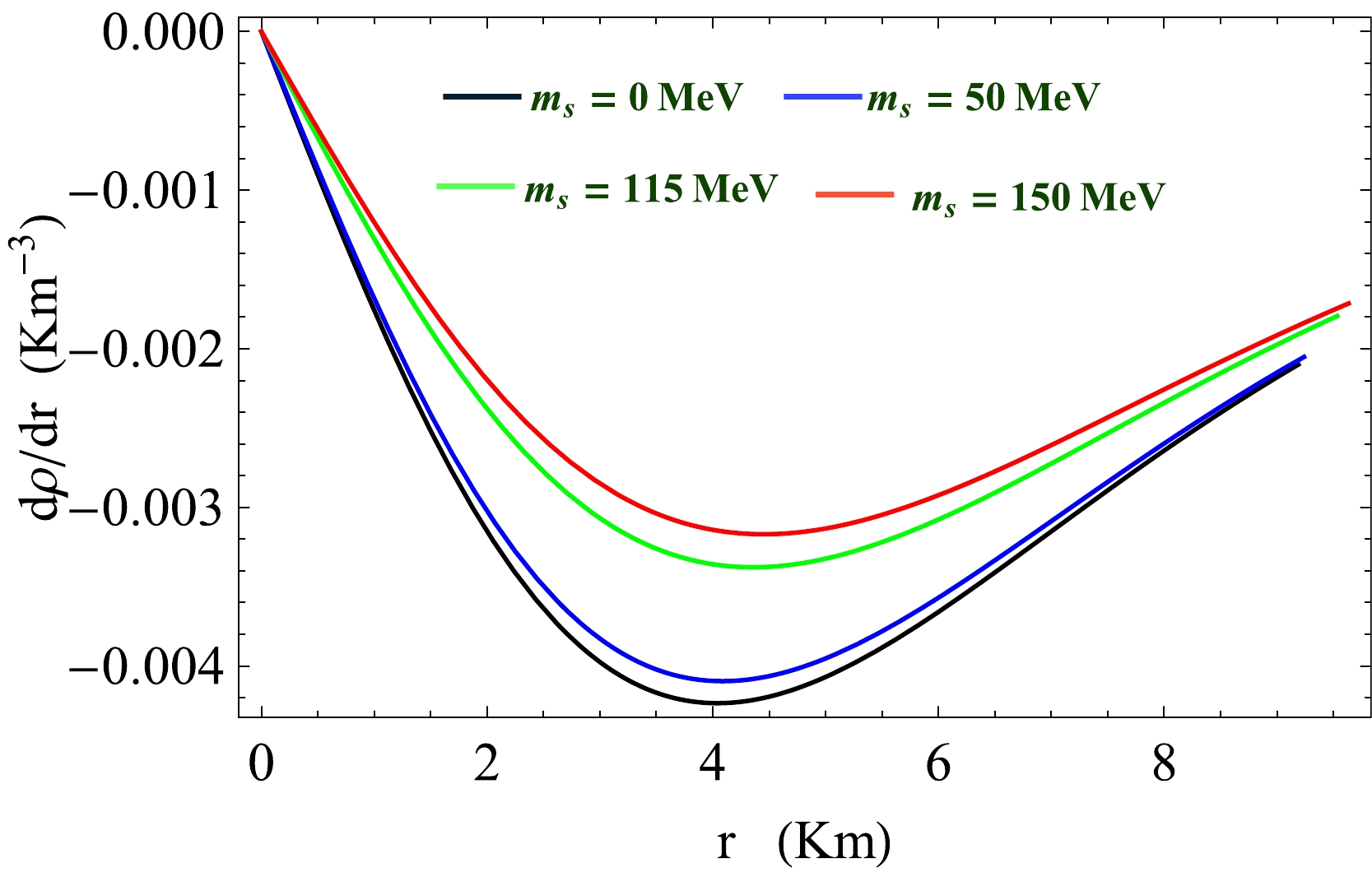
Figure 22. (color online) Plot of
$(\dfrac{{\rm d}\rho}{{\rm d}r})$ with r /km for PSR J 1903+327.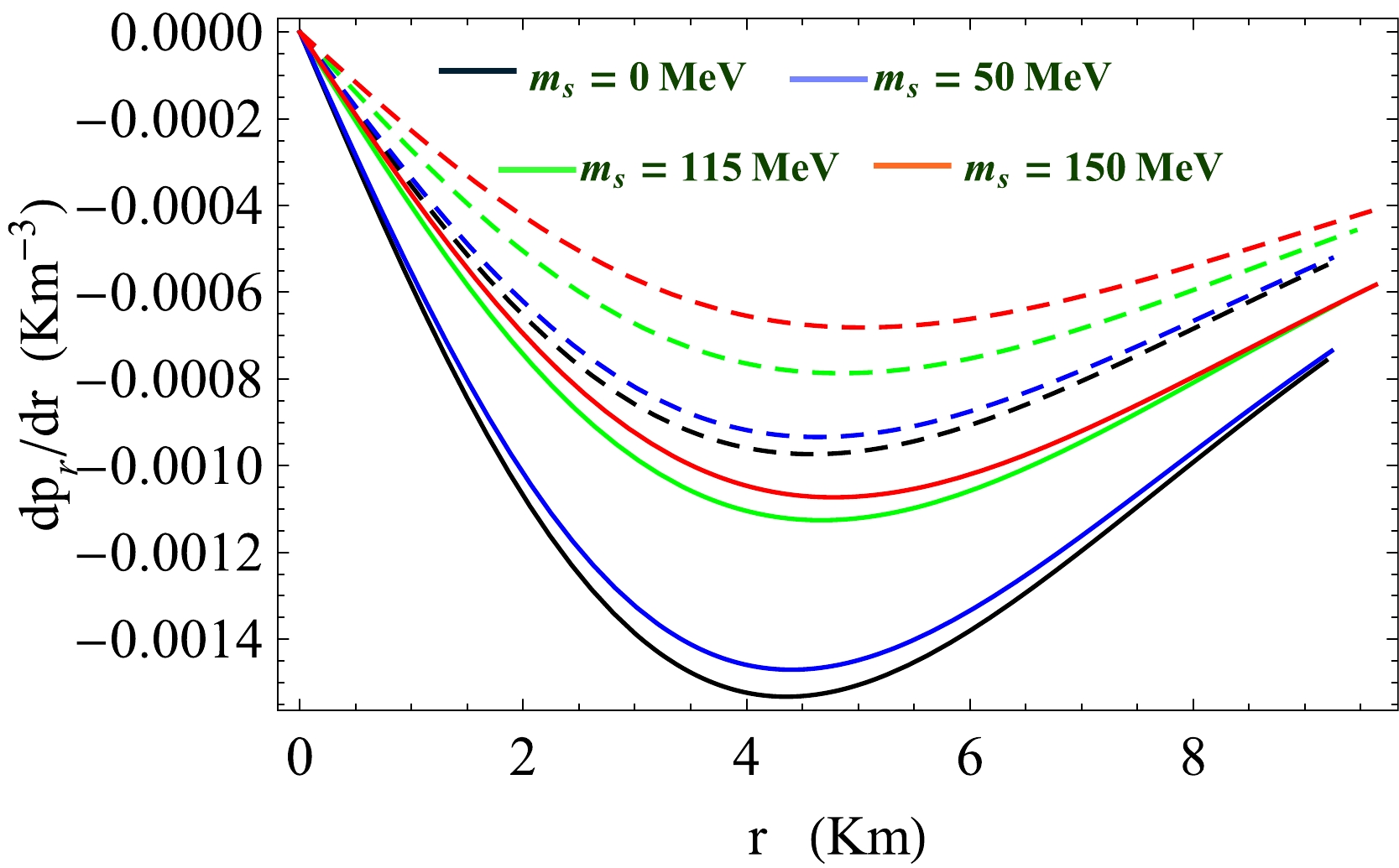
Figure 23. (color online) Plot of
$(\dfrac{{\rm d}p_{r}}{{\rm d}r})$ with r /km for PSR J 1903+327. Solid line for$ \alpha=0 $ , and dashed line for$ \alpha=0.3 $ . -
For any anisotropic fluid sphere, all the following energy conditions should be satisfied at all internal points: the mathematically strong energy condition (SEC), dominant energy condition (DEC), weak energy condition (WEC), and null energy condition (NEC), which are represented as [74, 75]
1. SEC:
$ \rho +p_{r} \geq 0, \rho +p_{t} \geq 0, \rho +p_{r}+ 2p_{t} \geq 0 $ .2. DEC:
$ \rho \geq 0, \rho -p_{r} \geq 0, \rho -p_{t} \geq 0 $ .3. WEC:
$ \rho \geq 0, \rho +p_{r} \geq 0, \rho +p_{t} \geq 0 $ .4. NEC:
$ \rho +p_{r} \geq 0, \rho +p_{t} \geq 0 $ .The energy conditions are plotted in Fig. 6 and Figs. 24−28 for VELA X-1, Fig. 12 and Figs. 24−28 for 4U 1820-30, and Fig. 18 and Figs. 24−28 for PSR J 1903+327. It is found that all the energy conditions that hold well for compact stars are considered in this study.
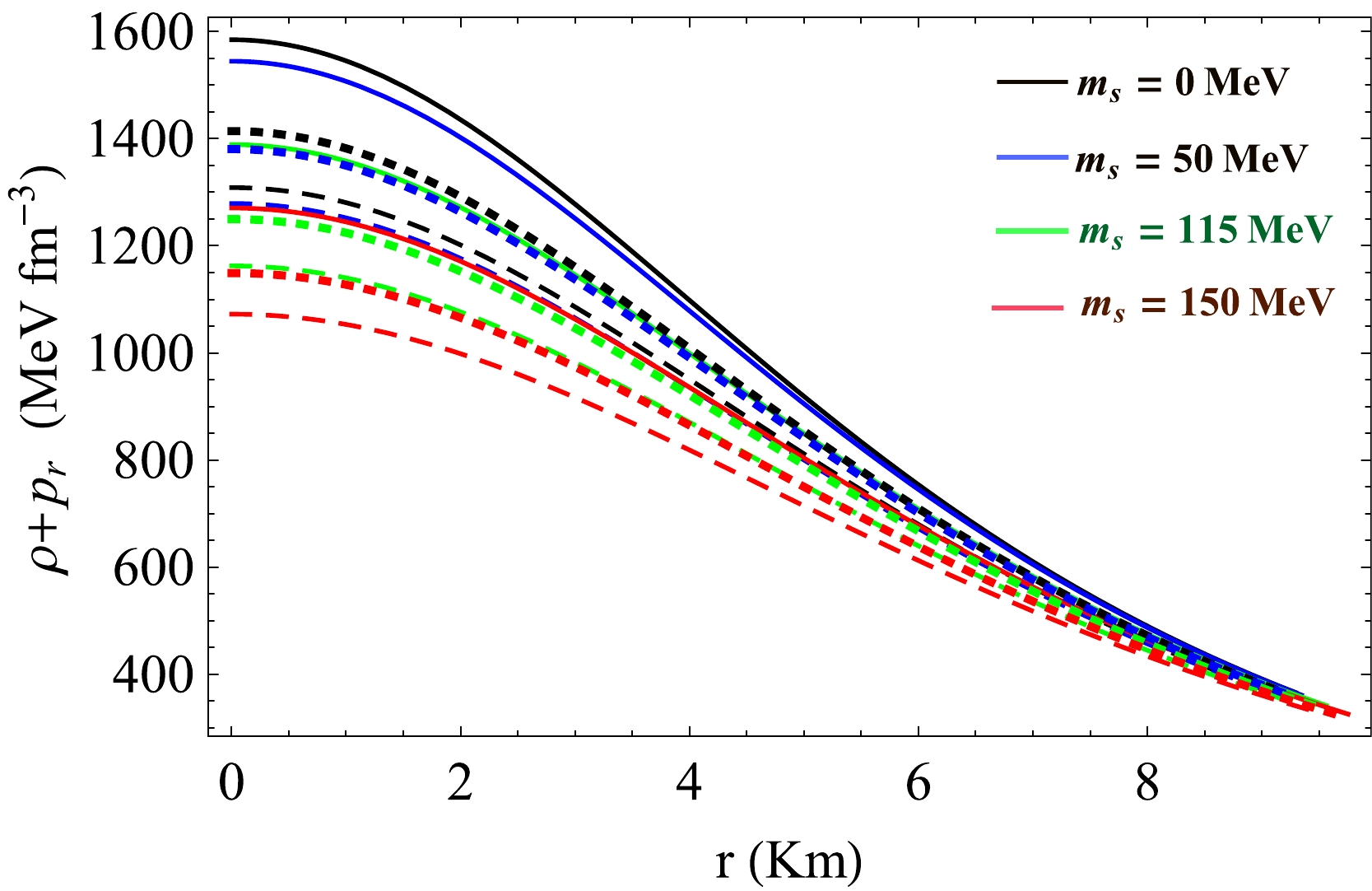
Figure 24. (color online) Plot of
$ (\rho + p_{r}) $ with r /km for$ \alpha=0.3 $ . The solid, dashed, and dotted lines represent VELA X-1, 4U 1820-30, and PSR J 1903+327, respectively.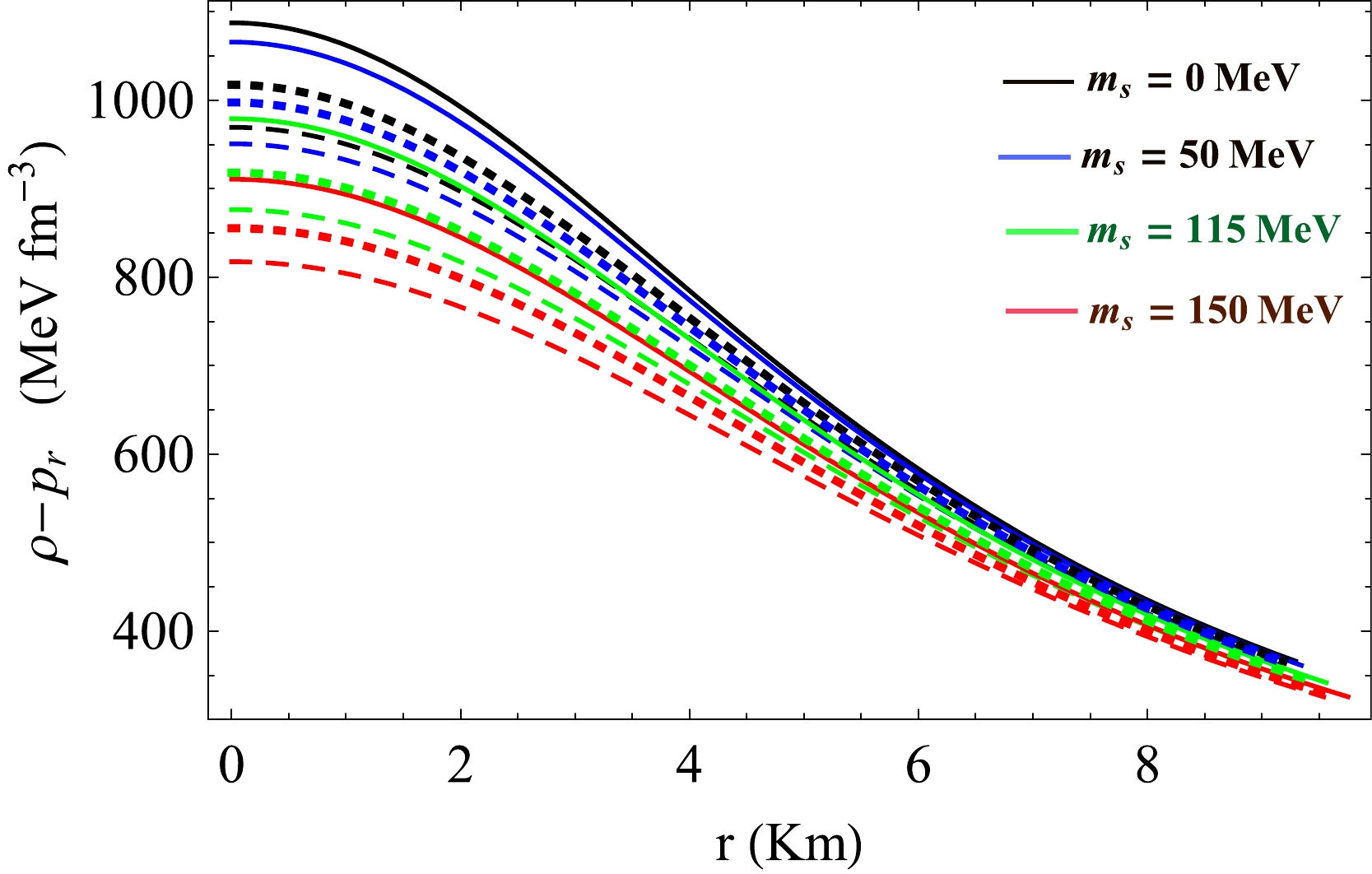
Figure 25. (color online) Plot of
$ (\rho - p_{r}) $ with r /km for$ \alpha=0.3 $ . The solid, dashed, and dotted lines represent VELA X-1, 4U 1820-30, and PSR J 1903+327, respectively.
Figure 26. (color online) Plot of
$ (\rho + p_{t}) $ with r /km for$ \alpha=0.3 $ . The solid, dashed, and dotted lines represent VELA X-1, 4U 1820-30, and PSR J 1903+327, respectively.
Figure 27. (color online) Plot of
$ (\rho - p_{t}) $ with r /km for$ \alpha=0.3 $ . The solid, dashed, and dotted lines represent VELA X-1, 4U 1820-30, and PSR J 1903+327, respectively.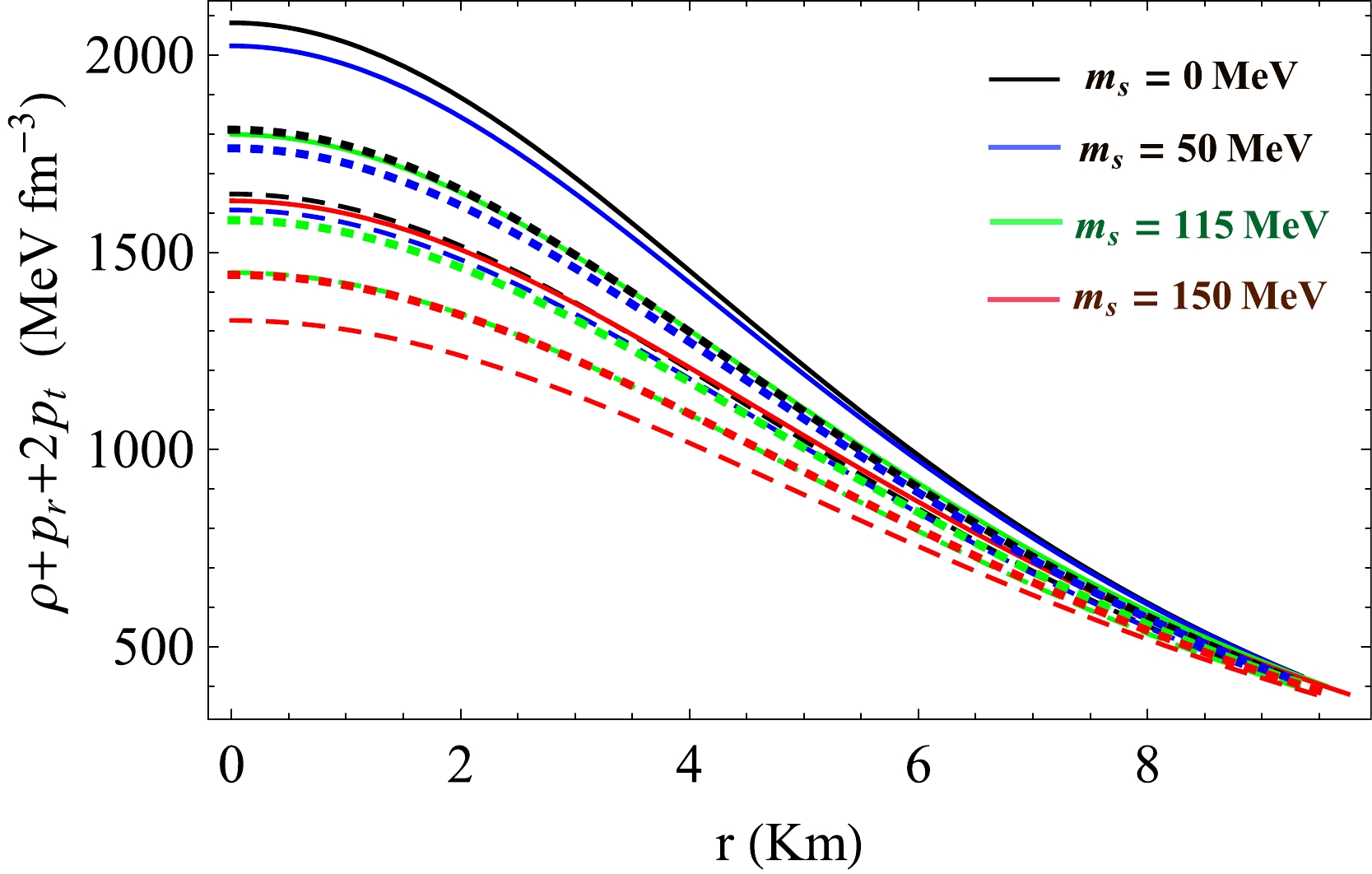
Figure 28. (color online) Plot of
$ (\rho + p_{r}+ 2 p_{t}) $ with r /km for$ \alpha=0.3 $ . The solid, dashed, and dotted lines represent VELA X-1, 4U 1820-30, and PSR J 1903+327, respectively. -
We study the nature of the Lagrangian perturbation of radial pressure with respect to the frequencies (
$ \omega^2 $ ) of normal modes at the surface to understand the stability of stellar configuration against small radial oscillations. In this context, we follow the procedure adopted by Pretel [76]. The equation governing the infinitesimal radial modes of oscillations can be represented by the following two coupled equations:$ \frac{{\rm d}\chi}{{\rm d}r}=-\frac{1}{r}\left(3\chi+\frac{\Delta p_r}{\Gamma p_r}\right)+\frac{{\rm d}\nu}{{\rm d}r}\chi, $

(45) and
$ \begin{aligned}[b] \frac{{\rm d}(\Delta p_r)}{{\rm d}r}=&\chi \left[\frac{\omega^2}{c^2}{\rm e}^{2(\lambda-\nu)}(\rho+p_r)r-4\frac{{\rm d}p_r}{{\rm d}r} \right. \\& \left.- \frac{8\pi G}{c^4}(\rho+p_r){\rm e}^{2\lambda}r p_r +r(\rho+p_r)\left(\frac{{\rm d}\nu}{{\rm d}r}\right)^2\right] \\& -\Delta p_r\left[\frac{{\rm d}\nu}{{\rm d}r}+\frac{4\pi G}{c^4}(\rho+p_r)r{\rm e}^{2\lambda}\right], \end{aligned} $

(46) where χ is known as the eigenfunction and is a function of the radial co ordinate of the Lagrangian displacement represented by the relation
$ \chi=\dfrac{\delta(r)}{r} $ . To normalize the eigenfunction$ \chi=\dfrac{\delta(r)}{r} $ at the center of the star, we consider one simple assumption that$ \chi(0)=1 $ . Apart from the previous requirement ($ \chi(0)=1 $ ), it is also evident from Eq. (45) that at$ r=0 $ , Eq. (45) possesses singularity. Therefore, the term containing the factor ($ \frac{1}{r} $ ) in Eq. (45) should vanish when$ r\rightarrow 0 $ .This argument gives another condition,
$ \Delta p_{r} = -3\lambda \chi p_r \;\; {\rm as}\;\; r\rightarrow 0. $

(47) Again, at the surface of a star, (
$ r=b $ ) as$ p_{r}(b)=0 $ , the Lagrangian perturbation of the radial pressure along the radial direction also vanishes as$ r \rightarrow b $ , that is,$ \Delta p_r=0 \;\; {\rm as} \;\; r\rightarrow b. $

(48) Here, we take the surface density
$ \rho_{b}=4 B+f_{1} $ for different values of B and$ m_{s} $ for which SQM is stable. To evaluate$ |\Delta p_r(b)| $ , we solve the coupled Eqs. (45) and (46) for different combinations of ω using the boundary condition given by Eq. (47) along with the normalization condition$ \chi(0)=1 $ . We show the variation in the Lagrangian perturbation of the radial pressure along the radial direction$ (|\Delta p_r(b)|) $ with$ \omega^2 $ in Figs. 29, 30, and 31 for VELA X-1, 4U 1820-30, and PSR J 1903+327, respectively. The correct values of the normal mode frequencies are represented by the corresponding minima of these plots. From Figs. 29−31, it is noted that all normal mode frequencies are positive, that is,$ \omega_{n}^2>0 $ . Thus, from the above analysis, it is evident that the model is stable with respect to small radial perturbations.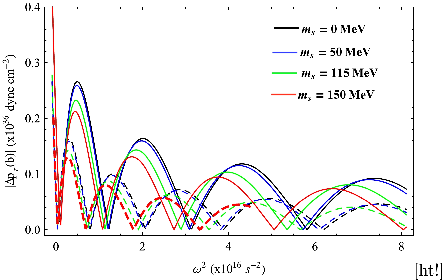
Figure 29. (color online) Plot of
$ |\Delta p_{r}(b)| $ with the frequencies$ (\omega^2) $ of normal modes at the surface of the star VELA X-1 for$B = 89.246\; \rm MeV/fm^3$ (Table 1). Solid lines for$ \alpha=0.0 $ , and dashed lines for$ \alpha=0.3 $ .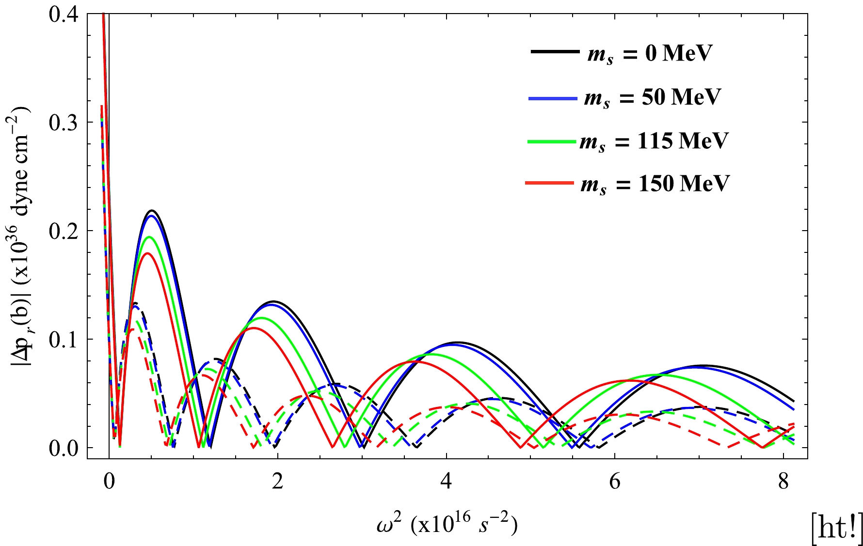
Figure 30. (color online) Plot of
$ |\Delta p_{r}(b)| $ with the frequencies$ (\omega^2) $ of normal modes at the surface of the star 4U 1820-30 for$B = 89.246\; \rm MeV/fm^3$ (Table 1). Solid lines for$ \alpha=0.0 $ , and dashed lines for$ \alpha=0.3 $ .
Figure 31. (color online) Plot of
$ |\Delta p_{r}(b)| $ with the frequencies$ (\omega^2) $ of normal modes at the surface of the star PSR J 1903+327 for$B = 89.246\; \rm MeV/fm^3$ (Table 1). Solid lines for$ \alpha=0.0 $ , and dashed lines for$ \alpha=0.3 $ . -
The EoS represents the connection between the energy density and pressure of a thermodynamic system. If we consider compact objects composed of the de-confined phase of quarks, the linear form of the EoS may be useful to study the properties discussed in Refs. [77−79]. In this paper, we analyze the impact of a finite value of
$ m_{s} $ on the EoS of SQM in the stable region. The EoS of the interior matter of the three stars VELA X-1, PSR J 1903+327, and 4U 1820-30 for finite strange quark mass$ m_{s}=50 $ MeV is shown in Fig. 32, and it is evident that forms of the EoS are linear. Therefore, ourmodel is also suitable for the study of other stars in the SS family.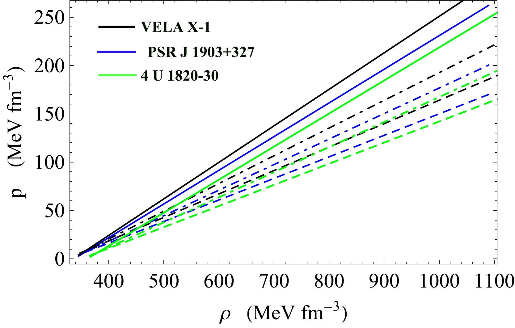
Figure 32. (color online) Plot of p vs ρ of the interior matter of VELA X-1, PSR J 1903+327, and 4U 1820-30 when
$ m_{s}=50 $ MeV. The solid, dot-dashed, and dashed lines represent$ \alpha=0.0, $ $ 0.2 $ , and$ 0.3 $ , respectively. -
In this paper, a class of anisotropic strange quark stars in the context of modified Finch-Skea geometry [65] is presented, and the predicted maximum mass, radius, and stability of strange quark stars composed of de-confined three-flavor quarks are discussed qualitatively. We consider the EoS of interior matter as the MIT EoS in the presence of a finite value of strange quark mass (
$ m_{s}\neq0 $ ). It is evident from Fig. 1 that the chemical potential of the electron is significantly smaller than that of u, d, and s quarks. To define the stability window of bulk quark matter, the energy per baryon is evaluated and shown in Fig. 2 for different values of B and$ m_{s} $ . It may be concluded that$ m_{s} $ and B have an effect on$ E_{B} $ and the overall stability of the system. We investigate the effect of a finite value of strange quark mass ($ m_{s} $ ) on the value of the maximum mass of strange quark stars, considering the range of B from$ B=57.55 $ to$B=B_{\rm stable}\; \rm (MeV/fm^{3})$ , and note some interesting results, where$B_{\rm stable}$ is the maximum allowed value of B for which$ E_{B} \leq 930.4 $ MeV relative to$^{56} \rm Fe$ shown in Table 1 is evaluated from Fig. 2. From Eq. (39), it is noted that for stable strange quark stars, the allowed value of its radius$(b_{\rm allowed})$ depends on the value of$ m_{s} $ and the surface value of B. The allowed value of B and the corresponding$ m_{s} $ from Table 1 are used to determine the maximum radius$b_{\rm max}$ of a strange quark star. For a physically viable stellar model,$b_{\rm max}$ should always lie below$b_{\rm allowed}$ . We check that the condition$b_{\rm max} \leq b_{\rm allowed}$ is satisfied in our model for the parameter space used. Keeping the radius fixed, we examine the dependence of the mass of strange quark stars on the value of B, which is plotted in Fig. 3. In Fig. 4, radial variations in the mass function of stable strange quark stars are shown for different values of$ m_{s} $ and B. The maximum radius, mass, compactness, and surface red-shift are also evaluated and presented in Table 2 and 3 for$B_{\rm min}$ ($ =57.55 $ $\rm MeV/fm^{3}$ ) and$B_{\rm max}$ ($=B_{\rm stable}$ ), respectively. It is noted that the values of the maximum mass and radius of an isotropic ($ \alpha=0 $ ) strange quark star may vary between$ 2.94 - 2.82\; M_{\odot} $ and$ 12.097 - 11.597 $ km, respectively, when$ m_{s} $ varies from$0 - 150\; \rm MeV$ and$B=57.55 \rm MeV/fm^{3}$ . However, the above ranges are modified to$ 2.33 - 2.47\; M_{\odot} $ and$ 9.522 - 10.168 $ km, respectively, when$ m_{s} $ varies from$0 - 150\; \rm MeV$ and$B=B_{\rm stable}$ . In the presence of anisotropy ($ \alpha \neq 0 $ ), the above ranges increase.In Table 4, we present the predicted radii of VELA X-1, PSR J 1903+327, and 4U 1820-30. It is evident that the possible radii of these objects are calculated from observations that may be predicted in this model with a suitable choice of
$ m_{s} $ and B. It is also noted that the radius of a stable strange quark star increases with increasing$ m_s $ . Within the parameter space used in this model, we show the variation in different physical parameters from the center to the surface of VELA X-1, 4U 1820-30, and PSR J 1903+327 in Figs. 6−23. Comparative values of different physical parameters of these compact objects are shown in Table 5. Note that the values are physically acceptable. As shown in Figs. 24−28, all energy conditions hold well. In Figs. 29−31, stability is studied by showing the variation in the absolute value of the Lagrangian perturbation of radial pressure at the surface of the three compact stars considered in this study with the frequencies of the normal mode of oscillations. Note that in all cases, the frequency spectrum is real ($ \omega_{n}^{2}>0 $ ), indicating that our model is stable within the chosen parameter space. In Table 6, we summarize the values of B and$ m_{s} $ for three different stability windows of three-flavor SQM to check whether the SQM is stable, metastable, or unstable inside the stars considered here, which are evaluated from the ($ B - m_{s} $ ) curve shown in Fig. 33. The variation in maximum mass$ M_{max} $ with B is shown in Fig. 34, and it is noted that the maximum mass of strange quark stars decreases with increasing B for a fixed value of the anisotropy parameter α. In summary, our proposed model is useful to study the masses and radii of several strange quark stars, such as PSR J0952-0607 [80] and a secondary object in the recently observed event GW 190814 [81].Compact star ms
/MeVB
(MeV/fm3)Stability of SQM Central density (ρc)
(gm/cm3)Surface density (ρb)
(gm/cm3)Central pressure (prc)
(gm/cm3)0 85.503 Stable $2.10705\times10^{15}$ 

$6.08022\times10^{14}$ 

$3.28847\times10^{35}$ 

VELA X-1 100 81.847 Stable $2.11301\times10^{15}$ 

$6.09712\times10^{14}$ 

$3.28888\times10^{35}$ 

150 78.946 Unstable $2.11287\times10^{15}$ 

$6.09704\times10^{14}$ 

$3.28844\times10^{35}$ 

0 91.647 Metastable $2.02881\times10^{15}$ 

$6.51713\times10^{14}$ 

$2.72583\times10^{35}$ 

4U 1820-30 100 87.836 Unstable $2.02880\times10^{15}$ 

$6.51712\times10^{14}$ 

$2.72581\times10^{35}$ 

150 84.766 Unstable $2.02881\times10^{15}$ 

$6.51713\times10^{14}$ 

$2.84250\times10^{35}$ 

0 85.728 Stable $1.93724\times10^{15}$ 

$6.09622\times10^{14}$ 

$2.67909\times10^{35}$ 

PSR J 1903+327 100 82.065 Stable $1.94257\times10^{15}$ 

$6.11307\times10^{14}$ 

$4.16047\times10^{35}$ 

150 79.158 Unstable $1.94250\times10^{15}$ 

$6.11301\times10^{14}$ 

$4.16015\times10^{35}$ 

Table 5. Estimated values of central density (
$ \rho_{c} $ ), central pressure ($ p_{r c} $ ), and surface density ($ \rho_{b} $ ) of several strange stars for different ($ m_{s} $ ) with the anisotropy parameter$ \alpha=0.3 $ .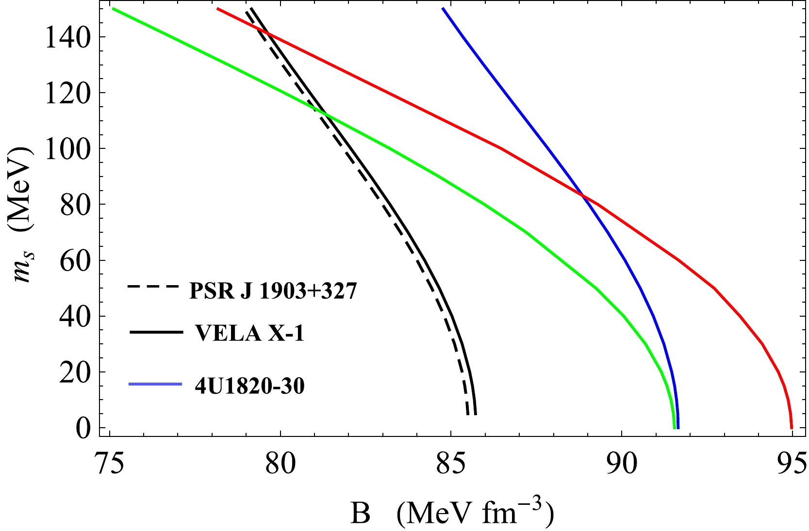
Figure 33. (color online) Plot of
$ m_{s} $ $\rm (MeV)$ with B ($\rm MeV fm^{-3}$ ) for three different stability regions. Stable region (below the green line), metastable region (between the green and red lines), and unstable region (above the red line).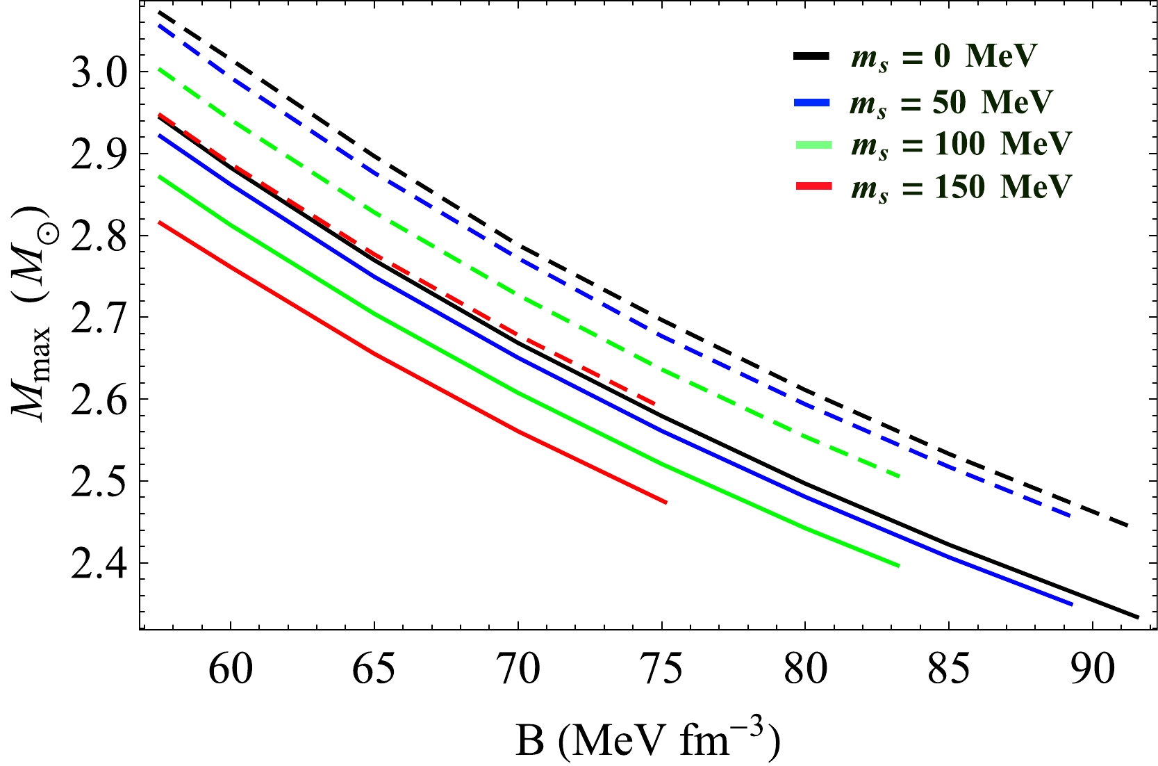
Figure 34. (color online) Variation in (
$M_{\rm max}(M_{\odot})$ ) with B for different values of$ m_{s}(=0, 50,100,150 $ MeV). Solid line for anisotropy parameter$ \alpha=0 $ , and dashed line for$ \alpha=0.3 $ .Star stability VELA X-1 4U 1820-30 PSR J1903+327 Stable $B > 81.34~\rm MeV/fm^{3}$ 

----- $B > 81~\rm MeV/fm^{3}$ 

$m_{s} < 112.4~\rm MeV$ 

----- $m_{s} < 114.1~\rm MeV$ 

Metastable $79.66<B(\rm MeV/fm^{3})<81.34$ 

$B > 88.88~\rm MeV/fm^{3}$ 

$79.32<B(\rm MeV/fm^{3})<81$ 

$112.4<m_{s}(\rm MeV)<141.45$ 

$m_{s} < 82.98~\rm MeV$ 

$114.1<m_{s}(\rm MeV)<143.5$ 

Unstable $B < 79.66~\rm MeV/fm^{3}$ 

$B < 88.88~\rm MeV/fm^{3}$ 

$B<79.32\; \rm MeV/fm^{3}$ 

$m_{s} > 141.45~\rm MeV$ 

$m_{s} > 82.98~\rm MeV$ 

$m_{s} > 143.5~\rm MeV$ 

Table 6. Comparative study of different stability windows for compact stars VELA X-1, 4U 1820-30, and PSR J 1903+327.
-
We would like to thank the referees for their useful comments.
Anisotropic strange quark star in Finch-Skea geometry and its maximum mass for non-zero strange quark mass (ms ≠ 0)
- Received Date: 2022-09-20
- Available Online: 2023-05-15
Abstract: A class of relativistic astrophysical compact objects is analyzed in the modified Finch-Skea geometry described by the MIT bag model equation of state of interior matter,


 DownLoad: