


 Abstract
 HTML
HTML Reference
 Related
 PDF
PDF


-
After the discovery of the Standard-Model-like (SM-like) Higgs boson at the Large Hadron Collider (LHC) [1, 2], the high-precision measurements of the properties of the SM-like Higgs boson are the most important tasks at the High-Luminosity LHC (HL-LHC) [3, 4] and future lepton colliders [5]. In other words, all Higgs productions and their decay channels should be probed as precisely as possible at future colliders. From these data, we can verify the SM in higher-energy regions and extract new physics. Among the Higgs decay channels,
$H\rightarrow Z \nu_l\bar{\nu}_l$ with$ l=e, \mu, \tau $ are of interest with regard to several aspects. First, if one considers$ Z\rightarrow \nu_l\bar{\nu}_l $ in the final state, the decay processes correspond to$ H\rightarrow $ invisible particles, which have recently studied at the LHC [6]. The search for invisible Higgs-boson decays play a key role in explaining the existence of dark matter. Furthermore, the decay channels contribute to the$ H\rightarrow $ lepton pair plus missing energy when the$ Z\rightarrow $ lepton pair is concerned in the final state. These contributions are also useful for precisely evaluating the SM backgrounds for the decay rates of the$ H\rightarrow $ lepton pair in the final state. For the above reasons, the precise decay rates for$ H\rightarrow Z \nu_l\bar{\nu}_l $ can provide an important tool for testing the SM at higher-energy scales and for probing new physics.One-loop contributions to
$ H\rightarrow Z \nu_l\bar{\nu}_l $ were computed in [7], and those for$ H\rightarrow 4 $ fermions were presented in [8–10]. In this study, we evaluate the one-loop contributions for the decay processes$ H\rightarrow Z \nu_l\bar{\nu}_l $ for$ l=e,\mu, \tau $ in the 't Hooft-Veltman gauge. In comparison with the previous calculations, we perform this computation with the following advantages. First, we focus on the analytical calculations for the decay channels and show a clear analytical structure for the one-loop amplitude of$ H\rightarrow Z \nu_l\bar{\nu}_l $ . As a result, we can explain and extract the dominant contributions to the decay widths when these are necessary (the dominant contributions are from Z-pole diagrams or the diagrams of$ H\rightarrow Z Z^* \rightarrow Z \nu_l\bar{\nu}_l $ in the decay channels, as we show in later sections). Furthermore, off-shell Higgs decays are valid in our work. In addition, one can generalize the couplings of Nambu-Goldstone bosons with Higgs bosons, gauge bosons, etc., as shown in our previous work [11]. We can easily extend our results beyond the Standard Model, as Nambu-Goldstone bosons play the same role as the changed Higgs in the extensions of the Standard Model Higgs sector. Last but not least, the signals of$ H\rightarrow Z \nu_l\bar{\nu}_l $ through Higgs productions at future lepton colliders are studied in our work. In further detail, one-loop form factors are expressed in terms of scalar one-loop Passarino-Veltman functions (called as PV-functions hereafter) in the standard notations of${\tt LoopTools}$ . As a result, one can evaluate the decay rates numerically by using the package. Moreover, the signals of$ H\rightarrow Z \nu_l\bar{\nu}_l $ through Higgs productions at future lepton colliders, for instance, the processes$ e^-e^+ \rightarrow ZH^* \rightarrow Z (Z \nu_l\bar{\nu}_l) $ with initial beam polarizations, are generated. The Standard Model backgrounds, such as$ e^-e^+ \rightarrow \nu_l\bar{\nu}_l ZZ $ , are also included in this analysis. In phenomenological results, we find that one-loop corrections make contributions of approximately 10% to the decay rates. These are sizeable contributions and should be taken into account at future colliders. We show that the signals$ H\rightarrow Z\nu_l\bar{\nu}_l $ are clearly visible at the center-of-mass energy$ \sqrt{s}=250 $ GeV and are difficult to probe in higher-energy regions owing to the dominant backgrounds.The remainder of this paper is organized as follows. In section II, we present the calculations for
$ H\rightarrow Z \nu_l\bar{\nu}_l $ in detail. We then show phenomenological results for the computations. The decay rates for on-shell and off-shell Higgs decay modes are studied, with the unpolarized and longitudinally polarized Z bosons in the final states. The signals of$ H\rightarrow Z \nu_l\bar{\nu}_l $ via the Higgs productions at future lepton colliders are also presented in this section. Conclusions are presented in section IV. In the appendies, we first summarize all the tensor reduction formulas for one-loop integrals that appear in this work. Numerical checks for the calculations are presented. All self-energy and counter-terms for the decay processes are presented in detail. One-loop Feynman diagrams in the 't Hooft-Veltman gauge for these decay channels are shown in Appendix E. -
We present the calculations for
$H(p_H)\rightarrow Z(q_1) \nu_l(q_2) \bar{\nu}_l(q_3)$ in detail. For these computations, we are working in the 't Hooft-Veltman gauge. Within the SM framework, all Feynman diagrams can be grouped into several classifications, as shown in Appendix E. In group$ G_0 $ , we have tree Feynman diagrams contributing to the decay processes. For group$ G_1 $ , we include all one-loop Feynman diagrams correcting to the vertex$ Z\nu_l\bar{\nu}_l $ . We then list all Z-pole Feynman diagrams in group$ G_2 $ and non Z-pole diagrams in group$ G_3 $ . The counterterm diagrams for this decay channels are classified into group$ G_4 $ .In general, the amplitude for
$ H(p_H)\rightarrow Z(q_1) \nu_l(q_2)\bar{\nu}_l(q_3) $ can be decomposed by the following Lorentz structure:$\begin{aligned}[b] {\cal{A}}_{H\rightarrow Z \nu_l\bar{\nu}_l} =& \Big\{ F_{00} g^{\mu \nu} + F_{12}\, q_1^\nu q_2^\mu + F_{13} \, q_1^\nu q_3^\mu \Big\} \\&\times\Big[ \bar{u} (q_2) \gamma_\nu P_L v (q_3) \Big] \varepsilon_\mu^* (q_1).\end{aligned} $

(1) Here,
$ F_{00} $ ,$ F_{12} $ , and$ F_{13} $ are form factors including both tree-level and one-loop diagram contributions. The form factors are functions of the Mandelstam invariants, such as$ s_{ij} = (q_i + q_j)^2 $ for$ i \neq j = 1,2,3 $ and mass-squared in one-loop diagrams. One also verifies that$ s_{12} + s_{13} + s_{23} = M_H^2 + M_Z^2 $ . In Eq. (1), projection operator$ P_L= (1-\gamma_5)/2 $ is taken into account, and the term$ \varepsilon_\mu^* (q_1) $ is the polarization vector of the final Z boson. Our computations can be summarized as follows. We first write the Feynman amplitude for all the diagrams mentioned above. By using${\tt Package-X}$ [12], all Dirac traces and Lorentz contractions in d dimensions are performed. The amplitudes are then casted into tensor one-loop integrals. The tensor integrals are next reduced to scalar PV-functions [13, 14]. All the relevant tensor reduction formulas are presented in Appendix A. The PV-functions can be evaluated numerically by using${\tt LoopTools}$ [15].All the form factors are calculated from Feynman diagrams in the 't Hooft-Veltman gauge, and their expressions are presented in this section. For the tree-level diagram, the form factor is given as
$ F_{00}^{(G_0)} (s_{12},s_{13},s_{23}) = \dfrac{2 \pi \alpha}{s_W^2 c_W^3} \dfrac{M_W}{s_{23}-M_Z^2 + {\rm i} \Gamma_Z M_Z}. $

(2) Here,
$ s_W (c_W) $ represents the sine (cosine) of the Weinberg angle, and$ \Gamma_Z $ represents the decay width of the Z boson.At the one-loop level, all form factors take form of
$ F_{ij} =\sum\limits_{G=\{G_1, \cdots, G_4\}}F_{ij}^{(G)} (s_{12},s_{13},s_{23}), ~ {\rm{for}}~ ij = \{00, 12, 13\}. $

(3) Here,
$\{G_1, G_2,\cdots, G_4\} = \{\text{group 1}, \text{group 2},\cdots, \text{group 4}\}$ correspond to the groups of Feynman diagrams in Appendix E. By considering each group of Feynman diagrams, analytical results for all the form factors are obtained, and they are presented in the following paragraphs. Taking the attribution from group$ G_1 $ , we have one-loop form factors accordingly:$ \begin{aligned}[b]\\[-22pt] F_{00}^{(G_1)} (s_{12},s_{13},s_{23}) =& -\dfrac{\alpha^2 }{8 s_W^4 c_W^5} \dfrac{M_W}{s_{23}-M_Z^2 + {\rm i} \Gamma_Z M_Z} \Big\{ -8 c_W^4 B_0(s_{23},M_W^2,M_W^2) -2 \big[c_W^2 (4 s_W^2-2) +1\big] B_0(s_{23},0,0) \\ & -8 c_W^4 \big[2 C_{00} -s_{23} (C_1 +C_2)\big](0,s_{23},0,0,M_W^2,M_W^2) -4 c_W^2 (2 s_W^2-1) \big[ M_W^2 C_0 +s_{23} C_2 -2 C_{00} \big] \\& \times (s_{23},0,0,0,0,M_W^2) + \big[ 4 C_{00} - 2 s_{23} C_2 -2 M_Z^2 C_0 \big] (s_{23},0,0,0,0,M_Z^2) +(2 c_W^2 + 1) \Big\},\\[-4pt] \end{aligned} $ 
(4) $ F_{ij}^{(G_1)} (s_{12},s_{13},s_{23}) = 0, \quad \text{for}\quad ij =\{12, 13\}. $

(5) For group
$ G_2 $ of the Feynman diagrams, the form factors can be divided into the fermion and boson parts as follows:$ F_{00}^{(G_2)} (s_{12},s_{13},s_{23}) = \dfrac{\alpha^2}{24\; s_W^4 c_W^7 M_W} \dfrac{1}{(s_{23}-M_Z^2 + {\rm i} \Gamma_Z M_Z)^2} \Big[ \sum\limits_{f} N_f^{C} F_{00, f}^{(G_2)} + F_{00, b}^{(G_2)} \Big]. $ 
(6) Here,
$ N_f^C $ represents the color number, which is 3 for quarks and 1 for leptons. For the fermion contributions, we take the top quark loop as an example. The analytical results are as follows:$ \begin{aligned}[b] F_{00, f}^{(G_2)} =& 2 c_W^2 M_W^2 \Big[ 8 s_W^2 (4 s_W^2-3)+9 \Big] \Big[ A_{0}(m_t^2) + s_{23} B_{1}(s_{23},m_t^2,m_t^2) - 2 B_{00}(s_{23},m_t^2,m_t^2) \Big] \\ & +2 m_t^2 c_W^2 \Big\{ 9 M_W^2 -2 c_W^2 (M_Z^2-s_{23}) \Big[4 s_W^2 (4 s_W^2-3)+9\Big] \Big\} B_{0}(s_{23},m_t^2,m_t^2) \\ & + m_t^2 c_W^4 (s_{23}-M_Z^2) \Big\{ 36 m_t^2+\Big[8 s_W^2 (4 s_W^2-3) +9\Big] (s_{12}+s_{13}) \Big\} C_{0}(M_Z^2,s_{23},M_H^2, m_t^2,m_t^2,m_t^2) \\& -m_t^2 c_W^4 (M_Z^2-s_{23}) \Big\{ (M_H^2+5 M_Z^2-s_{23}) \Big[8 s_W^2 (4 s_W^2-3)+9\Big] \\ & +8 s_W^2 (3-4 s_W^2) (s_{12}+s_{13}) \Big\} C_{1}(M_Z^2,s_{23},M_H^2, m_t^2,m_t^2,m_t^2) \\& -2 m_t^2 c_W^4 (M_Z^2-s_{23}) \Big\{ 9 M_H^2+ \Big[8 s_W^2 (4 s_W^2-3) +9\Big] (s_{12}+s_{13}) \Big\} C_{2}(M_Z^2,s_{23},M_H^2,m_t^2,m_t^2,m_t^2) \\& +8 m_t^2 c_W^4 (M_Z^2-s_{23}) \Big[8 s_W^2 (4 s_W^2-3)+9\Big] C_{00}(M_Z^2,s_{23},M_H^2,m_t^2,m_t^2,m_t^2). \end{aligned} $

(7) The contribution from the boson part is expressed as
$ \begin{aligned}[b] F_{00, b}^{(G_2)} =& 8 c_W^6 M_W^2 s_{23} -6 M_W^2 c_W^2 \Big[3 c_W^2 (4 c_W^2-1)+s_W^2\Big] A_{0}(M_W^2) -3 M_W^2 c_W^2 \Big[ A_{0}(M_Z^2) + A_{0}(M_H^2) \Big] \\ & +\dfrac{3}{2} c_W^4 M_H^2 (M_Z^2-s_{23}) B_{0}(M_H^2,M_Z^2,M_Z^2) + 12 M_W^2 s_W^4 c_W^4 (M_Z^2-s_{23}) B_{0}(M_Z^2,M_W^2,M_W^2) \\ & +3 c_W^4 (M_Z^2-s_{23}) \Big[ c_W^4 (M_H^2+24 M_W^2) -2 M_H^2 s_W^2 c_W^2 +M_H^2 s_W^4 \Big] B_{0}(M_H^2,M_W^2,M_W^2) \\&+12 M_W^2 c_W^2 \Big\{ (2 M_W^2 + 5 s_{23}) c_W^4 -2 M_W^2 s_W^4 \\ & +(M_Z^2-s_{23}) \Big[s_W^4-2 c_W^2 (c_W^2+1)\Big] c_W^2 \Big\} B_{0}(s_{23},M_W^2,M_W^2) \\ & +6 M_W^2 c_W^2 (M_Z^2-s_{23}) \Big[B_{0}(M_Z^2,M_H^2,M_Z^2) +B_{0}(s_{23},M_H^2,M_Z^2) \Big] -12 M_W^4 B_{0}(s_{23},M_H^2,M_Z^2) \\& -4 M_W^2 c_W^2 \Big[40 s_W^2 (4 s_W^2-3)+63\Big] B_{00}(s_{23},0,0) +12 M_W^2 c_W^2 B_{00}(s_{23},M_H^2,M_Z^2) \\& +12 M_W^2 c_W^2 \Big(9 c_W^4-2 s_W^2 c_W^2+s_W^4\Big) B_{00}(s_{23},M_W^2,M_W^2) + \dfrac{9}{2} c_W^4 M_H^2 (M_Z^2-s_{23}) B_{0}(M_H^2,M_H^2,M_H^2) \\& +2 M_W^2 c_W^2 s_{23} \Big[ 40 s_W^2 (4 s_W^2-3)+63 \Big] B_{1}(s_{23},0,0) + 24 c_W^6 M_W^2 s_{23} B_{1}(s_{23},M_W^2,M_W^2) \\ & -12 M_W^2 c_W^6 (M_Z^2-s_{23}) [ 4 M_Z^2+ c_W^2 (s_{12}+s_{13}) ] C_{1}(M_Z^2,s_{23},M_H^2,M_W^2,M_W^2,M_W^2) \\ & +24 M_W^2 c_W^6 (M_Z^2-s_{23}) (-c_W^2 M_H^2-s_{12}-s_{13}) C_{2}(M_Z^2,s_{23},M_H^2,M_W^2,M_W^2,M_W^2) \\ & -12 M_W^2 c_W^4 (M_Z^2-s_{23}) \Big\{ 2 c_W^4 \Big[ 2 M_W^2+5 M_Z^2 -2 (s_{12}+s_{13}) \Big] -(M_H^2+2 M_W^2) s_W^4 \\ & +s_W^2 c_W^2 \Big(M_H^2+2 M_W^2+s_{12}+s_{13}\Big) \Big\} C_{0}(M_Z^2,s_{23},M_H^2,M_W^2,M_W^2,M_W^2) \\& -12 c_W^4 (M_Z^2-s_{23}) \Big[ s_W^2 (s_W^2-2 c_W^2) (M_H^2+2 M_W^2) \\ & + (M_H^2+18 M_W^2) c_W^4 \Big] C_{00}(M_Z^2,s_{23},M_H^2,M_W^2,M_W^2,M_W^2) \\ & + 18 M_H^2 c_W^2 (s_{23}-M_Z^2) \Big[ -M_W^2 C_{0} + c_W^2 C_{00} \Big] (M_H^2,s_{23},M_Z^2,M_H^2,M_H^2,M_Z^2) \\ & + (M_Z^2-s_{23}) \Big[ 12 M_W^4 C_{0} -6 c_W^2 (M_H^2 c_W^2+2 M_W^2) C_{00} \Big] (M_Z^2,M_H^2,s_{23},M_H^2,M_Z^2,M_Z^2) . \end{aligned} $

(8) Other one-loop form factors follow the same convention:
$ F_{12}^{(G_2)} (s_{12},s_{13},s_{23}) = F_{13}^{(G_2)} (s_{13},s_{12},s_{23}) = - \dfrac{\alpha^2}{12 s_W^4 c_W^5 M_W} \dfrac{1}{s_{23}-M_Z^2 + {\rm i} \Gamma_Z M_Z} \Big[ \sum\limits_{f} N_f^{C} F_{12, f}^{(G_2)} + F_{12, b}^{(G_2)} \Big]. $

(9) Each part in the above equation has the form of (we take the top quark loop as an example for fermion contributions)
$ F_{12,f}^{(G_2)} = 9 m_t^2 c_W^2 C_{1}(M_Z^2,s_{23},M_H^2,m_t^2,m_t^2,m_t^2) + m_t^2 c_W^2 \Big[8 s_W^2 (4 s_W^2-3)+9\Big] \Big[ C_{0} + 4 \Big( C_{2} + C_{12} + C_{22} \Big) \Big] (M_Z^2,s_{23},M_H^2,m_t^2,m_t^2,m_t^2) $

(10) and
$ \begin{aligned}[b] F_{12,b}^{(G_2)} =& -12 c_W^2 M_W^2 \Big[ \big(5 c_W^4-2 c_W^2 s_W^2+s_W^4\big) C_{0} + C_{1} \Big] (M_Z^2,s_{23},M_H^2,M_W^2,M_W^2,M_W^2) \\ & +3 c_W^2 M_H^2 \Big[ C_{12}(M_Z^2,M_H^2,s_{23},M_H^2,M_Z^2,M_Z^2) -3 \Big( C_{1} + C_{11} + C_{12} \Big) (M_H^2,s_{23},M_Z^2,M_H^2,M_H^2,M_Z^2) \Big] \\& +6 M_W^2 \Big[ C_{1} + C_{2} + C_{12} \Big] (M_Z^2,M_H^2,s_{23},M_H^2,M_Z^2,M_Z^2) -6 c_W^2 \Big[ s_W^2 (s_W^2 - 2 c_W^2) (M_H^2+2 M_W^2) + c_W^4 (M_H^2+18 M_W^2) \Big] \\& \times \Big[ C_{2} + C_{12} + C_{22} \Big] (M_Z^2,s_{23},M_H^2,M_W^2,M_W^2,M_W^2) . \end{aligned} $

(11) We change to the contributions of all Feynman diagrams in group
$ G_3 $ . For this group, there are no Z-pole diagrams including in one-loop form factors. However, we have one-loop box diagrams. There are a triple gauge boson vertex and the propagator of leptons or two propagators of leptons in one-loop box diagrams; hence, we have tensor box integrals, for which the highest rank is$ R=2 $ in the amplitude. It is explained that the corresponding form factors are expressed in terms of the PV-functions C- and up to$ D_{33} $ -coefficients.$ \begin{aligned}[b] F_{00}^{(G_3)} =& \dfrac{\alpha^2 M_W}{4 s_W^4 c_W^5} \Bigg\{ 2 c_W^4 \Big[ (2 s_W^2-1) C_{0}(M_Z^2,0,s_{13},0,0,M_W^2) + (3 c_W^2+1) C_{0}(0,s_{23},0,0,M_W^2,M_W^2) \\& + C_{2}(0,M_H^2,s_{13},0,M_W^2,M_W^2) + C_{2}(0,M_H^2,s_{12},0,M_W^2,M_W^2) \Big] +C_{0}(M_Z^2,0,s_{13},0,0,M_Z^2) \\ &+C_{2}(0,M_H^2,s_{13},0,M_Z^2,M_Z^2) +C_{2}(0,M_H^2,s_{12},0,M_Z^2,M_Z^2) +8 c_W^6 \Big[ D_{00}(s_{12},M_Z^2,s_{23},0,0, M_H^2,0,M_W^2,M_W^2,M_W^2) \\ & + D_{00}(s_{13},M_Z^2,s_{23},0,0, M_H^2,0,M_W^2,M_W^2,M_W^2) \Big] - 2 c_W^6 \Big[ (2 M_Z^2+s_{12}) D_{1}(s_{12},M_Z^2,s_{23},0,0, M_H^2,0,M_W^2,M_W^2,M_W^2) \\ & + (2 M_Z^2+s_{13}) D_{1}(s_{13},M_Z^2,s_{23},0,0, M_H^2,0,M_W^2,M_W^2,M_W^2) \Big] \\ &+ c_W^4 \Big\{ \Big[2 c_W^2 (3 M_H^2-2 s_{23}-3 s_{13}) +s_W^2 (s_{13}-M_H^2) \Big] D_{3}(s_{13},M_Z^2,s_{23}, 0,0,M_H^2,0,M_W^2,M_W^2,M_W^2) \\ & + \Big[ s_W^2 (s_{12} - M_H^2) + 2 c_W^2 (3 M_H^2 - 2 s_{23} - 3 s_{12}) \Big] D_{3}(s_{12},M_Z^2,s_{23},0,0, M_H^2,0,M_W^2,M_W^2,M_W^2) \Big\} \\ & +c_W^4 (3 c_W^2+1) \Big[ (M_W^2-s_{12}) D_{0}(s_{12},M_Z^2,s_{23},0,0, M_H^2,0,M_W^2,M_W^2,M_W^2) \\ & + (M_W^2-s_{13}) D_{0}(s_{13},M_Z^2,s_{23},0,0, M_H^2,0,M_W^2,M_W^2,M_W^2) \Big] \\ & +(s_{12}-M_Z^2) \Big[2 c_W^4 (1-2 s_W^2) D_{2}(M_Z^2,s_{12},M_H^2, s_{13},0,0,0,0,M_W^2,M_W^2) -D_{2}(M_Z^2,s_{12},M_H^2, s_{13},0,0,0,0,M_Z^2,M_Z^2) \Big] \\ & +s_W^2 c_W^4 \Big[ (M_Z^2-s_{13}) D_{2}(s_{13},M_Z^2,s_{23},0,0, M_H^2,0,M_W^2,M_W^2,M_W^2) + (M_Z^2 - s_{12}) D_{2}(s_{12},M_Z^2,s_{23},0,0, M_H^2,0,M_W^2,M_W^2,M_W^2) \Big] \\ & +(s_{23}+s_{12}) \Big[ 2 c_W^4 (2 s_W^2-1) D_{3}(M_Z^2,s_{12},M_H^2, s_{13},0,0,0,0,M_W^2,M_W^2) +D_{3}(M_Z^2,s_{12},M_H^2, s_{13},0,0,0,0,M_Z^2,M_Z^2) \Big] \\ & + \Big[M_Z^2 D_{0} + s_{12} D_{1} -2 D_{00}\Big] (M_Z^2,s_{12},M_H^2, s_{13},0,0,0,0,M_Z^2,M_Z^2) \\ & + 2 c_W^4 (1-2 s_W^2) \Big[ 2 D_{00} - s_{12} D_{1} - M_W^2 D_{0} \Big] (M_Z^2,s_{12},M_H^2, s_{13},0,0,0,0,M_W^2,M_W^2) \Bigg\} . \end{aligned} $

(12) In addition, we have other form factors, which are expressed as follows:
$ \begin{aligned}[b] F_{12}^{(G_3)} = &\dfrac{\alpha^2 M_W}{2 s_W^4 c_W^5} \Bigg\{ \Big[ D_{2} +D_{12} +D_{23} \Big] (M_Z^2,s_{12},M_H^2, s_{13},0,0,0,0,M_Z^2,M_Z^2) \\& -4 c_W^6 \Big[ D_{3} + D_{13} \Big](s_{13},M_Z^2, s_{23},0,0,M_H^2,0,M_W^2,M_W^2,M_W^2) \\&-2 c_W^4 (1- 2 s_W^2) \Big[ D_{2} + D_{12} + D_{23} \Big] (M_Z^2,s_{12},M_H^2,s_{13}, 0,0,0,0,M_W^2,M_W^2) \\ & +2 c_W^4 \Big[ 2 c_W^2 \Big( D_{11} + D_{12} \Big) +(s_W^2 - c_W^2) D_{2} \Big] (s_{12},M_Z^2,s_{23},0,0, M_H^2,0,M_W^2,M_W^2,M_W^2) \Bigg\} , \end{aligned} $

(13) $ \begin{aligned}[b] F_{13}^{(G_3)} =& \dfrac{\alpha^2 M_W}{2 s_W^4 c_W^5} \Bigg\{ -\Big[ D_{13} + D_{33} \Big] (M_Z^2,s_{12},M_H^2, s_{13},0,0,0,0,M_Z^2,M_Z^2)\\& -4 c_W^6 \Big[ D_{3} + D_{13} \Big] (s_{12},M_Z^2,s_{23},0,0, M_H^2,0,M_W^2,M_W^2,M_W^2) \\ & +2 c_W^4 (1-2 s_W^2) \Big[ D_{13} + D_{33} \Big] (M_Z^2,s_{12},M_H^2,s_{13}, 0,0,0,0,M_W^2,M_W^2) \\ & + 2 c_W^4 \Big[ 2 c_W^2 \Big( D_{11} + D_{12} \Big) + \big(s_W^2 - c_W^2\big) D_{2} \Big] (s_{13},M_Z^2,s_{23},0,0, M_H^2,0,M_W^2,M_W^2,M_W^2) \Bigg\} . \end{aligned}$

(14) It is stress that one has the following relation:
$ F_{12}^{(G_3)}(s_{12},s_{13},s_{23}) = F_{13}^{(G_3)}(s_{13},s_{12},s_{23}). $

(15) If we apply several transformations for box-functions, we can confirm the relation. The transformations for box-functions are not presented in this subsection. Instead, we verify the relation via numerical checks. One finds that two representations for
$ F_{13}^{(G_3)} $ in Eqs. (14) and (16) agree well up to the last digit at several sampling points.With all the form factors, the decay rates can be evaluated as follows:
$ \begin{aligned}[b] \Gamma_{H\rightarrow Z\nu_l \bar{\nu_l}} =& \dfrac{1}{256 \pi^3 M_H^3 M_Z^2} \int \limits_{4 m_{\nu_l}^2}^{(M_H-M_Z)^2} {\rm d} s_{23} \int \limits_{s_{12}^{\text{min}}}^{s_{12}^{\text{max}}} {\rm d} s_{12} \; \Bigg\{ \Big(M_Z^2 (2 s_{23}-M_H^2) + s_{12} s_{13}\Big) \Big[ \Big|F_{00}^{(G_0)} \Big|^2 + 2\,{\cal{R}}\text{e} \Big( F_{00}^{(G_0),*}\cdot \sum\limits_{i=1}^4 F_{00}^{(G_i)} \Big) \Big] \\&+ \Big(M_H^2 M_Z^2 - s_{12} s_{13}\Big) \Big[ \Big(M_Z^2-s_{12}\Big) {\cal{R}}\text{e} \Big( F_{00}^{(G_0),*}\cdot \sum\limits_{i=1}^4 F_{12}^{(G_i)} \Big) + \big( s_{12} \leftrightarrow s_{13} \big) \Big] \Bigg\} . \end{aligned} $ 
(16) Here,
$ s_{12}^{\text{max},\text{min}} = \dfrac{1}{2} \Bigg\{ M_H^2 + M_Z^2 - s_{23} \pm \sqrt{ \Big(M_H^2 + M_Z^2 - s_{23}\Big)^2 - 4 M_H^2 M_Z^2 } \Bigg\} . $

(17) The polarized Z boson case is considered next. The longitudinal polarization vectors for Z bosons are defined in the rest frame of the Higgs boson:
$ \varepsilon_{\mu}(q_1, \lambda=0) = \dfrac{4 M_{H^*}^2 \; q_{1, \mu} - (s_{23}+M_Z^2)\; p_{H,\mu} } {M_Z \sqrt{\lambda(s_{23},4M_{H^*}^2,M_Z^2) }}. $

(18) Here, the off-shell Higgs mass is given by
$ p_H^2=M_{H^*}^2 \neq M_H^2 $ . The Kallën function is defined as$ \lambda (x, y, z) = (x - y - z)^2 - 4 yz $ . We then arrive at$ \begin{aligned}[b] \Gamma_{H\rightarrow Z_L \nu_l \bar{\nu_l}} = \dfrac{1}{256 \pi^3 M_{H^*}^3 M_Z^2} \int \limits_{4 m_{\nu_l}^2}^{(M_{H^*}-M_Z)^2} {\rm d} s_{23} \int \limits_{s_{12}^{\text{min}}} ^{s_{12}^{\text{max}}}{\rm d} s_{12} \dfrac{ \Big(s_{23}-4 M_{H^*}^2+M_Z^2\Big) \Big(s_{12} s_{13}-M_Z^2 M_{H^*}^2\Big) } {[s_{23}-M_Z^2 -4 M_{H^*}^2]^2- 16 M_Z^2 M_{H^*}^2 } \end{aligned} $

$ \begin{aligned}[b] \quad & \times \; \Bigg\{ \Big(s_{23}-4 M_{H^*}^2+M_Z^2\Big) \Big[ \Big|F_{00}^{(G_0)}\Big|^2 + 2\, {\cal{R}}\text{e} \Big( F_{00}^{(G_0),*} \times \sum\limits_{i=1}^4 F_{00}^{(G_i)} \Big) \Big] \\& + \Big[ \Big( s_{23}^2 - M_Z^4 + 4 M_{H^*}^2 M_Z^2 \Big) + \Big( s_{23} -4 M_{H^*}^2 + M_Z^2 \Big)s_{12} \Big] \times{\cal{R}}\text{e} \Big( F_{00}^{(G_0),*} \sum\limits_{i=1}^4 F_{12}^{(G_i)} \Big) + \big(s_{12} \leftrightarrow s_{13} \big) \Bigg\} . \end{aligned} $

(19) Here,
$ s_{12}^{\text{min, max}} $ are obtained as in Eq. (17), in which$ M_H $ is replaced with the off-shell Higgs mass$ M_{H^*} $ .In the next section, we present phenomenological results for the decay processes. Before generating the data, numerical checks for the calculations are performed. The
$ UV $ - finiteness and$ \mu^2 $ -independence of the results are verified. Numerical results for these checks are presented in Appendix B. One finds that the results have good stability over 14 digits. -
For the phenomenological results, we use the following input parameters:
$ M_Z = 91.1876 $ GeV,$ \Gamma_Z = 2.4952 $ GeV,$ M_W = 80.379 $ GeV,$ \Gamma_W = 2.085 $ GeV,$ M_H =125.1 $ GeV, and$ \Gamma_H =4.07\cdot 10^{-3} $ GeV. The lepton masses are given as$ m_e =0.00052 $ GeV,$ m_{\mu}=0.10566 $ GeV, and$ m_{\tau} = 1.77686 $ GeV. The quark masses are$ m_u= 0.00216 $ GeV,$ m_d= 0.0048 $ GeV,$ m_c=1.27 $ GeV,$ m_s = 0.93 $ GeV,$ m_t= 173.0 $ GeV, and$ m_b= 4.18 $ GeV. We work in the so-called$ G_{\mu} $ -scheme, in which the Fermi constant is taken as$ G_{\mu}=1.16638\cdot 10^{-5} $ GeV$ ^{-2} $ and the electroweak coupling can be calculated appropriately as follows:$ \alpha = \sqrt{2}/\pi G_{\mu} M_W^2(1-M_W^2/M_Z^2) = 1/132.184. $

(20) We present the phenomenological results in the following subsections. We first discuss the decay rates for the on-shell Higgs decay
$ H\rightarrow Z \nu_l\bar{\nu}_l $ . In Table 1, the decay rates for on-shell Higgs decay to$ Z \nu_e\bar{\nu}_e $ are presented. In the first column, the cuts for the invariant mass of the final neutrino-pair are applied. The decay rates for the unpolarized case of the final Z boson are presented in the second column. The results in the last column are the decay rates corresponding to the longitudinal polarization of the final Z boson. Furthermore, in this table, the result for the tree level (full one-loop) decay width is presented on the first (second) line. When we consider all generation of neutrinos, one should add to data by overall factor 3. The one-loop corrections make contributions of ~10% to the tree-level decay rates. We note that one-loop corrections are evaluated as follows:$ m_{\nu_e\bar{\nu}_e}^{\rm{cut}} $ /GeV

$ \Gamma_{H\rightarrow Z \nu_e\bar{\nu}_e} $ /keV

$ \Gamma_{H\rightarrow Z_{L} \nu_e\bar{\nu}_e} $ /keV

0 5.8177 2.2872 6.4174 2.5061 5 5.7014 2.1736 6.2902 2.3818 10 5.3401 1.8515 5.8943 2.0293 20 3.7362 0.8389 4.1305 0.9201 Table 1. Decay rates for on-shell Higgs decay into
$ Z \nu_e\bar{\nu}_e $ . The first (second) line corresponds to the tree level (full one-loop) decay width.$ \delta [\%] = \dfrac{\Gamma^{\text{Full}} -\Gamma^{\text{Tree}} }{\Gamma^{\text{Tree}}} \times 100{\text%}. $

(21) We next consider the off-shell Higgs decay to
$ Z \nu_e\bar{\nu}_e $ . The numerical results are presented in Table 2. In this case, we only consider the unpolarized Z boson in the final state. In the first column, the off-shell Higgs mass$ M_{H^*} $ is shown in the range of 200 to 500 GeV. The off-shell decay widths are presented in the second column, where the first (second) line is for the tree-level (full one-loop) decay rate. It is worth mentioning that the results for the off-shell Higgs decays agree well with the decay rates in [16]. This indicates that the main contributions to the decay rates are from the values around the peak of the Z-pole decay to$ \nu_l\bar{\nu}_l $ (this explanation will be confirmed later).$ M_{H^*} $ /GeV

$ \Gamma_{H\rightarrow Z \nu_e\bar{\nu}_e} $ /GeV

200 0.0478 0.0541 300 0.3383 0.3789 400 1.0124 1.1418 500 2.2101 2.4865 Table 2. Decay rates for off-shell Higgs decay into
$ Z \nu_e\bar{\nu}_e $ . The first (second) line corresponds to the tree level (full one-loop) decay width.For the experimental analyses, differential decay rates with respect to the invariant mass of the neutrino-pair are of interest. These correspond to the decay rates of Higgs decay to Z plus missing energy. Thus, the data provide the precise backgrounds for the signals of Higgs decay to the lepton-pair when the
$ Z\rightarrow $ lepton-pair is taken into account. This also contributes to the signals of$ H\rightarrow $ invisible particles if the decay of the final Z boson to the neutrino-pair is considered. In Fig. 1, we show for the differential decay rates with respect to$ m_{\nu_l\bar{\nu}_l} $ for the case of the unpolarized Z final state. We apply a cut of$ m_{\nu_l \bar{\nu}_l}^{\text{cut}} \ge 5 $ GeV for this study. In the left panel, the triangle points are for the tree-level decay widths, and the rectangle points are for the full one-loop decay widths. In the right panel, the electroweak corrections are plotted. One finds that the corrections make contributions in the range of 9.4% to 10.8%. In Fig. 2, the same distributions are shown in the longitudinal polarization of the final Z boson. We use the same convention as the previous case. We find that the corrections make contributions in the range of 9.4% to 9.8%.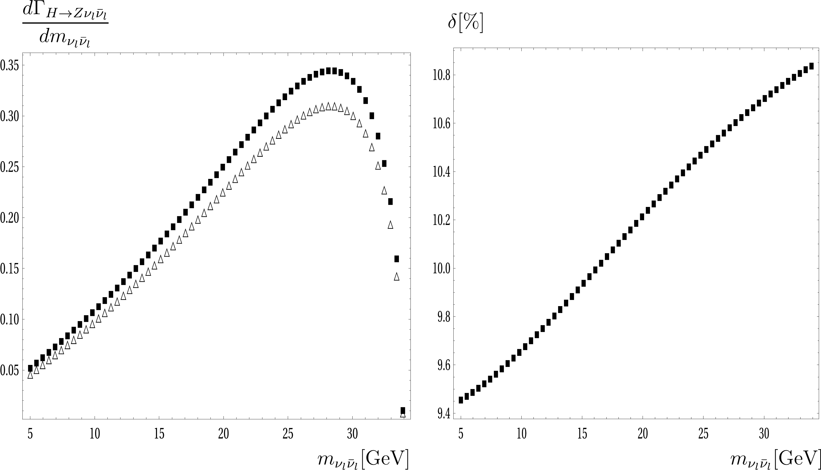
Figure 1. Differential decay rates (left panel) and corrections (right panel) with respect to
$ m_{\nu_l\bar{\nu}_l} $ for the unpolarized Z boson case. In the left panel, the triangle points are for the tree-level decay widths, and the rectangle points are for the full one-loop decay widths. In the right panel, the electroweak corrections are shown as the rectangle points.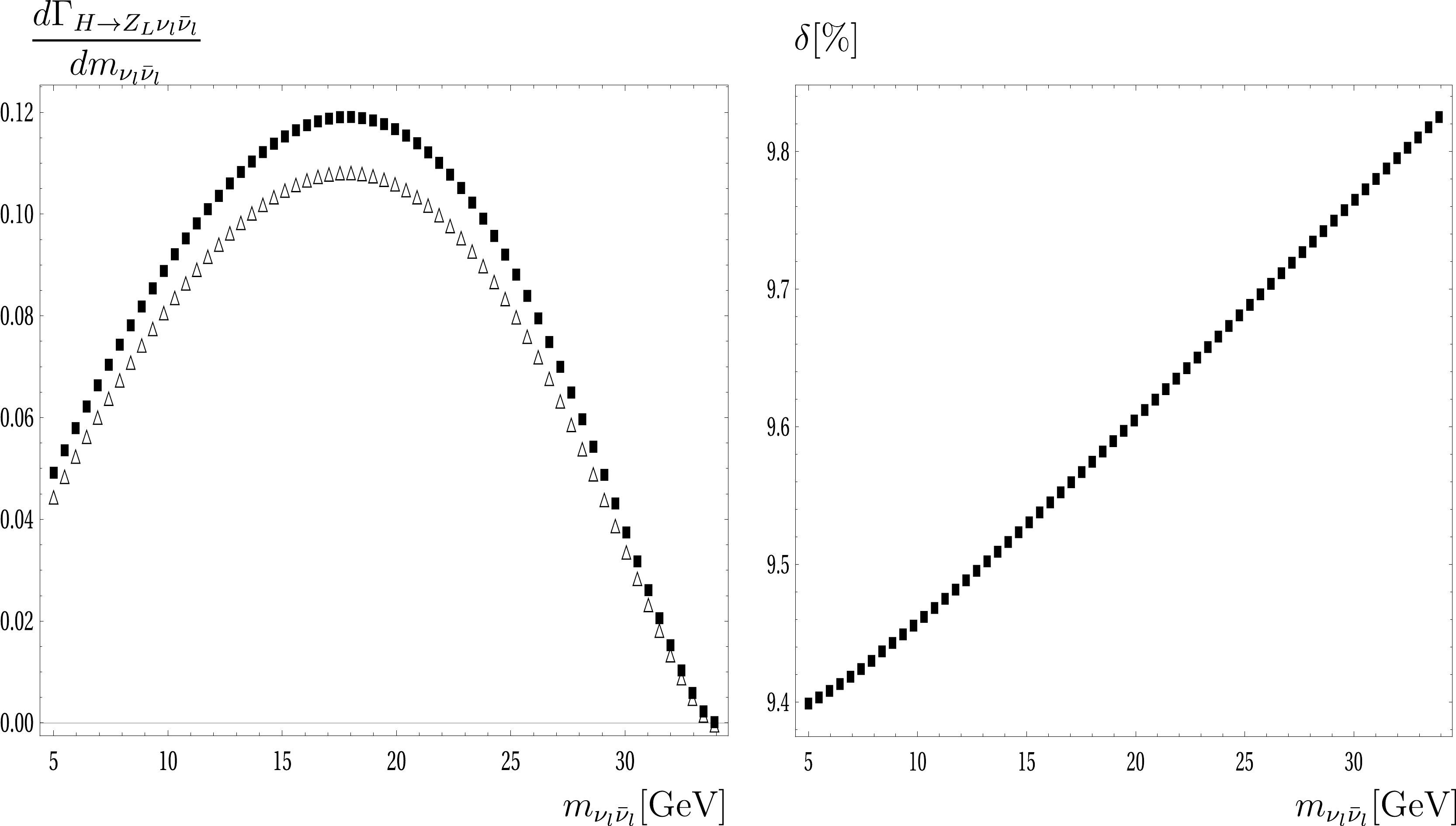
Figure 2. Differential decay rates (left panel) and corrections (right panel) with respect to
$ m_{\nu_l\bar{\nu}_l} $ in the longitudinal polarization case for the Z boson. In the left panel, the triangle points are for the tree-level decay widths, and the rectangle points are for the full one-loop decay widths. In the right panel, the electroweak corrections are plotted as the rectangle points.The differential decay rates with respect to
$ m_{\nu_l\bar{\nu}_l} $ for the off-shell Higgs case at$ M_{H}^* =500 $ GeV are presented. In Fig. 3, we observe a peak at$ m_{\nu_l\bar{\nu}_l} = M_Z $ , which corresponds to$ Z\rightarrow \nu_l\bar{\nu}_l $ . The decay rates exhibit high values around the peak and decrease rapidly beyond the peak. The corrections are from 10% to 25% throughout the range of$ m_{\nu_l\bar{\nu}_l} $ . We note that a cut of$ m_{\nu_l\bar{\nu}_l}^{\text{cut}} \ge 5 $ GeV is employed in the distribution. From the distribution, the main contributions to the off-shell Higgs decay rates come from the corresponding values around the Z-peak, indicating that the off-shell Higgs decay rates in this work agree well with the results in [16]. This supports the previous conclusion regarding the data in Table 2. Additionally, for the entire range of the Higgs mass, we check numerically that the dominant contributions to the decay rates come from the Z-pole diagrams or the diagrams of$H\rightarrow Z Z^* \rightarrow Z \nu_l\bar{\nu}_l$ (from groups 1 and 2) in these decay channels. The same conclusion was drawn in [17].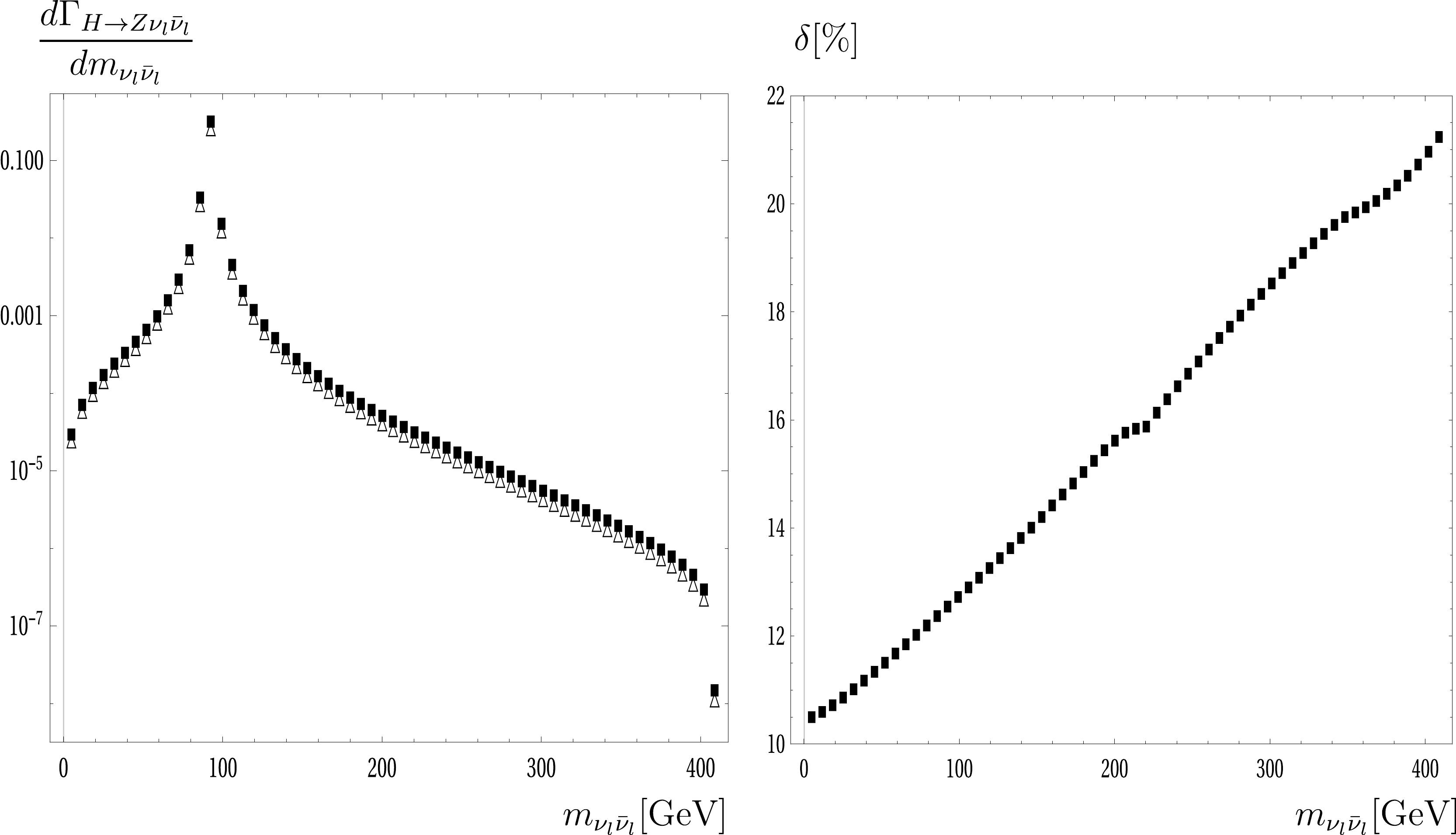
Figure 3. Differential decay rates (left panel) and corrections (right panel) with respect to
$ m_{\nu_l\bar{\nu}_l} $ for the off-shell Higgs case. In the left panel, tree-level decay widths are plotted as triangle points, and full one-loop decay widths are shown as rectangle points. In the right panel, the electroweak corrections are presented as the rectangle points.We turn our attention to analyze the signals
$ H\rightarrow Z \nu_l\bar{\nu}_l $ through Higgs productions at future lepton colliders, such as$ e^-e^+ \rightarrow ZH^* \rightarrow Z (Z \nu_l\bar{\nu}_l) $ , with the initial beam polarizations. The differential cross section with resprect to$ M_{H^*} $ is given as [16]$\begin{aligned}[b]& \dfrac{{\rm d}\sigma^{e^-e^+\rightarrow ZH^*\rightarrow Z(Z \nu_l\bar{\nu}_l)} (\sqrt{s}) }{{\rm d} M_{H^*}} \\=&(2M_{H^*}^2) \dfrac{ \sigma^{e^-e^+\rightarrow ZH^*}(\sqrt{s}, M_{H^*})} {[(M_{H^*}^2-M_H^2)^2+ \Gamma_H^2 M_H^2 ]}\\&\times \dfrac{\Gamma_{H^*\rightarrow ZZ} (M_{H^*})}{\pi}. \end{aligned}$

(22) The Feynman diagram is shown in Fig. 4. The cross section for
$ e^-e^+ \rightarrow ZH^* $ can be found in [16]. The total cross section for these processes can be computed as follows: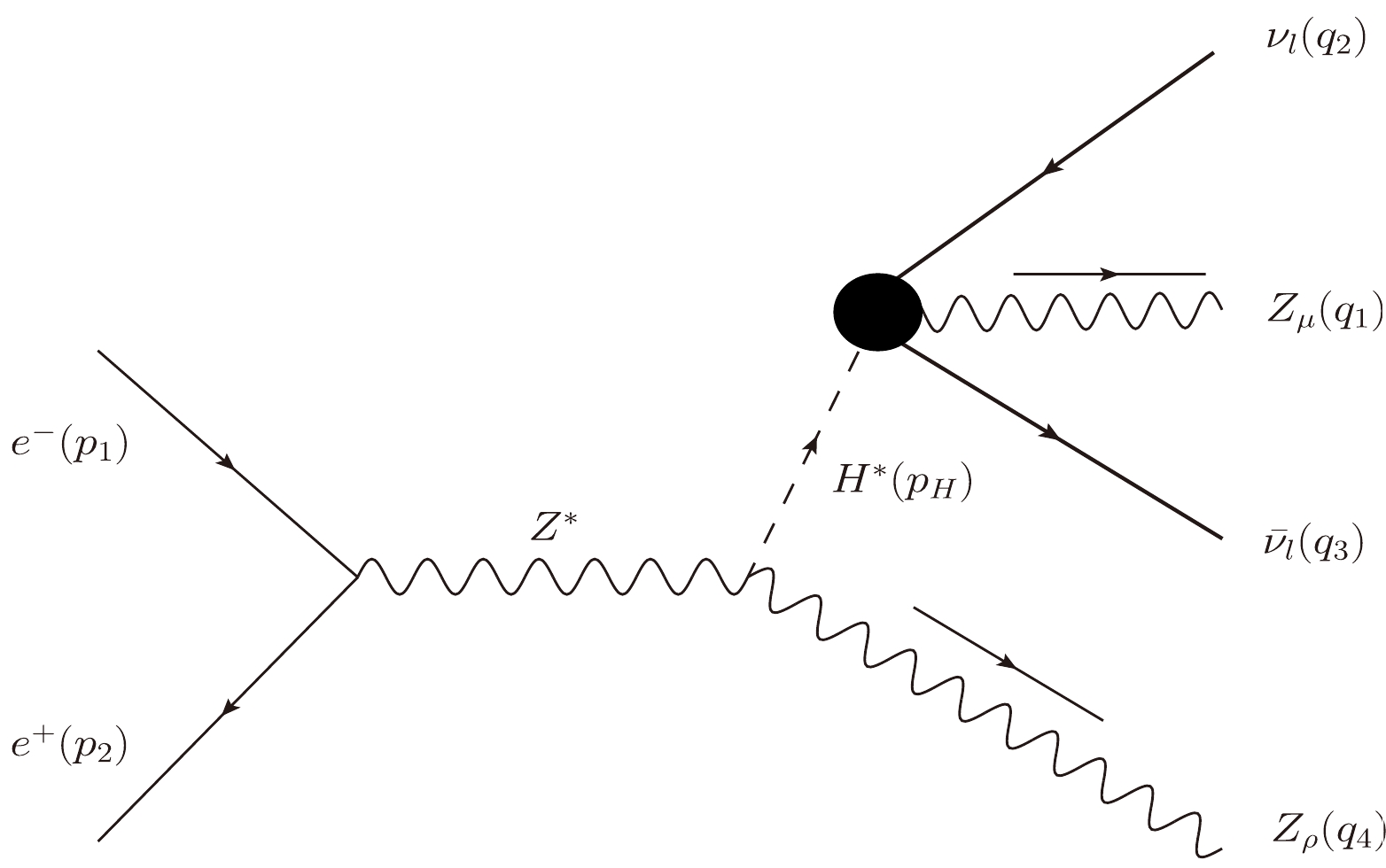
Figure 4. Feynman diagram for the processes
$ e^-e^+ \rightarrow Z(Z\nu_l\bar{\nu_l}) $ at the ILC with the blob representing one-loop corrections to$ H\rightarrow Z\nu_l\bar{\nu_l} $ .$ \sigma^{e^-e^+\rightarrow ZH^*\rightarrow Z(Z \nu_l\bar{\nu}_l)} = \int\limits_{M_Z}^{\sqrt{s}-M_Z} {\rm d} M_{H^*} \; \dfrac{{\rm d}\sigma^{e^-e^+\rightarrow ZH^*\rightarrow Z(Z \nu_l\bar{\nu}_l)} (\sqrt{s}) }{{\rm d} M_{H^*}}. $

(23) In Table 3, we present the cross sections for the signals of Higgs decay to
$ Z \nu_l\bar{\nu}_l $ via$ e^-e^+ \rightarrow ZH^* \rightarrow Z (Z \nu_l\bar{\nu}_l) $ with the initial beam polarizations (taking all three generations of neutrinos in the data). The second (third) column corresponds to the signals at tree level (full correction) cross sections. The last column is for the SM backgrounds, which are the tree level of the reactions$ e^-e^+ \rightarrow Z Z \nu_l\bar{\nu}_l $ . The background processes are generated by using GRACE [18]. For each center-of-mass energy, the first line corresponds to the LR case, and the second line corresponds to the RL polarization case. We show that the signals$ H\rightarrow Z\nu_l\bar{\nu}_l $ can be probed at the center-of-mass energy$ \sqrt{s}=250 $ GeV and that they are difficult to measure in higher-energy regions owing to the dominant backgrounds.$\sqrt{s} /{\rm{GeV} }$ 

$\sigma_{\text{sig} }^{\text{Tree} }/{\rm{fb} }$ 

$\sigma_{\text{sig} }^{\text{Full} }/{\rm{fb} }$ 

$\sigma_{\text{bkg} }/{\rm{fb} }$ 

250 2.43873 2.69398 0.00309 1.58487 1.74649 0.00016 500 0.68498 0.75668 16.7839 0.44404 0.48932 1.33409 1000 0.26879 0.29692 164.146 0.17424 0.19201 1.16635 Table 3. Total cross section of
$ e^-e^+ \rightarrow Z(Z\nu_l\bar{\nu_l}) $ . The first line presents results for the$ LR $ of$ e^-e^+ $ , and the second line presents results for the$ RL $ of$ e^-e^+ $ . Tree generations for neutrinos are taken into the results.In Fig. 5, we plot the distributions for the cross section as functions of
$ M_{H^*} $ at the center-of-mass energy of$ \sqrt{s}=500 $ GeV, considering the initial polarization cases for$ e^-e^+ $ . Cross sections for the LR and RL cases are shown in the left and right panels, respectively. For the signal cross sections, tree-level cross sections are plotted as dashed lines, and full one-loop cross sections are presented as solid lines. The SM backgrounds are shown as dotted points. The off-shell Higgs mass$ M_{H^*} $ is varied from$ M_Z $ to$ \sqrt{s}-M_Z $ . It is observed that the cross sections are dominant around the on-shell Higgs mass$ M_{H^*}\sim 125 $ GeV. It is well-known that we have another peak that is around the ZH threshold ($ \sim M_Z+M_H= 215 $ GeV). Owing to the small value of the total decay width of the Higgs boson, the on-shell Higgs mass peak becomes more visible than the later one. In the off-shell Higgs mass region, the cross sections are far smaller (by approximately 2 orders of magnitude) than those around the on-shell Higgs mass peak. We observe that the signals are clearly visible at the on-shell Higgs mass$ M_{H^*}=125 $ GeV. In the off-shell Higgs mass region, the SM backgrounds are far larger than the signals. These large contributions are mainly attributed to the dominant of t-channel diagrams appear in the background processes.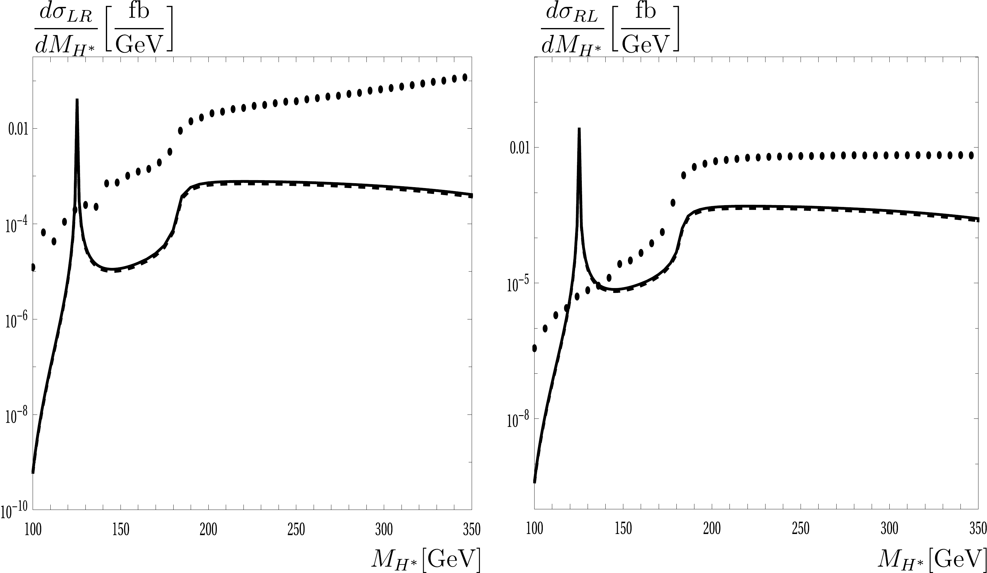
Figure 5. Off-shell Higgs decay rates as a function of
$ M_{H^*} $ at the center-of-mass energy of$ \sqrt{s}=500 $ GeV. Three generations for neutrinos are included in the results. Cross sections for the LR and RL cases are shown in the left and right panels, respectively. For the signal cross sections, tree-level cross sections are shown as dashed lines, and full one-loop cross sections are shown as solid lines. The dotted points indicate the SM backgrounds.Full one-loop electroweak corrections to the process
$ e^-e^+ \rightarrow ZH $ and the SM background processes with the initial beam polarizations should be taken into account for the above analyses. The corrections can be generated by using the program [18], and they were recently studied in [19]. Furthermore, by generalizing the couplings of Nambu-Goldstone bosons to Higgs bosons, gauge bosons, etc., as in [11], we can extend our work beyond the SM. These topics will be addressed in our future works. -
Analytical results for one-loop contributions to the decay processes
$ H\rightarrow Z \nu_l\bar{\nu}_l $ for$ l=e,\mu, \tau $ in the 't Hooft-Veltman gauge were presented. The calculations were performed within the Standard Model framework. One-loop form factors are expressed in terms of the Passarino-Veltman functions in the standard conventions of${\tt LoopTools}$ , for which the decay rates can be evaluated numerically. We also studied the signals of$ H\rightarrow Z \nu_l\bar{\nu}_l $ through Higgs productions at future lepton colliders, such as$e^-e^+ \rightarrow ZH^* \rightarrow Z (Z \nu_l\bar{\nu}_l)$ , with the initial beam polarizations. The SM background processes for this analysis were taken into account. Phenomenological results indicated that one-loop corrections make contributions of approximately 10% to the decay rates. These are sizeable contributions and should be taken into account at future colliders. We show that the signals$ H\rightarrow Z\nu_l\bar{\nu}_l $ are clearly visible at the center-of-mass energy$ \sqrt{s}=250 $ GeV and are difficult to probe in higher-energy regions owing to the dominant backgrounds. -
We present all the tensor one-loop reduction formulas applied for this calculation in this appendix. The technique is based on the method in [13]. Tensor one-loop one-, two-, three-, and four-point integrals with rank R are defined as follows:
$\begin{aligned}[b]& \{A; B; C; D\}^{\mu_1\mu_2\cdots \mu_R}\\ =& (\mu^2)^{2-d/2} \int \frac{{\rm d}^dk}{(2\pi)^d} \dfrac{k^{\mu_1}k^{\mu_2} \cdots k^{\mu_R}}{\{P_1; P_1 P_2;P_1P_2P_3; P_1P_2P_3P_4\}}.\end{aligned} \tag{A1}$

Here, the inverse Feynman propagators
$ P_j $ ($j=1,2,\cdots, 4$ ) are given by$ P_j = (k+ q_j)^2 -m_j^2 +{\rm i}\rho. \tag{A2}$

In this definition, the momenta
$ q_j = \sum\limits_{i=1}^j p_i $ with$ p_i $ for the external momenta are taken into account, and$ m_j $ denotes the internal masses in the loops. The internal masses can be real and complex in the calculation. Following the dimensional regularization method, one-loop integrals are peformed in space-time dimension$ d=4-2\varepsilon $ . The renormalization scale is introduced as$ \mu^2 $ in this definition, which helps to track the correct dimension of the integrals in space-time dimension d. If the numerators of one-loop integrands in Eq. (A1) are 1, we have the corresponding scalar one-loop functions (denoted as$ A_0 $ ,$ B_0 $ ,$ C_0 $ , and$ D_0 $ ). All the reduction formulas for one-loop tensor integrals up to rank$ R=3 $ are presented in the following paragraphs. In detail, we have the following reduction expressions for one-loop two-point tensor integrals:$ A^{\mu} = 0, \tag{A3}$

$ A^{\mu\nu} = g^{\mu\nu} A_{00}, \tag{A4}$

$ A^{\mu\nu\rho} = 0, \tag{A5}$

$ B^{\mu} = q^{\mu} B_1, \tag{A6}$

$ B^{\mu\nu} = g^{\mu\nu} B_{00} + q^{\mu}q^{\nu} B_{11}, \tag{A7}$

$ B^{\mu\nu\rho} = \{g, q\}^{\mu\nu\rho} B_{001} + q^{\mu}q^{\nu}q^{\rho} B_{111},\tag{A8} $

The reduction formulas for the one-loop tensor three-point integrals are as follows:
$ C^{\mu} = q_1^{\mu} C_1 + q_2^{\mu} C_2 = \sum\limits_{i=1}^2q_i^{\mu} C_i, \tag{A9}$

$ C^{\mu\nu} = g^{\mu\nu} C_{00} + \sum\limits_{i,j=1}^2q_i^{\mu}q_j^{\nu} C_{ij}, \tag{A10}$

$ C^{\mu\nu\rho} = \sum\limits_{i=1}^2 \{g,q_i\}^{\mu\nu\rho} C_{00i}+ \sum\limits_{i,j,k=1}^2 q^{\mu}_i q^{\nu}_j q^{\rho}_k C_{ijk}, \tag{A11}$

For four-point functions, we have the following reduction expressions:
$ D^{\mu} = q_1^{\mu} D_1 + q_2^{\mu} D_2 + q_3^{\mu}D_3 = \sum\limits_{i=1}^3q_i^{\mu} D_i, \tag{A12}$

$ D^{\mu\nu} = g^{\mu\nu} D_{00} + \sum\limits_{i,j=1}^3q_i^{\mu}q_j^{\nu} D_{ij}, \tag{A13}$

$ D^{\mu\nu\rho} = \sum\limits_{i=1}^3 \{g,q_i\}^{\mu\nu\rho} D_{00i}+ \sum\limits_{i,j,k=1}^3 q^{\mu}_i q^{\nu}_j q^{\rho}_k D_{ijk}. \tag{A14}$

We have already used the short notation [13]
$ \{g, q_i\}^{\mu\nu\rho} $ , which is written explicitly as follows:$\{g, q_i\}^{\mu\nu\rho} = g^{\mu\nu} q^{\rho}_i + g^{\nu\rho} q^{\mu}_i + g^{\mu\rho} q^{\nu}_i$ . All the scalar coefficients$ A_{00}, B_1, \cdots, D_{333} $ on the right hand sides of the above reduction formulas are Passarino-Veltman functions [13]. These functions were implemented into${\tt LoopTools}$ [15] for numerical computations. -
With all the neccessary one-loop form factors, we check the computation numerically. We find that
$ F_{00} $ contains the$ UV $ -divergence by taking the one-loop counterterm, which corresponds to$ F_{00}^{(G_4)} $ . The analytical expressions for$ F_{00}^{(G_4)} $ are given in (54), and all the renormalization constants are presented in Appendix D.In Table B1, the checking for the UV-finiteness of the results at a random point in the phase space is presented. Varying the
$ C_{UV} $ parameters indicates that the amplitudes have good stability over 14 digits.$ (C_{UV}, \mu^2) $ 

$ 2{\cal{R}}{\rm e} $ 

$ \{M_{\text{Tree}}^*M_{\text{1-Loop}}\} $ 

$ (0, 1) $ 

$ -0.0015130298318390845 - 0.001513160592122863\; i $ 

$ (10^2, 10^5) $ 

$ -0.0015130298318393881 - 0.001513160592122863\; i $ 

$ (10^4, 10^{10}) $ 

$ -0.0015130298318233315 - 0.001513160592122863\; i $ 

Table B1. Checking for the UV-finiteness of the results at an random point in the phase space. The amplitude
$ M_{\text{1-Loop}} $ is included all one-loop diagrams and counterterm diagrams. -
Each self energy is presented in terms of the PV-functions in the 't Hooft-Veltman gauge.
Self energy A-A
Self-energy photon-photon functions are casted into two fermion and contributions as follows:
$ \Pi^{AA}(q^2)= \Pi^{AA}_{T,b} (q^2)+\Pi^{AA}_{T,f} (q^2). \tag{C1}$

The parts are given as follows:
$ \Pi^{AA}_{T,b} (q^2) = \dfrac{e^2}{(4\pi)^2} \Bigg\{ \big(4 M_W^2+3 q^2\big) B_0(q^2,M_W^2,M_W^2) -2 (d-2) A_0(M_W^2) \Bigg\} ,\tag{C2} $ 
$ \Pi^{AA}_{T,f} (q^2) = \dfrac{e^2}{(4 \pi)^2} \Bigg\{ - 2 \sum\limits_f N^C_f Q_f^2 \Big[4 B_{00}(q^2,m_f^2,m_f^2) + q^2 B_0(q^2,m_f^2,m_f^2) - 2 A_0(m_f^2)\Big] \Bigg\} . \tag{C3}$

Self energy Z-A
Self-energy functions for Z-A mixing are written in the previous form. The parts are given as follows:
$ \begin{aligned}[b] \Pi^{ZA}_{T,b} (q^2) =& \frac{e^2}{(32 \pi^2) (d-1) s_W c_W} \Bigg\{ 2 (d-2) \Big[c_W^2 (2 d-3)-s_W^2\Big] A_0(M_W^2) \\ & - \Big\{ 4 M_W^2 \Big[c_W^2 (3 d-4)+(d-2) s_W^2\Big] +q^2 \Big[c_W^2 (6 d-5)+s_W^2\Big] \Big\} B_0(q^2,M_W^2,M_W^2) \Bigg\} ,\end{aligned}\tag{C4}$

$ \Pi^{ZA}_{T,f} (q^2) = \dfrac{e^2}{(32 \pi ^2) s_W c_W} \Bigg\{ 2 \sum\limits_f N^C_f Q_f \Big(2 s_W^2 Q_f-T^3_f\Big) \Big[4 B_{00}(q^2,m_f^2,m_f^2) +q^2 B_0(q^2,m_f^2,m_f^2) -2 A_0(m_f^2)\Big] \Bigg\} . \tag{C5}$

Self energy Z-Z
Self energy functions for Z-Z are presented in terms of scalar one-loop integrals, as follows:
$\begin{aligned}[b] \Pi^{ZZ}_{T,b} (q^2) =& \dfrac{e^2}{(64 \pi^2) (d-1) q^2 s_W^2 c_W^4} \Bigg\{ 2 q^2 c_W^2 (2-d) \Big[c_W^4 (4 d-7)+ s_W^2 (s_W^2-2 c_W^2)\Big] A_0(M_W^2) \\& +c_W^2 \Big[M_H^2-M_Z^2-(d-2) q^2\Big] A_0(M_H^2) +c_W^2 \Big[M_Z^2-M_H^2-(d-2) q^2\Big] A_0(M_Z^2)\\& + \Big\{ 2 q^2 \Big[c_W^2 (M_H^2 + M_Z^2)-2 M_W^2 (d-1)\Big] -c_W^2 \Big[ (M_H^2-M_Z^2)^2 + q^4 \Big] \Big\} B_0(q^2,M_H^2,M_Z^2) \\ &+ \Big\{4 M_W^2 \Big[ (3 c_W^4 - s_W^4) (2 d-3) -2 c_W^2 s_W^2 \Big] +q^2 \Big[ 3 c_W^4 (4 d-3) +(2 c_W^2 - s_W^2) s_W^2 \Big] \Big\} c_W^2 q^2 B_0(q^2,M_W^2,M_W^2) \Bigg\} ,\end{aligned}\tag{C6} $

$ \begin{aligned}[b]\Pi^{ZZ}_{T,f} (q^2) =& \dfrac{e^2}{(16 \pi ^2) s_W^2 c_W^2} \sum\limits_f N^C_f \Bigg\{ \Big[(T^3_f)^2 \big(2 m_f^2-q^2\big) +2 q^2 Q_f s_W^2 \big( T^3_f - Q_f s_W^2 \big) \Big] B_0(q^2,m_f^2,m_f^2) \\ & + \Big[4 Q_f s_W^2 (T^3_f - Q_f s_W^2) - 2 (T^3_f)^2\Big] \Big[ 2B_{00}(q^2,m_f^2,m_f^2) - A_0(m_f^2) \Big] \Bigg\} .\end{aligned} \tag{C7}$

Self energy W-W
Self-energy functions for W-W are presented correspondingly:
$ \begin{aligned}[b]\Pi^{WW}_{T,b} (q^2) =& \dfrac{e^2}{(64 \pi^2) (d-1) q^2 s_W^2 c_W^2} \Bigg\{ c_W^2 \Big[M_H^2-M_W^2-(d-2) q^2\Big] A_0(M_H^2) \\ & +c_W^2 \Big[ 2 M_W^2 -M_H^2 -M_Z^2 -2 q^2 (2 d-3) (d-2) \Big] A_0(M_W^2) +c_W^2 \Big[4 c_W^2 (d-2)+1\Big]\\ &\times \Big[M_Z^2-M_W^2-(d-2) q^2\Big] A_0(M_Z^2) + \Big\{ c_W^2 q^4 \Big[4 c_W^2 (3 d-2)-1\Big] -c_W^2 (M_W^2-M_Z^2)^2 \Big[4 c_W^2 (d-2)+1\Big] \\ & + 2 q^2 M_W^2 \Big[2 c_W^4 (3 d-5) -2 s_W^4 (d-1) +3 c_W^2 (2 d-3)+1 \Big] \Big\} B_0(q^2,M_W^2,M_Z^2) +c_W^2 \Big\{ 2 q^2 \Big[(3-2 d) M_W^2+M_H^2\Big]\\ & -(M_H^2-M_W^2)^2 -q^4 \Big\} B_0(q^2,M_H^2,M_W^2) +4 c_W^2 s_W^2 \Big\{ M_W^2 (2 q^2 - M_W^2) (d-2)+(3 d-2) q^4 \Big\} B_0(q^2,0,M_W^2) \Bigg\} , \end{aligned}\tag{C8}$

$ \Pi^{WW}_{T,f} (q^2) = \dfrac{e^2}{(64 \pi^2) s_W^2 c_W^2} \Bigg\{ 2 c_W^2 \sum\limits_{\text{doublet}} N^C_f \Big[ \Big(m_f^2 + m_{f'}^2 - q^2 \Big) B_0(q^2,m_{f'}^2,m_f^2) -4 B_{00}(q^2,m_{f'}^2,m_f^2) +A_0(m_f^2) +A_0(m_{f'}^2) \Big] \Bigg\} . \tag{C9}$

Self energy H-H
The expressions for self-energy H-H are as follows:
$ \begin{aligned}[b]\Pi^{HH}_{b} (q^2) = & \dfrac{e^2}{(128 \pi^2) M_W^2 s_W^2 c_W^4} \Bigg\{ 3 M_H^2 c_W^4 \Big[ 3 M_H^2 B_0(q^2,M_H^2,M_H^2) + A_0(M_H^2) \Big] \\ \\ &+ 2 c_W^4 \Big\{ 4 M_W^2 \Big[M_W^2 (d-1) - q^2\Big] +M_H^4 \Big\} B_0(q^2,M_W^2,M_W^2) + \Big\{ c_W^4 M_H^4+4 M_W^2 \Big[M_W^2 (d-1) - c_W^2 q^2\Big] \Big\} B_0(q^2,M_Z^2,M_Z^2) \\ & +2 c_W^4 \Big[2 M_W^2 (d-1) + M_H^2\Big] A_0(M_W^2) + \Big[c_W^4 M_H^2 + 2 M_W^2 c_W^2 (d-1)\Big] A_0(M_Z^2) \Bigg\} , \end{aligned}\tag{C10}$

$ \Pi^{HH}_{f} (q^2) = \dfrac{e^2}{(128 \pi ^2) M_W^2 s_W^2 c_W^4} \Bigg\{ 4 c_W^4 \sum\limits_f N^C_f m_f^2 \Big[(q^2-4 m_f^2) B_0(q^2,m_f^2,m_f^2) -2 A_0(m_f^2)\Big] \Bigg\} - \dfrac{3 \delta T}{v} . \tag{C11}$

Here,
$ v=246 $ GeV is the vacuum expectation value.Tadpole
The tadpole is calculated as follows:
$T^{\rm loop}_b = \dfrac{e}{(64 \pi^2) M_W s_W c_W^2} \Bigg\{ \Big[c_W^2 M_H^2+2 M_W^2 (d - 1)\Big] A_0(M_Z^2) +2 c_W^2 \Big[2 M_W^2 (d-1) + M_H^2\Big] A_0(M_W^2) +3 M_H^2 c_W^2 A_0(M_H^2) \Bigg\} ,\tag{C12} $

$ T^{\rm loop}_f =- \dfrac{ 8 e\; c_W^2}{(64 \pi ^2) M_W s_W c_W^2} \sum\limits_f N^C_f m_f^2 A_0(m_f^2) . \tag{C13}$

We then have
$ \delta T = - (T^{\rm loop}_b + T^{\rm loop}_f).\tag{C14} $

In the case of a neutrino, explicit expressions for the self-energy functions
$ \nu_l $ -$ \nu_l $ are as follows:$ \Sigma^{\nu_l} (q^2) = {\cal{K}}^{\nu_l}_{\gamma} (q^2) \not q + {\cal{K}}^{\nu_l}_{5\gamma} (q^2) \not q \gamma_5 \tag{C15}$

where
$ \begin{aligned}[b] {\cal{K}}^{\nu_l}_{\gamma} (q^2) = & - {\cal{K}}^{\nu_l}_{5\gamma} (q^2) \\= & -\dfrac{e^2}{128\pi^2 s_W^2 c_W^2} \Bigg[ (2 c_W^2+1) + 2 B_{1}(q^2,0,M_Z^2) \\ & +2 c_W^2 \sum\limits_l \Big(\frac{m_l^2}{M_W^2}+2\Big) B_{1}(q^2,m_l^2,M_W^2) \Bigg].\end{aligned}\tag{C16} $

-
The counterterms of the decay process
$ H \rightarrow Z \nu_l \bar{\nu_l} $ are written as$ F_{00}^{(G_4)} = F_{00,Z \nu_l \bar{\nu_l}}^{(G_4)} + F_{00,HZZ}^{(G_4)} + F_{00,Z \chi_3}^{(G_4)} + F_{00,Z Z}^{(G_4)} , \tag{D1}$

where
$\begin{aligned}[b] F_{00,Z \nu_l \bar{\nu_l}}^{(G_4)} =& \dfrac{2 \pi \alpha M_W}{s_W^2 c_W^3} \dfrac{1}{s-M_Z^2 + {\rm i} \Gamma_Z M_Z}\\&\times \Big( \delta Y + \delta G_2 + \delta G_3 + \delta Z_{ZZ}^{1/2} + 2 \delta Z_{\nu_l L}^{1/2} \Big) ,\end{aligned}\tag{D2} $

$ \begin{aligned}[b]F_{00,HZZ}^{(G_4)} =& \dfrac{2 \pi \alpha M_W}{s_W^2 c_W^3} \dfrac{1}{s-M_Z^2 + {\rm i} \Gamma_Z M_Z}\\&\times \Big( \delta Y + \delta G_2 + \delta G_3 + \delta G_Z + 2 \delta Z_{ZZ}^{1/2} + \delta Z_H^{1/2} \Big) , \end{aligned}\tag{D3}$

$\begin{aligned}[b] F_{00,Z Z}^{(G_4)} =& \frac{2 \pi \alpha M_W}{s_W^2 c_W^3} \dfrac{1}{(s-M_Z^2 + {\rm i} \Gamma_Z M_Z)^2} \\&\times\Big( 2 M_Z^2 \, \delta G_Z + (M_Z^2-s) \delta Z_{ZZ}^{1/2} \Big). \end{aligned}\tag{D4}$

The contribution of
$ F_{00,Z \chi_3}^{(G_4)} $ vanishes owing to the Dirac equation.The renormalization constants are given as follows:
$ \delta Y = -\delta Z _{AA} ^{1/2} + \dfrac{s_W}{c_W} \delta Z_{ZA} ^{1/2}, \tag{D5}$

$ \delta G_2 = \delta G_Z - \delta H , \quad \delta G_3 = \delta G_Z - \delta G_W, \tag{D6}$

$ \delta H = \dfrac{\delta M_Z^2 - \delta M_W^2}{2(M_Z^2 - M_W^2)} , \quad \delta G_Z = \dfrac{\delta M_Z^2}{2 M_Z^2} , \quad \delta G_W = \dfrac{\delta M_W^2}{2 M_W^2}. \tag{D7}$

Other renormalization constants are given as
$ \delta Z _{AA} ^{1/2} = \dfrac{1}{2} \dfrac{\rm d}{{\rm d} q^2} \Pi^{AA}_T (0) = \dfrac{1}{2} \dfrac{\rm d}{{\rm d} q^2} \Pi^{AA}_T (q^2) \Big|_{q^2 = 0},\tag{D8} $

$ \delta Z_{ZA} ^{1/2} = - \Pi^{ZA}_T (0)/M_Z^2 = - \Pi^{ZA}_T (q^2)/M_Z^2 \Big|_{q^2 = 0}, \tag{D9}$

$ \delta M_W^2 = - {\cal{R}}\text{e} \, \Big\{ \Pi ^{WW}_T (M_W^2) \Big\} = - {\cal{R}}\text{e} \, \Big\{ \Pi ^{WW}_T (q^2) \Big|_{q^2 = M_W^2} \Big\},\tag{D10} $

$ \delta M_Z^2 = - {\cal{R}}\text{e} \, \Big\{ \Pi ^{ZZ}_T (M_Z^2) \Big\} = - {\cal{R}}\text{e} \, \Big\{ \Pi ^{ZZ}_T (q^2) \Big|_{q^2 = M_Z^2} \Big\}, \tag{D11}$

$\begin{aligned}[b] \delta Z_{ZZ}^{1/2} =& \frac{1}{2} {\cal{R}}\text{e} \, \Big\{ \dfrac{{\rm d}}{{\rm d} q^2} \Pi ^{ZZ}_T (q^2) \Big|_{q^2 = M_Z^2} \Big\} \\=& \frac{1}{2} {\cal{R}}\text{e} \, \Big\{ \Pi ^{ZZ'}_T (q^2) \Big|_{q^2 = M_Z^2} \Big\},\end{aligned} \tag{D12}$

$\begin{aligned}[b] \delta Z_H^{1/2} =& - \frac{1}{2} {\cal{R}}\text{e} \, \Big\{ \dfrac{{\rm d}}{{\rm d} q^2} \Pi^{HH} (q^2) \Big|_{q^2 = M_H^2} \Big\} \\=& - \frac{1}{2} {\cal{R}}\text{e} \, \Big\{ \dfrac{{\rm d}}{{\rm d} q^2} \Pi^{HH} (q^2) \Big|_{q^2 = M_H^2} \Big\},\end{aligned}\tag{D13} $

$ \delta Z_{\nu_l L}^{1/2} = \frac{1}{2} {\cal{R}}\text{e} \, \Big\{ {\cal{K}}^{\nu_l}_{5\gamma} (m_{\nu_l}^2) - {\cal{K}}^{\nu_l}_{\gamma} (m_{\nu_l}^2) \Big\} . \tag{D14}$

-
All the Feynman diagrams(Figs. E1–E8) contributing to the decay processes
$ H\rightarrow Z \nu_l\bar{\nu}_l $ in the 't Hooft-Veltman are shown in this appendix.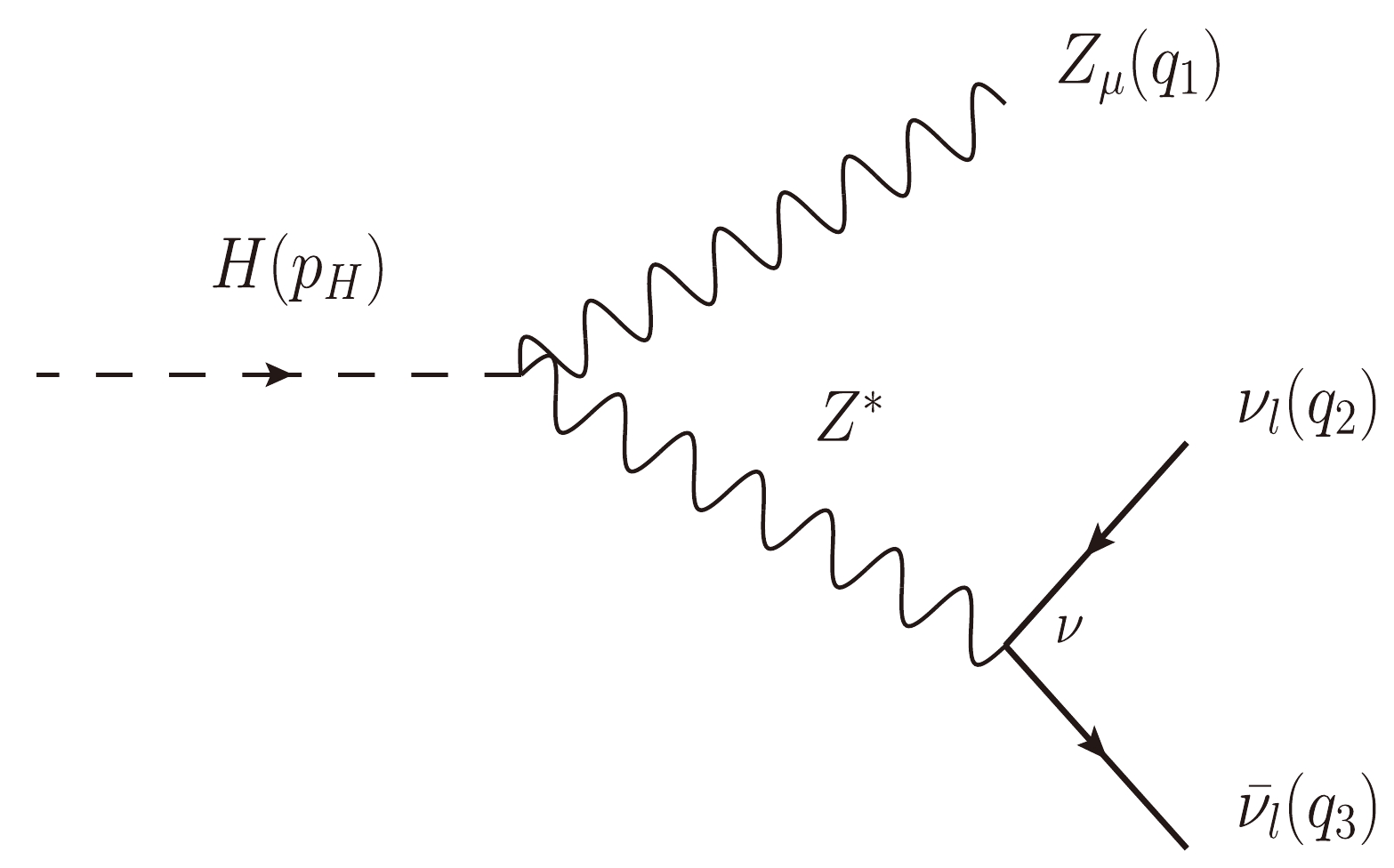
Figure E1. Group
$ G_0 $ : Tree level Feynman diagram.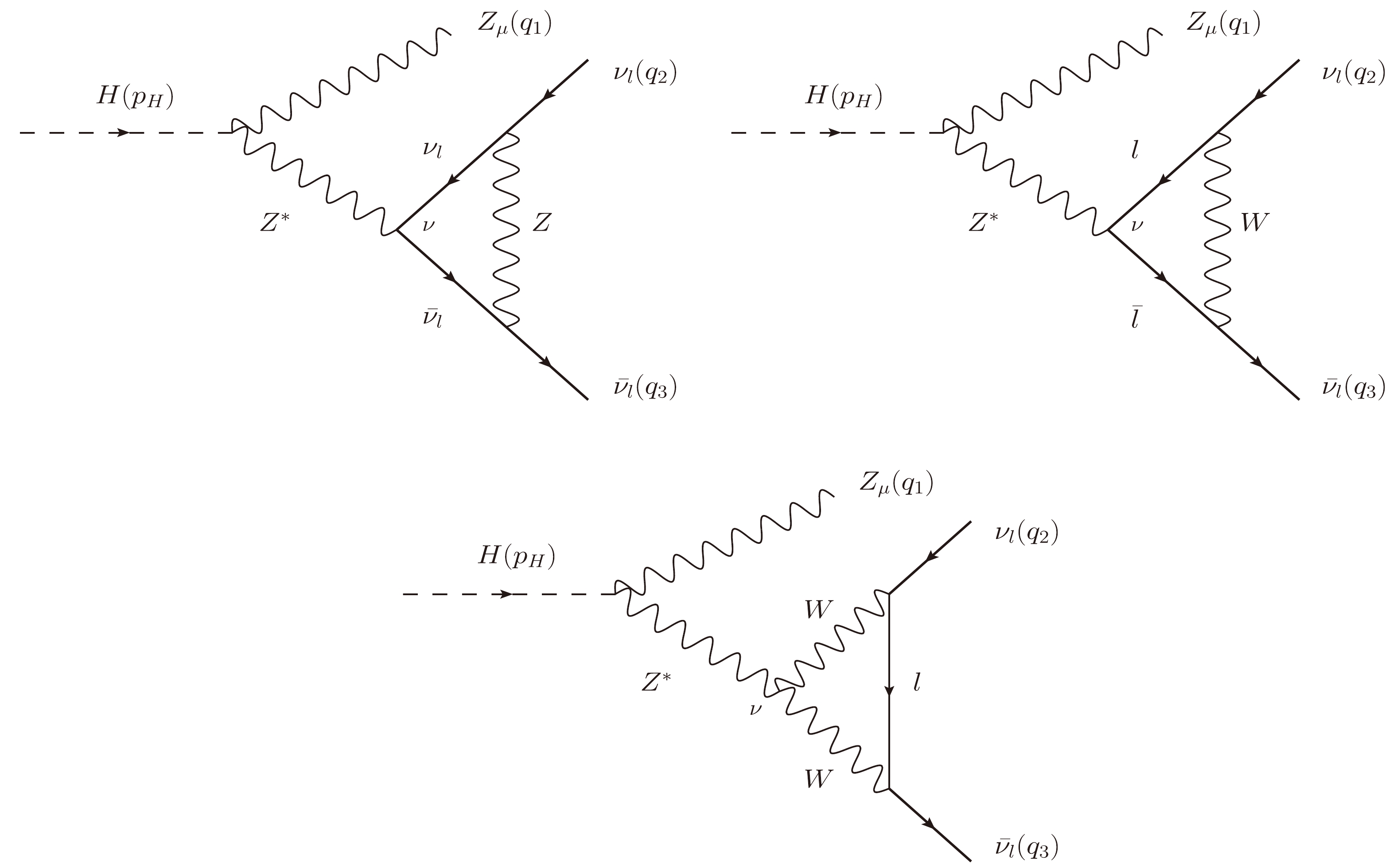
Figure E2. Group
$ G_1 $ : All one-loop Feynman diagrams contributing to the vertex$ H\nu_l\bar{\nu}_l $ .
Figure E3. Group
$ G_2 $ : All Z-pole Feynman diagrams contributing to the decay process. We note that$ \chi^{\pm} $ and$ c^{\pm} $ are Nambu-Goldstone bosons and ghost particles, respectively.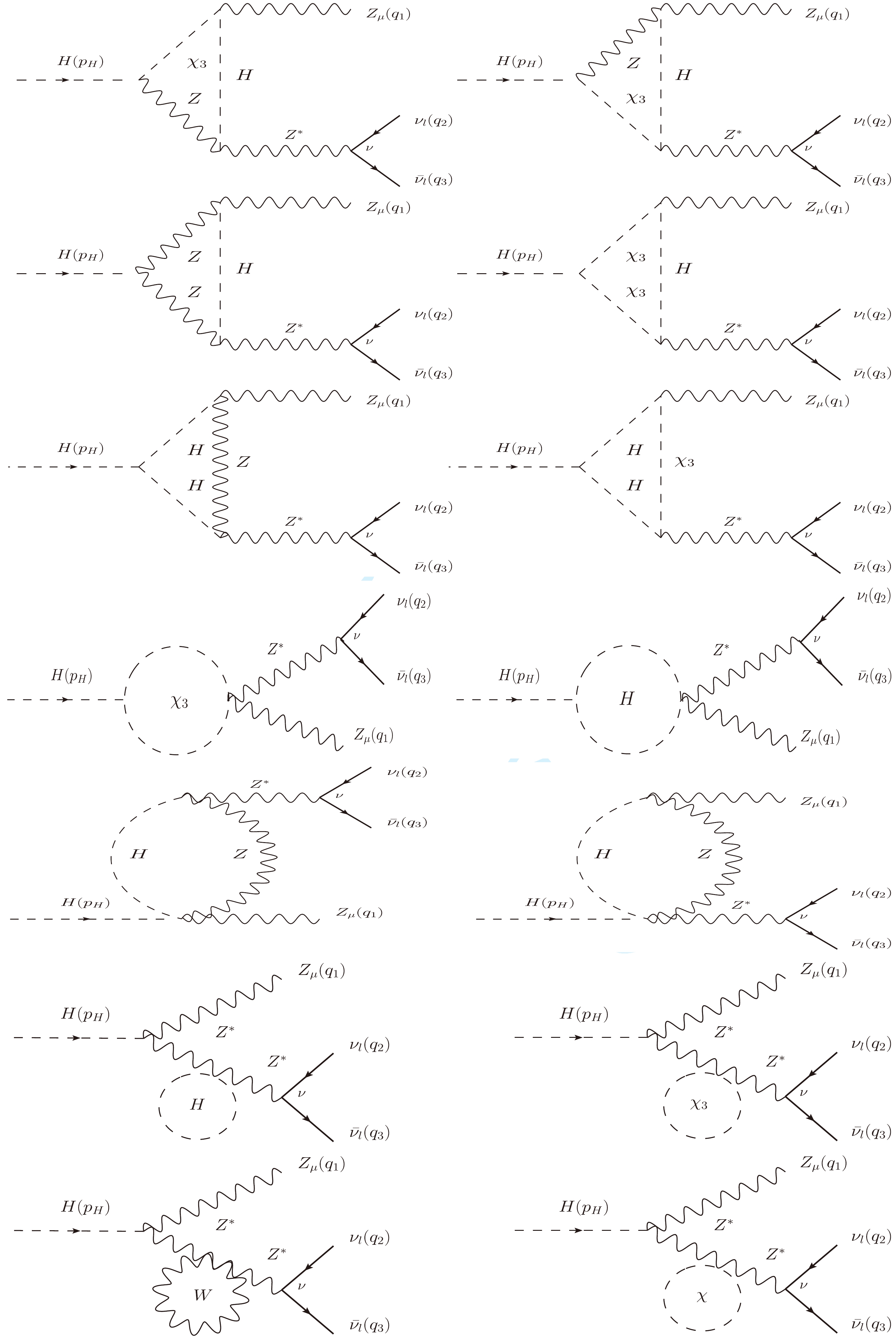
Figure E4. Group
$ G_2 $ : All Z-pole Feynman diagrams contributing to the decay process. We note that$ \chi_3 $ is Nambu-Goldstone boson.
Figure E5. Group
$ G_2 $ : All Z-pole Feynman diagrams contributing to the decay process. We note that$ \chi^{\pm} $ and$ c^{\pm} $ are Nambu-Goldstone bosons and ghost particles, respectively.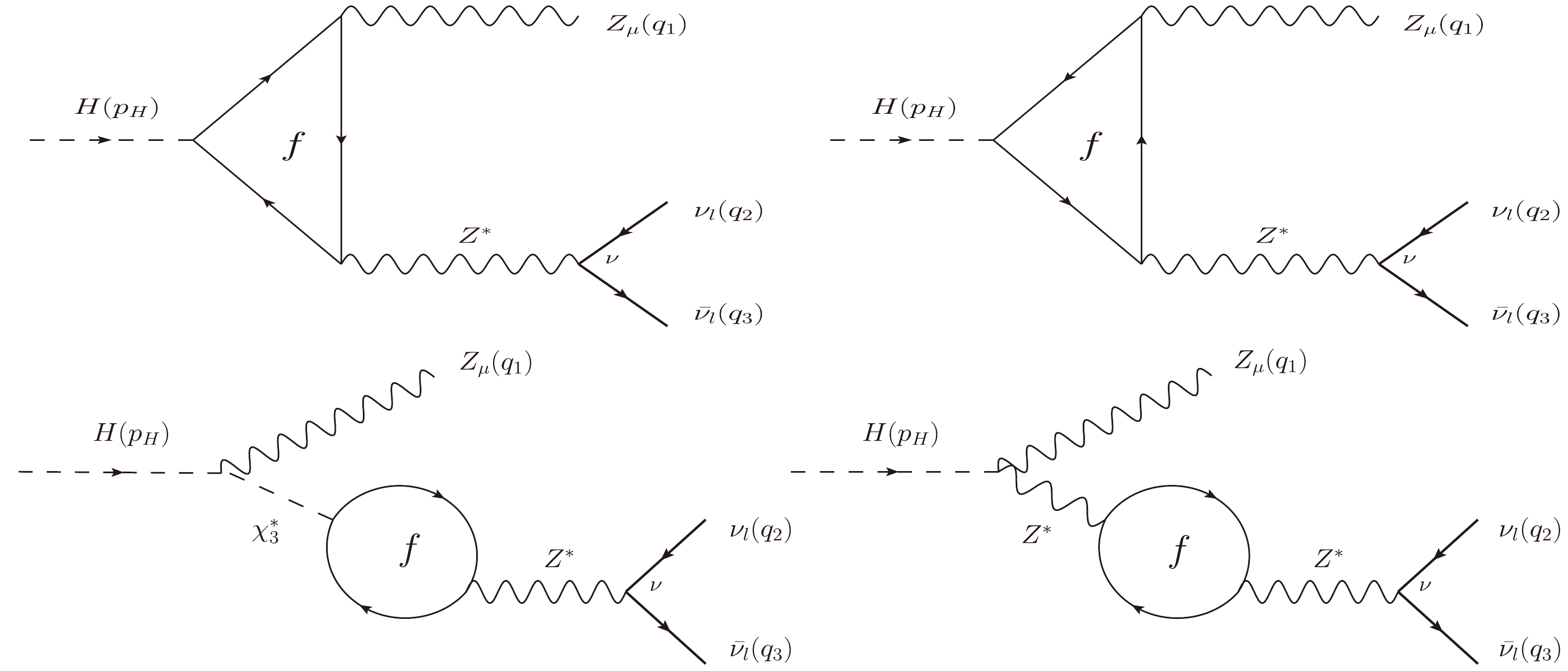
Figure E6. Group
$ G_2 $ : All Z-pole Feynman diagrams contributing to the decay process. Here,$ \chi_3 $ is Nambu-Goldstone boson.
Figure E7. Group
$ G_3 $ : All non Z-pole Feynman diagrams contributing to the decay process. Here$ \chi^{\pm} $ are Nambu-Goldstone bosons.

Figure E8. Group
$ G_4 $ : All counterterm Feynman diagrams contributing to the decay process.
One-loop formulas for H → Zνlνl for l = e, µ, τ in 't Hooft-Veltman gauge
- Received Date: 2023-01-16
- Available Online: 2023-05-15
Abstract: In this paper, we present analytical results for one-loop contributions to the decay processes


 DownLoad: