


 Abstract
 HTML
HTML Reference
 Related
 PDF
PDF


-
The quark model describes mesons as being composed of a quark and an antiquark (
$ q\bar{q} $ ), while quantum chromodynamics (QCD) allows the existence of exotic states. Exploring spin-exotic states is an important area of research. These states have exotic quantum numbers beyond those in the quark model, such as$ J^{PC} = 0^{--} $ , even+−, and odd−+, which can be easily identified.A hybrid state is an exotic state composed of a quark, an antiquark, and an excited gluon field, which reflects the gluonic degrees of freedom. The
$ 1^{-+} $ hybrid state, predicted by lattice QCD (LQCD) as the lightest hadron with spin-exotic quantum numbers, is estimated to have a mass in the range of 1.7−2.1 GeV/c2 [1]. Recently, LQCD investigated the production of$ 1^{-+} $ hybrid in$ J/\psi $ radiative decay and its possible decay modes [2, 3]. The isovector state$ \pi_1(1600) $ has long been considered an experimental candidate for the$ 1^{-+} $ spin-exotic nonet [4−7]. CLEO-c found a clear P-wave signal in the$ \eta^{\prime}\pi^{\pm} $ system around 1.6 GeV/$ c^2 $ from the$ \chi_{c1}\to\eta^{\prime}\pi^+\pi^- $ process [8]. Recently, the$ 1^{-+} $ isoscalar state$ \eta_1(1855) $ was discovered in the$ \eta\eta^{\prime} $ system by BESIII via$ J/\psi\to\gamma\eta\eta^{\prime} $ [9, 10], and it was considered a partner of$ \pi_1(1600) $ , marking a new research direction for spin-exotic states. These research results help understand the production mechanism of the$ 1^{-+} $ spin-exotic state.$ \eta_1(1855) $ can be observed via$ \chi_{c1}\to \eta_1(1855)\eta $ with$ \eta_1(1855)\to\eta\eta^{\prime} $ .Based on a sample of
$ 2.7\times10^{9} $ $ \psi(3686) $ events collected by the BESIII detector [11], the decay$ \psi(3686)\to \gamma\chi_{cJ} $ ,$ \chi_{cJ}\to\eta\eta\eta^{\prime} $ is analyzed in this study to search for$ \eta_{1}(1855) $ .$ \eta^{\prime} $ is reconstructed via$ \eta^{\prime}\to\gamma\pi^+\pi^- $ and$ \eta^{\prime}\to \eta\pi^+\pi^- $ , and η is reconstructed via$ \gamma\gamma $ . -
The BESIII detector [11] records symmetric
$ e^+e^- $ collisions provided by the BEPCII storage ring [12], with a center-of-mass energy ranging from 1.84 to 4.95 GeV and a peak luminosity of$ 1.1\times10^{33} $ cm−2s−1 achieved at$ \sqrt{s} = 3.773 $ GeV. BESIII has collected large data samples in this energy region [13]. The cylindrical core of the BESIII detector covers 93% of the full solid angle and includes a helium-based multilayer drift chamber (MDC), time-of-flight system (TOF), and CsI (Tl) electromagnetic calorimeter (EMC), which are all enclosed in a superconducting solenoidal magnet providing a 1.0 T magnetic field. The solenoid is supported by an octagonal flux-return yoke with resistive plate counter muon identification modules interleaved with steel. The charged-particle momentum resolution at$ 1\; {\rm{GeV}}/c $ is 0.5%, and the resolution of the specific ionization energy (dE/dx) is 6% for electrons from Bhabha scattering. The EMC measures photon energies with a resolution of 2.5% (5%) at 1 GeV in the barrel (end-cap) region. The time resolution in the TOF plastic scintillator barrel region is 68 ps, while that in the end-cap region is 110 ps. The end-cap TOF system was upgraded in 2015 using multi-gap resistive plate chamber technology, providing a time resolution of 60 ps. This benefitted 85% of the data used in this analysis [14−16].Monte Carlo (MC) simulated samples produced with GEANT4-based [17] software, which includes the geometric description of the BESIII detector and the detector response, are used to determine detection efficiencies and estimate backgrounds. The simulation models the beam energy spread and initial state radiation (ISR) in the
$ e^+e^- $ annihilations with the generator KKMC [18, 19]. The inclusive MC sample includes the production of the$ \psi(3686) $ resonance, ISR production of$ J/\psi $ , and continuum processes incorporated in KKMC [18, 19]. Known decay modes are modeled with EVTGEN [20, 21] using branching fractions taken from the Particle Data Group (PDG) [22]. The remaining unknown charmonium decays are modeled with LUNDCHARM [23, 24]. Final state radiation (FSR) from charged final state particles is incorporated using the PHOTOS package [25]. Exclusive MC samples are generated to determine the detection efficiency and optimize selection criteria. The signal is simulated with the E1 transition$ \psi(3686)\to\gamma\chi_{cJ} $ , where the polar angle θ of the radiative photon in the$ e^+e^- $ center-of-mass frame is distributed according to$(1+\lambda \cos^{2}\theta)$ . For$ J = 0 $ , 1, and 2, λ is set to be 1,$-{1}/{3}$ , and${1}/{13}$ , respectively [20, 21]. The decay$ \eta^{\prime}\to\gamma\pi^{+}\pi^{-} $ is simulated by a model that considers both the$ \rho-\omega $ interference and box anomaly [26], while the decay$ \eta^{\prime}\to\eta\pi^{+}\pi^{-} $ is simulated with a model based on the measured matrix elements [27]. Other processes are generated uniformly in phase space (PHSP). -
Charged tracks detected in the MDC are required to have a polar angle (θ) within the range of
$ |\cos\theta|<0.93 $ , where θ is defined with respect to the z-axis, which is the symmetry axis of the MDC. The distance of the closest approach to the interaction point (IP) must be less than 10 cm along the z-axis and less than 1 cm in the transverse plane. Two good charged tracks are required in the final state, and the total charge must be equal to zero.Particle identification (PID) for charged tracks combines measurements of the dE/dx in the MDC and the flight time in the TOF to form likelihoods
$ {\cal{L}}(h) $ $ (h = p, K, \pi) $ for each hadron (h) hypothesis. A charged track is identified as a pion when the pion hypothesis yields the maximum likelihood value, i.e.,$ {\cal{L}}(\pi)>{\cal{L}}(K) $ , and$ {\cal{L}}(\pi)>{\cal{L}}(p) $ . The two good charged tracks must both be identified as pions.For selecting good photon candidates, the deposited energy for the cluster must be larger than 25 MeV in the barrel (
$ |\cos \theta| < 0.80 $ ) or 50 MeV in the end-cap ($ 0.86 < |\cos \theta| < 0.92 $ ) regions. To exclude spurious photons caused by hadronic interactions and final state radiation, photon candidates must be at least$ 10^{\circ} $ away from any charged tracks when extrapolated to the EMC. The difference between the EMC time and event start time must be within [0, 700] ns for suppressing electronic noise and unrelated showers.For the
$ \psi(3686)\to\gamma\chi_{cJ} $ ,$ \chi_{cJ}\to\eta\eta\eta^{\prime} $ , and$ \eta^{\prime}\to\gamma\pi^+\pi^- $ modes, events are reconstructed with two oppositely charged tracks and at least six candidate photons. A six-constraint (6C) kinematic fit under the hypothesis of$ \psi(3686)\to\gamma\gamma\eta\eta\pi^+\pi^- $ is performed by imposing the energy-momentum conservation and constraining the mass of each pair of photons to the nominal η mass from the PDG [22]. If there is more than one combination, the one with the minimum$ \chi^2 $ value of the fit (denoted as$ \chi^2_{6{\rm{C}}} $ ) is retained. The result$ \chi^2_{6{\rm{C}}} $ needs to be less than 20, which is obtained by optimizing the figure of merit (FOM). The FOM is defined as$\text{FOM} = \dfrac{S}{\sqrt{S+B}}$ , where S represents the normalized number of signal events in the signal MC samples, and$ (S+B) $ corresponds to the number of data events. 4C kinematic fits are performed by imposing the energy-momentum conservation under the hypotheses of$ \psi(3686)\to 5\gamma\pi^{+}\pi^{-} $ ,$ \psi(3686)\to 6\gamma\pi^{+}\pi^{-} $ , and$ \psi(3686)\to 7\gamma\pi^{+}\pi^{-} $ to suppress backgrounds with five or seven photons in the final state.$ \chi^{2}_{\rm{4C}}(6\gamma\pi^{+}\pi^{-}) $ needs to be less than all possible$ \chi^{2}_{\rm{4C}}(5\gamma\pi^{+}\pi^{-}) $ and$ \chi^{2}_{\rm{4C}}(7\gamma\pi^{+}\pi^{-}) $ . To reconstruct the$ \eta^{\prime} $ candidate, the$ \gamma\pi^+\pi^- $ combination with the minimum$ |M(\gamma\pi^{+}\pi^{-})-m_{\eta^{\prime}}| $ is selected, where$ m_{\eta^{\prime}} $ represents the nominal$ \eta^{\prime} $ mass taken from the PDG [22]. Events with$ |M(\gamma\pi^{+}\pi^{-})-m_{\eta^{\prime}}|<0.01 $ GeV/$ c^{2} $ are selected for further analysis. To suppress backgrounds containing$ \pi^0 $ , events with$ |M(\gamma\gamma)-m_{\pi^{0}}|<0.02 $ GeV/$ c^{2} $ are rejected, where$ M(\gamma\gamma) $ represents the invariant mass of each photon pair except the two-photon pairs assigned to η, and$ m_{\pi^{0}} $ represents the nominal$ \pi^{0} $ mass [22]. The invariant mass distribution of$ \gamma\pi^+\pi^- $ is shown in Fig. 1(a).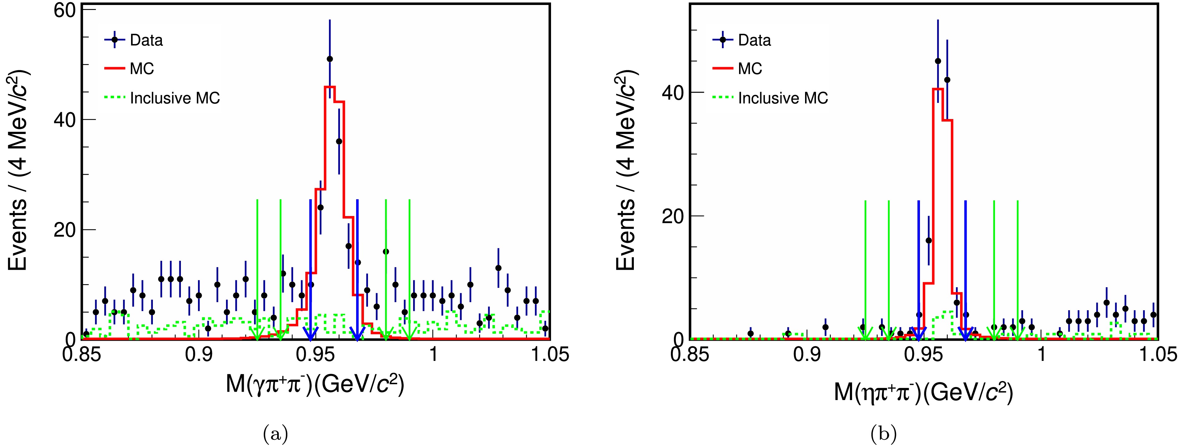
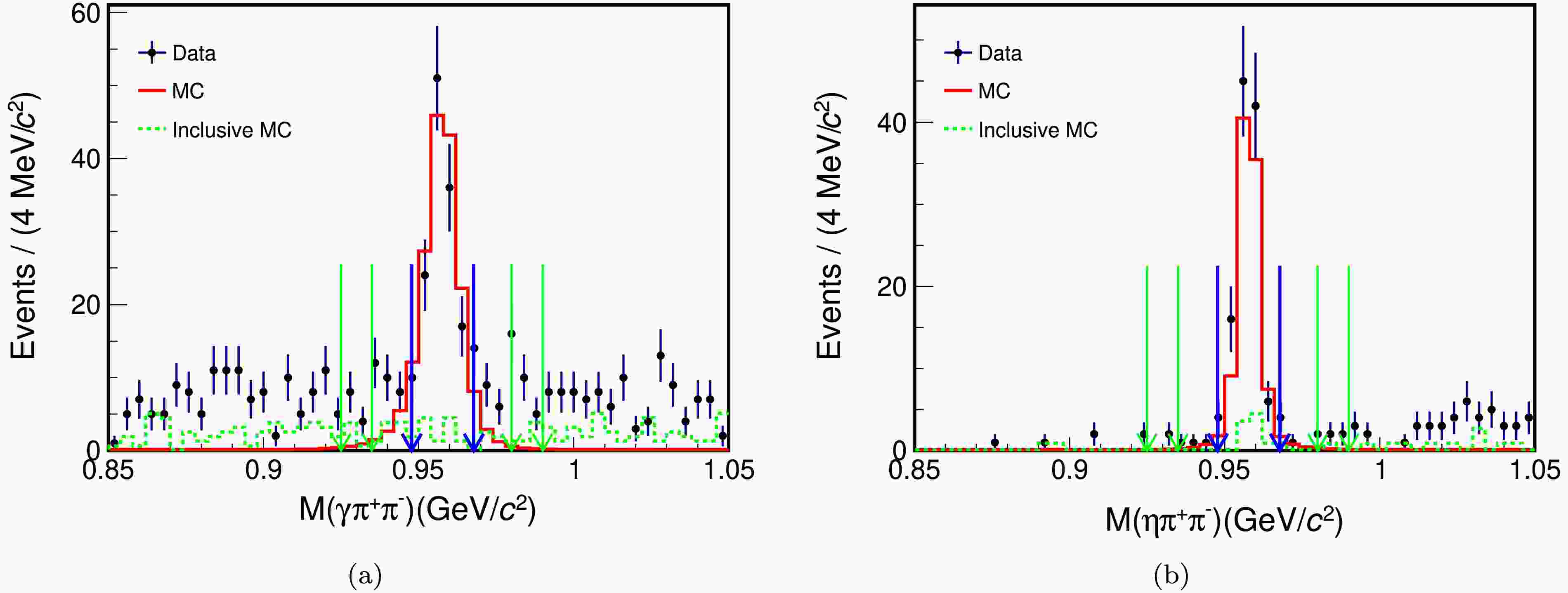
Figure 1. (color online) Invariant mass distributions of (a)
$ \eta^{\prime}\to\gamma\pi^+\pi^- $ and (b)$ \eta^{\prime}\to\eta\pi^+\pi^- $ within the entire$ \chi_{cJ} $ range (3.34−3.64 GeV/$ c^{2} $ ). The black points with error bars are data, the red solid histograms are the signal MC, and the green dashed histograms are the inclusive MC. The events between the blue arrows are the selected signal events, and the events between the green arrows on the same side are the selected sideband events.For the decays
$ \psi(3686)\to\gamma\chi_{cJ} $ ,$ \chi_{cJ}\to\eta\eta\eta^{\prime} $ ,$ \eta^{\prime}\to \eta\pi^+\pi^- $ , events are reconstructed with two oppositely charged tracks and at least seven candidate photons. A seven-constraint (7C) kinematic fit under the hypothesis of$ \psi(3686)\to\gamma\eta\eta\eta\pi^+\pi^- $ is performed by imposing the energy-momentum conservation and constraining the mass of each pair of photons to$ m_{\eta} $ . If there is more than one combination, the one with the minimum$ \chi^2 $ value of the fit (denoted as$ \chi^2_{7{\rm{C}}} $ ) is retained. The result$ \chi^2_{7{\rm{C}}} $ is required to be less than 55, which is obtained by optimizing the FOM,similarly to the optimization performed for the$ \eta^{\prime}\to\gamma\pi^+\pi^- $ mode. To suppress backgrounds with eight photons in the final state, 4C kinematic fits are performed by imposing the energy-momentum conservation under the hypotheses of$ \psi(3686)\to 6\gamma\pi^{+}\pi^{-} $ ,$ \psi(3686)\to 7\gamma\pi^{+}\pi^{-} $ , and$ \psi(3686)\to 8\gamma\pi^{+}\pi^{-} $ .$ \chi^{2}_{\rm{4C}}(7\gamma\pi^{+}\pi^{-}) $ needs to be less than$ \chi^{2}_{\rm{4C}}(8\gamma\pi^{+}\pi^{-}) $ . All selected events satisfy$ \chi^{2}_{\rm{4C}}(7\gamma\pi^{+}\pi^{-})<\chi^{2}_{\rm{4C}}(6\gamma\pi^{+}\pi^{-}) $ . The$ \eta\pi^+\pi^- $ combination with the minimum$ |M(\eta\pi^{+}\pi^{-})-m_{\eta^{\prime}}| $ is used to reconstruct the$ \eta^{\prime} $ candidate. Events with$ |M(\eta\pi^{+}\pi^{-})-m_{\eta^{\prime}}|<0.01 $ GeV/$ c^{2} $ are selected for further analysis. Backgrounds containing$ \pi^0 $ are suppressed by rejecting events with$ |M(\gamma\gamma)-m_{\pi^{0}}|< 0.02 $ GeV/$ c^{2} $ . The invariant mass distribution of$ \eta\pi^+\pi^- $ is shown in Fig. 1(b). -
Charged tracks detected in the MDC are required to have a polar angle (θ) within the range of
$ |\cos\theta|<0.93 $ , where θ is defined with respect to the z-axis, which is the symmetry axis of the MDC. The distance of the closest approach to the interaction point (IP) must be less than 10 cm along the z-axis and less than 1 cm in the transverse plane. Two good charged tracks are required in the final state, and the total charge must be equal to zero.Particle identification (PID) for charged tracks combines measurements of the dE/dx in the MDC and the flight time in the TOF to form likelihoods
$ {\cal{L}}(h) $ $ (h = p, K, \pi) $ for each hadron (h) hypothesis. A charged track is identified as a pion when the pion hypothesis yields the maximum likelihood value, i.e.,$ {\cal{L}}(\pi)>{\cal{L}}(K) $ , and$ {\cal{L}}(\pi)>{\cal{L}}(p) $ . The two good charged tracks must both be identified as pions.For selecting good photon candidates, the deposited energy for the cluster must be larger than 25 MeV in the barrel (
$ |\cos \theta| < 0.80 $ ) or 50 MeV in the end-cap ($ 0.86 < |\cos \theta| < 0.92 $ ) regions. To exclude spurious photons caused by hadronic interactions and final state radiation, photon candidates must be at least$ 10^{\circ} $ away from any charged tracks when extrapolated to the EMC. The difference between the EMC time and event start time must be within [0, 700] ns for suppressing electronic noise and unrelated showers.For the
$ \psi(3686)\to\gamma\chi_{cJ} $ ,$ \chi_{cJ}\to\eta\eta\eta^{\prime} $ , and$ \eta^{\prime}\to\gamma\pi^+\pi^- $ modes, events are reconstructed with two oppositely charged tracks and at least six candidate photons. A six-constraint (6C) kinematic fit under the hypothesis of$ \psi(3686)\to\gamma\gamma\eta\eta\pi^+\pi^- $ is performed by imposing the energy-momentum conservation and constraining the mass of each pair of photons to the nominal η mass from the PDG [22]. If there is more than one combination, the one with the minimum$ \chi^2 $ value of the fit (denoted as$ \chi^2_{6{\rm{C}}} $ ) is retained. The result$ \chi^2_{6{\rm{C}}} $ needs to be less than 20, which is obtained by optimizing the figure of merit (FOM). The FOM is defined as$\text{FOM} = \dfrac{S}{\sqrt{S+B}}$ , where S represents the normalized number of signal events in the signal MC samples, and$ (S+B) $ corresponds to the number of data events. 4C kinematic fits are performed by imposing the energy-momentum conservation under the hypotheses of$ \psi(3686)\to 5\gamma\pi^{+}\pi^{-} $ ,$ \psi(3686)\to 6\gamma\pi^{+}\pi^{-} $ , and$ \psi(3686)\to 7\gamma\pi^{+}\pi^{-} $ to suppress backgrounds with five or seven photons in the final state.$ \chi^{2}_{\rm{4C}}(6\gamma\pi^{+}\pi^{-}) $ needs to be less than all possible$ \chi^{2}_{\rm{4C}}(5\gamma\pi^{+}\pi^{-}) $ and$ \chi^{2}_{\rm{4C}}(7\gamma\pi^{+}\pi^{-}) $ . To reconstruct the$ \eta^{\prime} $ candidate, the$ \gamma\pi^+\pi^- $ combination with the minimum$ |M(\gamma\pi^{+}\pi^{-})-m_{\eta^{\prime}}| $ is selected, where$ m_{\eta^{\prime}} $ represents the nominal$ \eta^{\prime} $ mass taken from the PDG [22]. Events with$ |M(\gamma\pi^{+}\pi^{-})-m_{\eta^{\prime}}|<0.01 $ GeV/$ c^{2} $ are selected for further analysis. To suppress backgrounds containing$ \pi^0 $ , events with$ |M(\gamma\gamma)-m_{\pi^{0}}|<0.02 $ GeV/$ c^{2} $ are rejected, where$ M(\gamma\gamma) $ represents the invariant mass of each photon pair except the two-photon pairs assigned to η, and$ m_{\pi^{0}} $ represents the nominal$ \pi^{0} $ mass [22]. The invariant mass distribution of$ \gamma\pi^+\pi^- $ is shown in Fig. 1(a).
Figure 1. (color online) Invariant mass distributions of (a)
$ \eta^{\prime}\to\gamma\pi^+\pi^- $ and (b)$ \eta^{\prime}\to\eta\pi^+\pi^- $ within the entire$ \chi_{cJ} $ range (3.34−3.64 GeV/$ c^{2} $ ). The black points with error bars are data, the red solid histograms are the signal MC, and the green dashed histograms are the inclusive MC. The events between the blue arrows are the selected signal events, and the events between the green arrows on the same side are the selected sideband events.For the decays
$ \psi(3686)\to\gamma\chi_{cJ} $ ,$ \chi_{cJ}\to\eta\eta\eta^{\prime} $ ,$ \eta^{\prime}\to \eta\pi^+\pi^- $ , events are reconstructed with two oppositely charged tracks and at least seven candidate photons. A seven-constraint (7C) kinematic fit under the hypothesis of$ \psi(3686)\to\gamma\eta\eta\eta\pi^+\pi^- $ is performed by imposing the energy-momentum conservation and constraining the mass of each pair of photons to$ m_{\eta} $ . If there is more than one combination, the one with the minimum$ \chi^2 $ value of the fit (denoted as$ \chi^2_{7{\rm{C}}} $ ) is retained. The result$ \chi^2_{7{\rm{C}}} $ is required to be less than 55, which is obtained by optimizing the FOM,similarly to the optimization performed for the$ \eta^{\prime}\to\gamma\pi^+\pi^- $ mode. To suppress backgrounds with eight photons in the final state, 4C kinematic fits are performed by imposing the energy-momentum conservation under the hypotheses of$ \psi(3686)\to 6\gamma\pi^{+}\pi^{-} $ ,$ \psi(3686)\to 7\gamma\pi^{+}\pi^{-} $ , and$ \psi(3686)\to 8\gamma\pi^{+}\pi^{-} $ .$ \chi^{2}_{\rm{4C}}(7\gamma\pi^{+}\pi^{-}) $ needs to be less than$ \chi^{2}_{\rm{4C}}(8\gamma\pi^{+}\pi^{-}) $ . All selected events satisfy$ \chi^{2}_{\rm{4C}}(7\gamma\pi^{+}\pi^{-})<\chi^{2}_{\rm{4C}}(6\gamma\pi^{+}\pi^{-}) $ . The$ \eta\pi^+\pi^- $ combination with the minimum$ |M(\eta\pi^{+}\pi^{-})-m_{\eta^{\prime}}| $ is used to reconstruct the$ \eta^{\prime} $ candidate. Events with$ |M(\eta\pi^{+}\pi^{-})-m_{\eta^{\prime}}|<0.01 $ GeV/$ c^{2} $ are selected for further analysis. Backgrounds containing$ \pi^0 $ are suppressed by rejecting events with$ |M(\gamma\gamma)-m_{\pi^{0}}|< 0.02 $ GeV/$ c^{2} $ . The invariant mass distribution of$ \eta\pi^+\pi^- $ is shown in Fig. 1(b). -
Potential backgrounds are studied using the inclusive MC samples of
$ \psi(3686) $ decays. The backgrounds fall into three categories: non-$ \chi_{cJ} $ , non-$ \eta^{\prime} $ , and processes involving both$ \eta^{\prime} $ and$ \chi_{cJ} $ . Non-$ \chi_{cJ} $ backgrounds are modeled using a polynomial function when fitting the invariant mass distributions of$ \eta\eta\eta^{\prime} $ . Non-$ \eta^{\prime} $ backgrounds are estimated using the$ \eta^{\prime} $ mass sidebands in the data. The sideband regions for$ \eta^{\prime} $ are defined as [0.925, 0.935] and [0.98, 0.99] GeV/$ c^{2} $ . The$ \eta^{\prime} $ signal shape is determined from the shape of the signal MC sample, and the$ \eta^{\prime} $ sideband shape is described by a linear function. Backgrounds containing both$ \chi_{cJ} $ and$ \eta^{\prime} $ are peaking backgrounds. To estimate the peaking backgrounds, exclusive MC samples with high statistics are generated for these peaking background processes as indicated in the inclusive MC. The peaking background contributions are normalized with the corresponding branching fractions from PDG and efficiency obtained from the background MC samples, which are then fixed in the fit. The peaking backgrounds for the decay mode$ \eta^{\prime}\to\gamma\pi^+\pi^- $ arise from$ \chi_{c1}\to\gamma J/\psi,\, J/\psi\to\gamma\eta\eta^{\prime} $ and$ \chi_{c2}\to\gamma J/\psi, J/\psi\to\gamma\eta\eta^{\prime} $ , with estimated yields (fractions) of 2.35 (1.7%) and 1.14 (0.8%), respectively. Similarly, the peaking backgrounds for the decay mode$ \eta^{\prime}\to\eta\pi^+\pi^- $ arise from$ \chi_{c1}\to \gamma J/\psi, J/\psi\to \gamma\eta\eta' $ ,$ \chi_{c2}\to\gamma J/\psi, J/\psi\to\gamma\eta\eta' $ and$ \chi_{c0}\to \eta^{\prime}\eta^{\prime} $ , with estimated yields (fractions) of 1.97 (1.7%), 0.82 (0.7%) and 1.25 (1.1%), respectively. The backgrounds with a fraction of no more than 1.0% are neglected. -
The
$ \eta\eta\eta^{\prime} $ invariant mass distributions for the$ \eta^{\prime}\to \gamma\pi^{+}\pi^{-} $ and$ \eta^{\prime}\to\eta\pi^{+}\pi^{-} $ modes are shown in Fig. 2. We perform a simultaneous unbinned maximum likelihood fit to the$ \eta\eta\eta^{\prime} $ distributions in the range of [3.34, 3.64] GeV/$ c^{2} $ . The$ \chi_{c0} $ ,$ \chi_{c1} $ , and$ \chi_{c2} $ signals are modeled using the shape of MC samples convolved with a Gaussian function to consider the mass resolution and describe the difference between data and MC simulation. Parameters of the Gaussian function are shared among the$ \chi_{c0} $ ,$ \chi_{c1} $ , and$ \chi_{c2} $ signals and left free in the fit. The peaking backgrounds are normalized and fixed based on the MC simulations. The non-$ \eta^{\prime} $ background events are described by the$ \eta^{\prime} $ mass sidebands and fixed in the fit. The remaining background is described by a linear function with free parameters. In the simultaneous fit, the fitted yields of$ {\cal{N}}_{\text{sig}, 1} $ and$ {\cal{N}}_{\text{sig}, 2} $ are constrained to the common number of produced$ \chi_{cJ}\to\eta\eta\eta^{\prime} $ events$ {\cal{N}}^{\chi_{cJ}}_{\text{sig}} $ , which is defined as
Figure 2. (color online) Simultaneous fit results for the invariant mass distributions of
$ \eta\eta\eta^{\prime} $ in two decay modes of$ \eta^{\prime} $ (a)$ \eta^{\prime}\to\gamma\pi^+\pi^- $ and (b)$ \eta^{\prime}\to\eta\pi^+\pi^- $ . The dots with error bars represent the data; the red solid curves show the fit results; and the dark green, light green, and blue dashed lines represent the signals of$ \chi_{c0} $ ,$ \chi_{c1} $ , and$ \chi_{c2} $ , respectively, while the other dashed lines represent the backgrounds.$ \begin{aligned}[b] {\cal{N}}^{\chi_{cJ}}_{\text{sig}} =\;& \frac{{\cal{N}}_{\text{sig}, 1}}{\epsilon_{1} \cdot {\cal{B}}(\eta^{\prime}\to\gamma\pi^+\pi^-) \cdot {\cal{B}}(\eta\to\gamma\gamma)^2} \\ =\;& \frac{{\cal{N}}_{\text{sig}, 2}}{\epsilon_{2} \cdot {\cal{B}}(\eta^{\prime}\to\eta\pi^+\pi^-) \cdot {\cal{B}}(\eta\to\gamma\gamma)^3}, \end{aligned}$

(1) where indices 1 and 2 represent
$ \eta^{\prime}\to\gamma\pi^{+}\pi^{-} $ and$ \eta^{\prime}\to \eta\pi^{+}\pi^{-} $ , respectively.$ {\cal{N}}_{\text{sig}, 1} $ and$ {\cal{N}}_{\text{sig}, 2} $ are the numbers of observed$ \chi_{cJ} $ events,$ \epsilon_{1} $ and$ \epsilon_{2} $ represent the corresponding detection efficiencies, and the branching fractions are obtained from the PDG [22]. The fit result is shown in Fig. 2.The branching fractions of
$ \chi_{cJ}\to\eta\eta\eta^{\prime} $ are calculated by$ {\cal{B}}(\chi_{cJ}\to\eta\eta\eta^{\prime}) = \frac{ {\cal{N}}^{ \chi_{cJ}}_{\text{sig}} }{ N_{\psi(3686)} \cdot {\cal{B}}(\psi(3686)\to\gamma\chi_{cJ})}, $

(2) where
$ {\cal{N}}^{ \chi_{cJ}}_{\text{sig}} $ is defined in Eq. (1),$ N_{\psi(3686)} $ represents the number of$ \psi(3686) $ events, and$ {\cal{B}}(\psi(3686)\to\gamma\chi_{cJ}) $ represents the branching fraction of$ \psi(3686)\to\gamma\chi_{cJ} $ obtained from PDG [22]. As no clear signal for$ \chi_{c0} $ exists, a Bayesian method is used to obtain the upper limit of the signal yield at 90% confidence level (CL). To determine the upper limit of the signal yield, the distribution of normalized likelihood values for a series of expected signal yields is considered as the probability density function (PDF). For obtaining the distribution of likelihood values, the signals of$ \chi_{c1} $ and$ \chi_{c2} $ are described by the MC shape function convolved with a Gaussian function, and their parameters are free. The upper limit of the signal yields at a 90% CL, denoted as$ N^{\text{UL}} $ , is defined as the number of events where 90% of the PDF area lies above zero. These results of branching fractions are listed in Table 1. The statistical significances of$ \chi_{c0} $ ,$ \chi_{c1} $ , and$ \chi_{c2} $ are evaluated based on the change of the likelihood value when they are included, considering the change in the number of degrees of freedom.$ \chi_{cJ} $ 

$ {\cal{N}}_{\text{sig}, 1} $ 

$ \epsilon_1 $ (%)

$ {\cal{N}}_{\text{sig}, 2} $ 

$ \epsilon_2 $ (%)

$ {\cal{N}}^{ \chi_{cJ}}_{\text{sig}} $ 

$ {\cal{B}}(\chi_{cJ}\to\eta\eta\eta^{\prime}) $ 

Significance $ \chi_{c0} $ 

$ 9.1 \pm 3.9 $ 

$ 5.23\pm0.02 $ 

$ 3.8 \pm 1.6 $ 

$ 3.86\pm 0.02 $ 

$ 3809.6\pm 1607.6 $ 

- $ 1.4\sigma $ 

$ \chi_{c1} $ 

$ 97.7\pm 9.1 $ 

$ 5.76\pm 0.02 $ 

$ 38.8 \pm 3.6 $ 

$ 4.03\pm 0.02 $ 

$ 37016.9\pm 3431.3 $ 

$ (1.40 \pm 0.13 \pm 0.09)\times 10^{-4} $ 

$ 16.8\sigma $ 

$ \chi_{c2} $ 

$ 26.3\pm 5.3 $ 

$ 5.32\pm 0.02 $ 

$ 10.4 \pm 2.1 $ 

$ 3.70\pm 0.02 $ 

$ 10783.4\pm 2162.44 $ 

$ (4.18 \pm 0.84 \pm 0.48)\times 10^{-5} $ 

$ 7.2\sigma $ 

Table 1. Number of observed
$ \chi_{cJ} $ events ($ {\cal{N}}_{\text{sig},1} $ and$ {\cal{N}}_{\text{sig},2} $ ), corresponding detection efficiencies ($ \epsilon_1 $ and$ \epsilon_2 $ ), number of produced$ \chi_{cJ}\to\eta\eta\eta^{\prime} $ events ($ {\cal{N}}^{ \chi_{cJ}}_{\text{sig}} $ , which is defined in Eq. (1)), branching fractions ($ {\cal{B}} $ ), and statistical significance. Indices 1 and 2 represent$ \eta^{\prime}\to\gamma\pi^+\pi^- $ and$ \eta^{\prime}\to\eta\pi^+\pi^- $ , respectively. The first and second uncertainties are statistical and systematic, respectively. -
The
$ \eta\eta\eta^{\prime} $ invariant mass distributions for the$ \eta^{\prime}\to \gamma\pi^{+}\pi^{-} $ and$ \eta^{\prime}\to\eta\pi^{+}\pi^{-} $ modes are shown in Fig. 2. We perform a simultaneous unbinned maximum likelihood fit to the$ \eta\eta\eta^{\prime} $ distributions in the range of [3.34, 3.64] GeV/$ c^{2} $ . The$ \chi_{c0} $ ,$ \chi_{c1} $ , and$ \chi_{c2} $ signals are modeled using the shape of MC samples convolved with a Gaussian function to consider the mass resolution and describe the difference between data and MC simulation. Parameters of the Gaussian function are shared among the$ \chi_{c0} $ ,$ \chi_{c1} $ , and$ \chi_{c2} $ signals and left free in the fit. The peaking backgrounds are normalized and fixed based on the MC simulations. The non-$ \eta^{\prime} $ background events are described by the$ \eta^{\prime} $ mass sidebands and fixed in the fit. The remaining background is described by a linear function with free parameters. In the simultaneous fit, the fitted yields of$ {\cal{N}}_{\text{sig}, 1} $ and$ {\cal{N}}_{\text{sig}, 2} $ are constrained to the common number of produced$ \chi_{cJ}\to\eta\eta\eta^{\prime} $ events$ {\cal{N}}^{\chi_{cJ}}_{\text{sig}} $ , which is defined as
Figure 2. (color online) Simultaneous fit results for the invariant mass distributions of
$ \eta\eta\eta^{\prime} $ in two decay modes of$ \eta^{\prime} $ (a)$ \eta^{\prime}\to\gamma\pi^+\pi^- $ and (b)$ \eta^{\prime}\to\eta\pi^+\pi^- $ . The dots with error bars represent the data; the red solid curves show the fit results; and the dark green, light green, and blue dashed lines represent the signals of$ \chi_{c0} $ ,$ \chi_{c1} $ , and$ \chi_{c2} $ , respectively, while the other dashed lines represent the backgrounds.$ \begin{aligned}[b] {\cal{N}}^{\chi_{cJ}}_{\text{sig}} =\;& \frac{{\cal{N}}_{\text{sig}, 1}}{\epsilon_{1} \cdot {\cal{B}}(\eta^{\prime}\to\gamma\pi^+\pi^-) \cdot {\cal{B}}(\eta\to\gamma\gamma)^2} \\ =\;& \frac{{\cal{N}}_{\text{sig}, 2}}{\epsilon_{2} \cdot {\cal{B}}(\eta^{\prime}\to\eta\pi^+\pi^-) \cdot {\cal{B}}(\eta\to\gamma\gamma)^3}, \end{aligned}$
(1) where indices 1 and 2 represent
$ \eta^{\prime}\to\gamma\pi^{+}\pi^{-} $ and$ \eta^{\prime}\to \eta\pi^{+}\pi^{-} $ , respectively.$ {\cal{N}}_{\text{sig}, 1} $ and$ {\cal{N}}_{\text{sig}, 2} $ are the numbers of observed$ \chi_{cJ} $ events,$ \epsilon_{1} $ and$ \epsilon_{2} $ represent the corresponding detection efficiencies, and the branching fractions are obtained from the PDG [22]. The fit result is shown in Fig. 2.The branching fractions of
$ \chi_{cJ}\to\eta\eta\eta^{\prime} $ are calculated by$ {\cal{B}}(\chi_{cJ}\to\eta\eta\eta^{\prime}) = \frac{ {\cal{N}}^{ \chi_{cJ}}_{\text{sig}} }{ N_{\psi(3686)} \cdot {\cal{B}}(\psi(3686)\to\gamma\chi_{cJ})}, $
(2) where
$ {\cal{N}}^{ \chi_{cJ}}_{\text{sig}} $ is defined in Eq. (1),$ N_{\psi(3686)} $ represents the number of$ \psi(3686) $ events, and$ {\cal{B}}(\psi(3686)\to\gamma\chi_{cJ}) $ represents the branching fraction of$ \psi(3686)\to\gamma\chi_{cJ} $ obtained from PDG [22]. As no clear signal for$ \chi_{c0} $ exists, a Bayesian method is used to obtain the upper limit of the signal yield at 90% confidence level (CL). To determine the upper limit of the signal yield, the distribution of normalized likelihood values for a series of expected signal yields is considered as the probability density function (PDF). For obtaining the distribution of likelihood values, the signals of$ \chi_{c1} $ and$ \chi_{c2} $ are described by the MC shape function convolved with a Gaussian function, and their parameters are free. The upper limit of the signal yields at a 90% CL, denoted as$ N^{\text{UL}} $ , is defined as the number of events where 90% of the PDF area lies above zero. These results of branching fractions are listed in Table 1. The statistical significances of$ \chi_{c0} $ ,$ \chi_{c1} $ , and$ \chi_{c2} $ are evaluated based on the change of the likelihood value when they are included, considering the change in the number of degrees of freedom.$ \chi_{cJ} $ $ {\cal{N}}_{\text{sig}, 1} $ $ \epsilon_1 $ (%)$ {\cal{N}}_{\text{sig}, 2} $ $ \epsilon_2 $ (%)$ {\cal{N}}^{ \chi_{cJ}}_{\text{sig}} $ $ {\cal{B}}(\chi_{cJ}\to\eta\eta\eta^{\prime}) $ Significance $ \chi_{c0} $ $ 9.1 \pm 3.9 $ $ 5.23\pm0.02 $ $ 3.8 \pm 1.6 $ $ 3.86\pm 0.02 $ $ 3809.6\pm 1607.6 $ - $ 1.4\sigma $ $ \chi_{c1} $ $ 97.7\pm 9.1 $ $ 5.76\pm 0.02 $ $ 38.8 \pm 3.6 $ $ 4.03\pm 0.02 $ $ 37016.9\pm 3431.3 $ $ (1.40 \pm 0.13 \pm 0.09)\times 10^{-4} $ $ 16.8\sigma $ $ \chi_{c2} $ $ 26.3\pm 5.3 $ $ 5.32\pm 0.02 $ $ 10.4 \pm 2.1 $ $ 3.70\pm 0.02 $ $ 10783.4\pm 2162.44 $ $ (4.18 \pm 0.84 \pm 0.48)\times 10^{-5} $ $ 7.2\sigma $ Table 1. Number of observed
$ \chi_{cJ} $ events ($ {\cal{N}}_{\text{sig},1} $ and$ {\cal{N}}_{\text{sig},2} $ ), corresponding detection efficiencies ($ \epsilon_1 $ and$ \epsilon_2 $ ), number of produced$ \chi_{cJ}\to\eta\eta\eta^{\prime} $ events ($ {\cal{N}}^{ \chi_{cJ}}_{\text{sig}} $ , which is defined in Eq. (1)), branching fractions ($ {\cal{B}} $ ), and statistical significance. Indices 1 and 2 represent$ \eta^{\prime}\to\gamma\pi^+\pi^- $ and$ \eta^{\prime}\to\eta\pi^+\pi^- $ , respectively. The first and second uncertainties are statistical and systematic, respectively. -
The systematic uncertainties of
$ {\cal{B}}(\chi_{cJ}\to\eta\eta\eta^{\prime}) $ are summarized below.1. Number of
$ \psi(3686) $ events. The number of$ \psi(3686) $ events is determined by analyzing inclusive hadronic$ \psi(3686) $ decays with an uncertainty of 0.5% [28].2. MDC tracking. The data-MC efficiency difference for pion track-finding is studied using a control sample of
$ J/\psi\to\rho\pi $ and$ J/\psi\to p\bar{p}\pi^{+}\pi^{-} $ [29]. The systematic uncertainty from MDC tracking is 1.0% per charged pion.3. PID. The pion PID efficiency for data agrees within 1.0% with that of the MC simulation in the pion momentum region, as reported in [29]. Thus, a systematic uncertainty of 2.0% is assigned to PID.
4. Photon reconstruction. For photons detected by the EMC, the detection efficiency is studied using a control sample of
$ e^+e^-\to\gamma_{\text{ISR}}\mu^+\mu^- $ , where ISR stands for initial state radiation. The systematic uncertainty, defined as the relative difference in efficiencies between data and MC simulation, is observed to be up to 0.5% per photon in both the barrel and end-cap regions.5. Intermediate decay branching fractions. The uncertainties on the intermediate decay branching fractions are taken from the PDG values [22].
6. Kinematic fit. The track helix parameter correction method is used to investigate the systematic uncertainty associated with the kinematic fit [30]. The difference in the detection efficiencies with and without the helix correction is considered the systematic uncertainty.
7. Mass windows of
$ \eta^{\prime} $ and$ \chi_{cJ} $ . The systematic uncertainty from the requirement on the$ \eta^{\prime} $ or$ \chi_{cJ} $ signal region is estimated by smearing the$ \gamma\pi^{+}\pi^{-} $ ($ \eta\pi^{+}\pi^{-} $ ) and$ \eta\eta\eta^{\prime} $ invariant masses in the signal MC sample with a Gaussian function to account for the resolution difference between data and MC simulation. The smearing parameters are determined by fitting the$ \gamma\pi^{+}\pi^{-} $ ($ \eta\pi^{+}\pi^{-} $ ) and$ \eta\eta\eta^{\prime} $ invariant mass distributions in data with the MC shape convolved with a Gaussian function. The difference in the detection efficiency, as determined from the signal MC sample with and without the extra smearing, is used as the systematic uncertainty.8. Veto of
$ \pi^0 $ . Possible systematic effects caused by the veto on$ \pi^0 $ are investigated using the Barlow test [31] by varying the veto criteria between 10 and 50 MeV/$ c^2 $ . The uncertainty is assigned as the difference between the nominal result and result with$ |M(\gamma\gamma)-m_{\pi^0}|<21 $ MeV/$ c^2 $ when 95% of the candidate events are retained. There is no signal in the$ \chi_{c0} $ process, and therefore, we set the value of this systematic uncertainty to be the same as that for$ \chi_{c1,\, c2} $ .9. Fit range. Systematic uncertainties caused by different fit ranges are examined by enlarging and shrinking the fit range eight times, with a step of 20 MeV/
$ c^2 $ . For each case, the deviation between the alternative and nominal fits is defined as$\xi = \dfrac{|a_1-a_2|}{\sqrt{|\sigma_1^2-\sigma_2^2|}}$ , where$ a_1\pm \sigma_1 $ and$ a_2\pm\sigma_2 $ are the nominal and alternative fit results, respectively. If ξ is less than 2.0, the associated systematic uncertainty is negligible according to the Barlow test [31]. The largest difference is assigned as the systematic uncertainty.10. Non-peaking background shape. The systematic uncertainty caused by the background shape is estimated by replacing the linear function with a second-order polynomial in the fit. The maximum difference in the signal yields compared to the nominal value is considered as the uncertainty.
11.
$ \eta^{\prime} $ sideband. The uncertainties from the$ \eta^{\prime} $ sideband region are estimated by changing sideband regions to [0.93, 0.94] and [0.975, 0.985] GeV/$ c^{2} $ . The maximum difference in the signal yields compared to the nominal value is considered as the uncertainty.12. Peaking background. The uncertainties from the peaking background are estimated by changing the fixed number of peaking background events, which is calculated through the propagation of branching fraction errors. The fixed branching fraction values of the peaking background are calculated by adding or subtracting
$ 1\sigma $ from the nominal value of these processes. The maximum difference in signal yields compared to the nominal value is considered as the uncertainty.For the two
$ \eta^{\prime} $ decay modes, some systematic uncertainties are common, while others are independent. The combination of common and independent systematic uncertainties for these two decay modes are calculated using the weighted least squares method [32].The sources of systematic uncertainties used for calculating
$ {\cal{B}}(\chi_{c1,\, c2} \to\eta\eta\eta^{\prime}) $ are listed in Table 2. Their branching fractions are determined to be$ {\cal{B}}(\chi_{c1}\to\eta\eta\eta^{\prime}) = (1.40\, \pm 0.13\, (\text{stat.}) \pm 0.09\, (\text{sys.}))\times 10^{-4} $ and$ {\cal{B}}(\chi_{c2}\to\eta\eta\eta^{\prime}) = (4.18\, \pm 0.84\, (\text{stat.}) \pm 0.48\, (\text{sys.}))\times 10^{-5} $ . Further,$ {\cal{B}}(\chi_{c1}\to \pi^+\pi^-\eta^{\prime}) = (2.2\pm 0.4)\times 10^{-3} $ and$ {\cal{B}}(\chi_{c2}\to \pi^+\pi^-\eta^{\prime}) = (5.1\pm 1.9)\times 10^{-4} $ [22]. In comparison, the branching fractions of$ \chi_{c1,\, c2}\to\eta\eta\eta^{\prime} $ obtained in this analysis are an order of magnitude smaller than those of$ \chi_{c1,\, c2}\to\pi^+\pi^-\eta^{\prime} $ .Independent systematic uncertainties Source $ \chi_{c1} $ 

$ \chi_{c2} $ 

$ \gamma\pi^{+}\pi^{-} $ 

$ \eta\pi^{+}\pi^{-} $ 

$ \gamma\pi^{+}\pi^{-} $ 

$ \eta\pi^{+}\pi^{-} $ 

Another photon reconstruction − 0.5 − 0.5 $ {\cal{B}}(\eta\to\gamma\gamma) $ 

− 0.5 − 0.5 $ {\cal{B}}(\eta^{\prime}\to\gamma(\eta)\pi^{+}\pi^{-}) $ 

1.4 1.2 1.4 1.2 Kinematic fit 0.7 0.1 0.9 0.2 $ \eta^{\prime} $ mass window

0.1 0.1 0.1 0 Total 1.6 1.4 1.7 1.4 Common systematic uncertainties Source $ \chi_{c1} $ 

$ \chi_{c2} $ 

$ N_{\psi(3686)} $ 

0.5 Two pion tracking 2.0 PID 2.0 Six photon reconstruction 3.0 $ {\cal{B}}(\eta\to\gamma\gamma) $ 

1.0 $ {\cal{B}}(\psi(3686)\to\gamma\chi_{cJ}) $ 

2.8 2.5 Veto $ \pi^{0} $ 

1.5 Fit range 1.4 4.1 Background shape 0.7 2.9 $ \eta^{\prime} $ sideband

2.9 7.9 Peaking background 2.1 4.1 Total 6.6 11.5 Combined systematic uncertainties 6.7 11.6 Table 2. Relative systematic uncertainties for
$ {\cal{B}}(\chi_{c1, c2}\to $ $ \eta\eta\eta^{\prime}) $ (in %). The symbol "−" denotes unapplicable items.The systematic uncertainties of
$ {\cal{B}}(\chi_{c0}\to\eta\eta\eta^{\prime}) $ are divided into two categories. The first category includes multiplicative systematic uncertainties related to event selection, which are summarized in Table 3. The second category consists of additive systematic uncertainties related to the fit, such as the fit range, background shape,$ \eta^{\prime} $ sideband, and peaking background. Several alternative fits are performed to account for the additive systematic uncertainties related to the fits. Among the results of these fits, the largest number of signal events is selected to calculate the upper limit.Independent multiplicative systematic uncertainties Source $ \chi_{c0} $ 

$ \gamma\pi^{+}\pi^{-} $ 

$ \eta\pi^{+}\pi^{-} $ 

Another photon reconstruction − 0.5 $ {\cal{B}}(\eta\to\gamma\gamma) $ 

− 0.5 $ {\cal{B}}(\eta^{\prime}\to\gamma(\eta)\pi^{+}\pi^{-}) $ 

1.4 1.2 Kinematic fit 1.0 0.2 $ \eta^{\prime} $ mass window

0.1 0.1 Total 1.7 1.4 Common multiplicative systematic uncertainties Source $ \chi_{c0} $ 

$ N_{\psi(3686)} $ 

0.5 Two pion tracking 2.0 PID 2.0 Six photon reconstruction 3.0 $ {\cal{B}}(\eta\to\gamma\gamma) $ 

1.0 $ {\cal{B}}(\psi(3686)\to\gamma\chi_{c0}) $ 

2.4 Veto $ \pi^0 $ 

1.5 Total 5.1 Combined multiplicative uncertainties 5.2 Table 3. Relative multiplicative systematic uncertainties for the upper limit of
$ {\cal{B}}(\chi_{c0}\to\eta\eta\eta^{\prime}) $ (in %).To obtain a conservative estimate of the upper limit of
$ {\cal{B}}(\chi_{c0}\to\eta\eta\eta^{\prime}) $ , the likelihood distribution is smeared by a Gaussian function with a mean of zero and width of$ \sigma_\epsilon $ ,$ L'(n')\varpropto \int_{0}^{1} L\left(n\frac{\epsilon}{\epsilon_0}\right) {\rm{exp}} \left[\frac{-(\epsilon-\epsilon_0)^2}{2\sigma_\epsilon^2}\right] {\rm{d}} \epsilon , $

(3) where
$ L(n) $ represents the likelihood distribution as a Gaussian function of the yield n,$ \epsilon_0 $ represents the detection efficiency calculated by$\dfrac{\sum_{i}B_i \epsilon_i}{\sum_{i}B_i}$ , and$ \sigma_\epsilon $ represents the multiplicative systematic uncertainty.$ L'(n') $ represents the smeared likelihood distribution. The upper limit of$ {\cal{B}}(\chi_{c0}\to\eta\eta\eta^{\prime}) $ is estimated to be$ 2.59\times 10^{-5} $ . -
The systematic uncertainties of
$ {\cal{B}}(\chi_{cJ}\to\eta\eta\eta^{\prime}) $ are summarized below.1. Number of
$ \psi(3686) $ events. The number of$ \psi(3686) $ events is determined by analyzing inclusive hadronic$ \psi(3686) $ decays with an uncertainty of 0.5% [28].2. MDC tracking. The data-MC efficiency difference for pion track-finding is studied using a control sample of
$ J/\psi\to\rho\pi $ and$ J/\psi\to p\bar{p}\pi^{+}\pi^{-} $ [29]. The systematic uncertainty from MDC tracking is 1.0% per charged pion.3. PID. The pion PID efficiency for data agrees within 1.0% with that of the MC simulation in the pion momentum region, as reported in [29]. Thus, a systematic uncertainty of 2.0% is assigned to PID.
4. Photon reconstruction. For photons detected by the EMC, the detection efficiency is studied using a control sample of
$ e^+e^-\to\gamma_{\text{ISR}}\mu^+\mu^- $ , where ISR stands for initial state radiation. The systematic uncertainty, defined as the relative difference in efficiencies between data and MC simulation, is observed to be up to 0.5% per photon in both the barrel and end-cap regions.5. Intermediate decay branching fractions. The uncertainties on the intermediate decay branching fractions are taken from the PDG values [22].
6. Kinematic fit. The track helix parameter correction method is used to investigate the systematic uncertainty associated with the kinematic fit [30]. The difference in the detection efficiencies with and without the helix correction is considered the systematic uncertainty.
7. Mass windows of
$ \eta^{\prime} $ and$ \chi_{cJ} $ . The systematic uncertainty from the requirement on the$ \eta^{\prime} $ or$ \chi_{cJ} $ signal region is estimated by smearing the$ \gamma\pi^{+}\pi^{-} $ ($ \eta\pi^{+}\pi^{-} $ ) and$ \eta\eta\eta^{\prime} $ invariant masses in the signal MC sample with a Gaussian function to account for the resolution difference between data and MC simulation. The smearing parameters are determined by fitting the$ \gamma\pi^{+}\pi^{-} $ ($ \eta\pi^{+}\pi^{-} $ ) and$ \eta\eta\eta^{\prime} $ invariant mass distributions in data with the MC shape convolved with a Gaussian function. The difference in the detection efficiency, as determined from the signal MC sample with and without the extra smearing, is used as the systematic uncertainty.8. Veto of
$ \pi^0 $ . Possible systematic effects caused by the veto on$ \pi^0 $ are investigated using the Barlow test [31] by varying the veto criteria between 10 and 50 MeV/$ c^2 $ . The uncertainty is assigned as the difference between the nominal result and result with$ |M(\gamma\gamma)-m_{\pi^0}|<21 $ MeV/$ c^2 $ when 95% of the candidate events are retained. There is no signal in the$ \chi_{c0} $ process, and therefore, we set the value of this systematic uncertainty to be the same as that for$ \chi_{c1,\, c2} $ .9. Fit range. Systematic uncertainties caused by different fit ranges are examined by enlarging and shrinking the fit range eight times, with a step of 20 MeV/
$ c^2 $ . For each case, the deviation between the alternative and nominal fits is defined as$\xi = \dfrac{|a_1-a_2|}{\sqrt{|\sigma_1^2-\sigma_2^2|}}$ , where$ a_1\pm \sigma_1 $ and$ a_2\pm\sigma_2 $ are the nominal and alternative fit results, respectively. If ξ is less than 2.0, the associated systematic uncertainty is negligible according to the Barlow test [31]. The largest difference is assigned as the systematic uncertainty.10. Non-peaking background shape. The systematic uncertainty caused by the background shape is estimated by replacing the linear function with a second-order polynomial in the fit. The maximum difference in the signal yields compared to the nominal value is considered as the uncertainty.
11.
$ \eta^{\prime} $ sideband. The uncertainties from the$ \eta^{\prime} $ sideband region are estimated by changing sideband regions to [0.93, 0.94] and [0.975, 0.985] GeV/$ c^{2} $ . The maximum difference in the signal yields compared to the nominal value is considered as the uncertainty.12. Peaking background. The uncertainties from the peaking background are estimated by changing the fixed number of peaking background events, which is calculated through the propagation of branching fraction errors. The fixed branching fraction values of the peaking background are calculated by adding or subtracting
$ 1\sigma $ from the nominal value of these processes. The maximum difference in signal yields compared to the nominal value is considered as the uncertainty.For the two
$ \eta^{\prime} $ decay modes, some systematic uncertainties are common, while others are independent. The combination of common and independent systematic uncertainties for these two decay modes are calculated using the weighted least squares method [32].The sources of systematic uncertainties used for calculating
$ {\cal{B}}(\chi_{c1,\, c2} \to\eta\eta\eta^{\prime}) $ are listed in Table 2. Their branching fractions are determined to be$ {\cal{B}}(\chi_{c1}\to\eta\eta\eta^{\prime}) = (1.40\, \pm 0.13\, (\text{stat.}) \pm 0.09\, (\text{sys.}))\times 10^{-4} $ and$ {\cal{B}}(\chi_{c2}\to\eta\eta\eta^{\prime}) = (4.18\, \pm 0.84\, (\text{stat.}) \pm 0.48\, (\text{sys.}))\times 10^{-5} $ . Further,$ {\cal{B}}(\chi_{c1}\to \pi^+\pi^-\eta^{\prime}) = (2.2\pm 0.4)\times 10^{-3} $ and$ {\cal{B}}(\chi_{c2}\to \pi^+\pi^-\eta^{\prime}) = (5.1\pm 1.9)\times 10^{-4} $ [22]. In comparison, the branching fractions of$ \chi_{c1,\, c2}\to\eta\eta\eta^{\prime} $ obtained in this analysis are an order of magnitude smaller than those of$ \chi_{c1,\, c2}\to\pi^+\pi^-\eta^{\prime} $ .Independent systematic uncertainties Source $ \chi_{c1} $ $ \chi_{c2} $ $ \gamma\pi^{+}\pi^{-} $ $ \eta\pi^{+}\pi^{-} $ $ \gamma\pi^{+}\pi^{-} $ $ \eta\pi^{+}\pi^{-} $ Another photon reconstruction − 0.5 − 0.5 $ {\cal{B}}(\eta\to\gamma\gamma) $ − 0.5 − 0.5 $ {\cal{B}}(\eta^{\prime}\to\gamma(\eta)\pi^{+}\pi^{-}) $ 1.4 1.2 1.4 1.2 Kinematic fit 0.7 0.1 0.9 0.2 $ \eta^{\prime} $ mass window0.1 0.1 0.1 0 Total 1.6 1.4 1.7 1.4 Common systematic uncertainties Source $ \chi_{c1} $ $ \chi_{c2} $ $ N_{\psi(3686)} $ 0.5 Two pion tracking 2.0 PID 2.0 Six photon reconstruction 3.0 $ {\cal{B}}(\eta\to\gamma\gamma) $ 1.0 $ {\cal{B}}(\psi(3686)\to\gamma\chi_{cJ}) $ 2.8 2.5 Veto $ \pi^{0} $ 1.5 Fit range 1.4 4.1 Background shape 0.7 2.9 $ \eta^{\prime} $ sideband2.9 7.9 Peaking background 2.1 4.1 Total 6.6 11.5 Combined systematic uncertainties 6.7 11.6 Table 2. Relative systematic uncertainties for
$ {\cal{B}}(\chi_{c1, c2}\to $ $ \eta\eta\eta^{\prime}) $ (in %). The symbol "−" denotes unapplicable items.The systematic uncertainties of
$ {\cal{B}}(\chi_{c0}\to\eta\eta\eta^{\prime}) $ are divided into two categories. The first category includes multiplicative systematic uncertainties related to event selection, which are summarized in Table 3. The second category consists of additive systematic uncertainties related to the fit, such as the fit range, background shape,$ \eta^{\prime} $ sideband, and peaking background. Several alternative fits are performed to account for the additive systematic uncertainties related to the fits. Among the results of these fits, the largest number of signal events is selected to calculate the upper limit.Independent multiplicative systematic uncertainties Source $ \chi_{c0} $ $ \gamma\pi^{+}\pi^{-} $ $ \eta\pi^{+}\pi^{-} $ Another photon reconstruction − 0.5 $ {\cal{B}}(\eta\to\gamma\gamma) $ − 0.5 $ {\cal{B}}(\eta^{\prime}\to\gamma(\eta)\pi^{+}\pi^{-}) $ 1.4 1.2 Kinematic fit 1.0 0.2 $ \eta^{\prime} $ mass window0.1 0.1 Total 1.7 1.4 Common multiplicative systematic uncertainties Source $ \chi_{c0} $ $ N_{\psi(3686)} $ 0.5 Two pion tracking 2.0 PID 2.0 Six photon reconstruction 3.0 $ {\cal{B}}(\eta\to\gamma\gamma) $ 1.0 $ {\cal{B}}(\psi(3686)\to\gamma\chi_{c0}) $ 2.4 Veto $ \pi^0 $ 1.5 Total 5.1 Combined multiplicative uncertainties 5.2 Table 3. Relative multiplicative systematic uncertainties for the upper limit of
$ {\cal{B}}(\chi_{c0}\to\eta\eta\eta^{\prime}) $ (in %).To obtain a conservative estimate of the upper limit of
$ {\cal{B}}(\chi_{c0}\to\eta\eta\eta^{\prime}) $ , the likelihood distribution is smeared by a Gaussian function with a mean of zero and width of$ \sigma_\epsilon $ ,$ L'(n')\varpropto \int_{0}^{1} L\left(n\frac{\epsilon}{\epsilon_0}\right) {\rm{exp}} \left[\frac{-(\epsilon-\epsilon_0)^2}{2\sigma_\epsilon^2}\right] {\rm{d}} \epsilon , $
(3) where
$ L(n) $ represents the likelihood distribution as a Gaussian function of the yield n,$ \epsilon_0 $ represents the detection efficiency calculated by$\dfrac{\sum_{i}B_i \epsilon_i}{\sum_{i}B_i}$ , and$ \sigma_\epsilon $ represents the multiplicative systematic uncertainty.$ L'(n') $ represents the smeared likelihood distribution. The upper limit of$ {\cal{B}}(\chi_{c0}\to\eta\eta\eta^{\prime}) $ is estimated to be$ 2.59\times 10^{-5} $ . -
To search for the
$ \chi_{c1}\to\eta_1(1855)\eta, \eta_1(1855)\to\eta\eta^{\prime} $ process, the$ \eta\eta\eta^{\prime} $ invariant mass of the$ \chi_{c1} $ candidates must distribute within [3.50, 3.53] GeV/$ c^{2} $ . After event selection, the invariant mass spectra and Dalitz plots of data are shown in Fig. 3.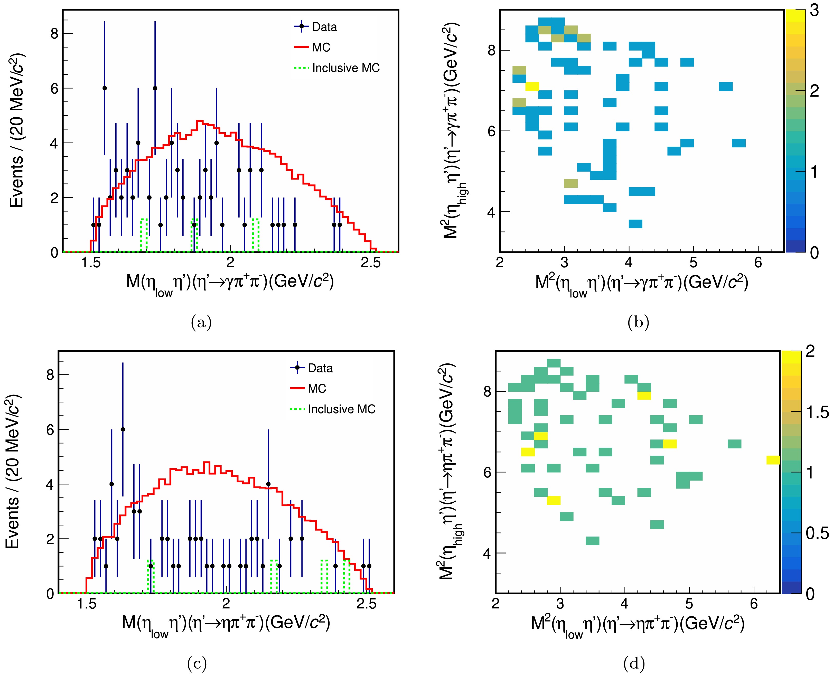
Figure 3. (color online) Invariant mass distributions and Dalitz plots for (a)(b)
$ \chi_{c1}\to\eta\eta\eta^{\prime}, \eta^{\prime}\to\gamma\pi^+\pi^- $ and (c)(d)$ \chi_{c1}\to\eta\eta\eta^{\prime}, \eta^{\prime}\to\eta\pi^+\pi^- $ . The dots with error bars are data, the red solid histograms are the signal MC, and the green dashed histograms are the inclusive MC.$ \eta_{\text{low}} $ denotes the low energy η. -
Potential backgrounds are studied using the inclusive MC samples of
$ \psi(3686) $ decays. The results show that the backgrounds can be divided into two categories: non-$ \eta^{\prime} $ processes and those containing$ \eta^{\prime} $ . Non-$ \eta^{\prime} $ backgrounds are estimated using the$ \eta^{\prime} $ mass sidebands in the data. The sideband regions of$ \eta^{\prime} $ are defined as [0.925, 0.935] and [0.98, 0.99] GeV/$ c^{2} $ . The normalization factors for events in the two sideband regions are obtained by fitting the invariant mass distributions of$ \gamma\pi^{+}\pi^{-} $ and$ \eta\pi^{+}\pi^{-} $ in the data. The$ \eta^{\prime} $ signal shapes are determined from the shapes of signal MC samples, while the$ \eta^{\prime} $ sideband shapes are described using linear functions. The backgrounds containing$ \eta^{\prime} $ are peaking backgrounds. For this type of background, the branching fractions from the PDG and efficiency obtained from background MC samples are used to estimate the normalized number of events, which is then fixed in the fit. The peaking backgrounds for the decay mode$ \eta^{\prime}\to\gamma\pi^+\pi^- $ originate from$ \chi_{c1}\to\eta J/\psi, J/\psi\to \gamma\eta\eta^{\prime} $ and$ \chi_{c1}\to\gamma J/\psi, J/\psi\to\gamma\eta\eta^{\prime} $ , with estimated yields (fractions) of 0.2 (0.2%) and 1.9 (2.6%), respectively. Similarly, the peaking backgrounds for the decay mode$ \eta^{\prime}\to\eta\pi^+\pi^- $ originate from$ \chi_{c1}\to\gamma J/\psi,\; J/\psi\to \gamma\eta\eta' $ and$ \chi_{c0}\to \eta^{\prime}\eta^{\prime} $ , with estimated yields (fractions) of 1.5 (2.6%) and 0.2 (0.3%), respectively. The background with a fraction of no more than 1.0% is neglected. -
For the two
$ \eta^{\prime} $ decay modes, there are 73 and 59 events left in the data, which are used to perform the PWA fit. The four-momenta of$ \psi(3686) $ , i.e., γ, η, η and$ \eta^{\prime} $ after the 5C kinematic fit, are used in the PWA. The decay amplitude is constructed using the helicity amplitude formalism, and the full procedure is implemented based on the open-source framework TF-PWA [33]. To construct the full decay amplitude of$ \psi(3686)\to\gamma\eta\eta\eta^{\prime} $ , the helicity formalism is used in conjunction with the isobar model, where the four-body decay is described as a two-step sequential quasi-two-body decay. For each two-body decay$ A\to B+C $ , the helicity amplitude can be written as$ A^{A\to B+C}_{\lambda_A, \lambda_B, \lambda_C} = F_{\lambda_B \lambda_C} D^{j_{A^\ast}}_{\lambda_A, \lambda_{B-C}}(\phi, \theta, 0), $

(4) where
$ D^{j_{A^\ast}}_{\lambda_A, \lambda_{B-C}}(\phi, \theta, 0) $ represents the Wigner D-function that describes the angular distribution of the final state particle with its polar (θ) and azimuthal (ϕ) angles in the rest frame of the mother particle, and$ F_{\lambda_B \lambda_C} $ represents the helicity coupling amplitude, which can be described using the LS coupling formula$ \begin{aligned}[b] F_{\lambda_B\lambda_C} = & \displaystyle\sum\limits_{ls}g_{ls}\sqrt{\dfrac{2l+1}{2J+1}}<j_B\lambda_B;j_c-\lambda_c|\mathrm{s}\delta> \\& <l0;\mathrm{s}\delta|J\delta>\left.q^lB_l^{\prime}(q,q_0,d)\right. , \end{aligned} $

(5) where
$ g_{ls} $ represents the fitting parameter;$ \lambda_{A,B,C} $ represents is the helicity of particle A, B, and C; q and$ q_0 $ represent the momentum of the invariant mass and mass of the resonance state in the rest frame, respectively; and$ B_l^{\prime}(q,q_0,d) $ represents the Blatt-Weisskopf barrier factor.The full amplitude for the complete decay chain
$ A\to R_1+B, R_1\to R_2+C, R_2\to D+E $ is constructed as the product of each two-body decay amplitude and resonant propagator$ R_1 (\chi_{c1}) $ and$ R_2 $ . The amplitude is written as Eq. 6, where$ A,B,C,D,E $ are$ \psi(3686),\gamma,\eta,\eta $ and$ \eta^{\prime} $ , respectively. The propagator R uses the relativistic Breit-Wigner formula with constant width:$BW(s) = $ $ \dfrac{1}{M^2 - s - {\rm i}\,M\Gamma}$ , where M and Γ represent the mass and width of resonances, respectively, and$ \sqrt{s} $ represents the invariant mass of$ \eta\eta^{\prime} $ or$ \eta\eta $ . Backgrounds in the PWA are estimated using normalized$ \eta^{\prime} $ sidebands and the fixed MC shape in the processes of peaking backgrounds.The construction of the PDF, calculation of the fit fraction, and corresponding statistical uncertainty for each component follow Ref. [34]. The combined branching fraction is obtained according to Eq. (7).
$ \begin{aligned}[b] A_{\lambda_A,\lambda_B',\lambda_C',\lambda_D',\lambda_E'}^{R_1,R_2} =\; & F_{{\lambda_{{R_{1}\lambda_{B}}}}}D_{{\lambda_{A},\lambda_{{R_{1}}}-\lambda_{B}}}^{{j_{{A^{*}}}}}({\boldsymbol{\varphi}}_{1},{\boldsymbol{\theta}}_{1},{\bf{0}})R_{1}({\boldsymbol{M}}) F_{{\lambda_{{R_{2}}}\lambda_{C}}}D_{{\lambda_{{R_{1}}},\lambda_{{R_{2}}}-\lambda_{C}}}^{{j_{{R_{1}^{*}}}}}({\boldsymbol{\varphi}}_{2},{\boldsymbol{\theta}}_{2},0) R_{2}({\boldsymbol{M}}) F_{{\lambda_{D}\lambda_{E}}}D_{{\lambda_{{R_{2}}},\lambda_{D}-\lambda_{E}}}^{{j_{{R_{2}^{*}}}}}({\boldsymbol{\varphi}}_{3},{\boldsymbol{\theta}}_{3},0) \\& \times D_{{\lambda_{B},\lambda_{B'}}}^{{j_{{B^{*}}}}}({\boldsymbol{\alpha}}_{B},{\boldsymbol{\beta}}_{B},{\boldsymbol{\gamma}}_{B})D_{{\lambda_{C},\lambda_{C'}}}^{{j_{{C^{*}}}}}({\boldsymbol{\alpha}}_{C},{\boldsymbol{\beta}}_{C'},{\boldsymbol{\gamma}}_{C}) D_{{\lambda_{D},\lambda_{D'}}}^{{j_{{D^{*}}}}}({\boldsymbol{\alpha}}_{D},{\boldsymbol{\beta}}_{D},{\boldsymbol{\gamma}}_{D})D_{{\lambda_{E},\lambda_{E'}}}^{{j_{{E^{*}}}}}({\boldsymbol{\alpha}}_{E},{\boldsymbol{\beta}}_{E},{\boldsymbol{\gamma}}_{E}) . \end{aligned} $

(6) -
For the two
$ \eta^{\prime} $ decay modes, there are 73 and 59 events left in the data, which are used to perform the PWA fit. The four-momenta of$ \psi(3686) $ , i.e., γ, η, η and$ \eta^{\prime} $ after the 5C kinematic fit, are used in the PWA. The decay amplitude is constructed using the helicity amplitude formalism, and the full procedure is implemented based on the open-source framework TF-PWA [33]. To construct the full decay amplitude of$ \psi(3686)\to\gamma\eta\eta\eta^{\prime} $ , the helicity formalism is used in conjunction with the isobar model, where the four-body decay is described as a two-step sequential quasi-two-body decay. For each two-body decay$ A\to B+C $ , the helicity amplitude can be written as$ A^{A\to B+C}_{\lambda_A, \lambda_B, \lambda_C} = F_{\lambda_B \lambda_C} D^{j_{A^\ast}}_{\lambda_A, \lambda_{B-C}}(\phi, \theta, 0), $
(4) where
$ D^{j_{A^\ast}}_{\lambda_A, \lambda_{B-C}}(\phi, \theta, 0) $ represents the Wigner D-function that describes the angular distribution of the final state particle with its polar (θ) and azimuthal (ϕ) angles in the rest frame of the mother particle, and$ F_{\lambda_B \lambda_C} $ represents the helicity coupling amplitude, which can be described using the LS coupling formula$ \begin{aligned}[b] F_{\lambda_B\lambda_C} = & \displaystyle\sum\limits_{ls}g_{ls}\sqrt{\dfrac{2l+1}{2J+1}}<j_B\lambda_B;j_c-\lambda_c|\mathrm{s}\delta> \\& <l0;\mathrm{s}\delta|J\delta>\left.q^lB_l^{\prime}(q,q_0,d)\right. , \end{aligned} $
(5) where
$ g_{ls} $ represents the fitting parameter;$ \lambda_{A,B,C} $ represents is the helicity of particle A, B, and C; q and$ q_0 $ represent the momentum of the invariant mass and mass of the resonance state in the rest frame, respectively; and$ B_l^{\prime}(q,q_0,d) $ represents the Blatt-Weisskopf barrier factor.The full amplitude for the complete decay chain
$ A\to R_1+B, R_1\to R_2+C, R_2\to D+E $ is constructed as the product of each two-body decay amplitude and resonant propagator$ R_1 (\chi_{c1}) $ and$ R_2 $ . The amplitude is written as Eq. 6, where$ A,B,C,D,E $ are$ \psi(3686),\gamma,\eta,\eta $ and$ \eta^{\prime} $ , respectively. The propagator R uses the relativistic Breit-Wigner formula with constant width:$BW(s) = $ $ \dfrac{1}{M^2 - s - {\rm i}\,M\Gamma}$ , where M and Γ represent the mass and width of resonances, respectively, and$ \sqrt{s} $ represents the invariant mass of$ \eta\eta^{\prime} $ or$ \eta\eta $ . Backgrounds in the PWA are estimated using normalized$ \eta^{\prime} $ sidebands and the fixed MC shape in the processes of peaking backgrounds.The construction of the PDF, calculation of the fit fraction, and corresponding statistical uncertainty for each component follow Ref. [34]. The combined branching fraction is obtained according to Eq. (7).
$ \begin{aligned}[b] A_{\lambda_A,\lambda_B',\lambda_C',\lambda_D',\lambda_E'}^{R_1,R_2} =\; & F_{{\lambda_{{R_{1}\lambda_{B}}}}}D_{{\lambda_{A},\lambda_{{R_{1}}}-\lambda_{B}}}^{{j_{{A^{*}}}}}({\boldsymbol{\varphi}}_{1},{\boldsymbol{\theta}}_{1},{\bf{0}})R_{1}({\boldsymbol{M}}) F_{{\lambda_{{R_{2}}}\lambda_{C}}}D_{{\lambda_{{R_{1}}},\lambda_{{R_{2}}}-\lambda_{C}}}^{{j_{{R_{1}^{*}}}}}({\boldsymbol{\varphi}}_{2},{\boldsymbol{\theta}}_{2},0) R_{2}({\boldsymbol{M}}) F_{{\lambda_{D}\lambda_{E}}}D_{{\lambda_{{R_{2}}},\lambda_{D}-\lambda_{E}}}^{{j_{{R_{2}^{*}}}}}({\boldsymbol{\varphi}}_{3},{\boldsymbol{\theta}}_{3},0) \\& \times D_{{\lambda_{B},\lambda_{B'}}}^{{j_{{B^{*}}}}}({\boldsymbol{\alpha}}_{B},{\boldsymbol{\beta}}_{B},{\boldsymbol{\gamma}}_{B})D_{{\lambda_{C},\lambda_{C'}}}^{{j_{{C^{*}}}}}({\boldsymbol{\alpha}}_{C},{\boldsymbol{\beta}}_{C'},{\boldsymbol{\gamma}}_{C}) D_{{\lambda_{D},\lambda_{D'}}}^{{j_{{D^{*}}}}}({\boldsymbol{\alpha}}_{D},{\boldsymbol{\beta}}_{D},{\boldsymbol{\gamma}}_{D})D_{{\lambda_{E},\lambda_{E'}}}^{{j_{{E^{*}}}}}({\boldsymbol{\alpha}}_{E},{\boldsymbol{\beta}}_{E},{\boldsymbol{\gamma}}_{E}) . \end{aligned} $
(6) -
From the mass spectrum, no obvious structure is observed in the
$ \eta\eta $ mass spectrum, whereas a structure is seen near the threshold in the mass spectrum of$ \eta\eta^{\prime} $ . Therefore, the S-wave nonresonant (NR) component and$ f_0(1500) $ in the$ \eta\eta $ mass spectrum, as well as the S-wave NR component,$ f_0(1500) $ , and$ \eta_1(1855) $ in the$ \eta\eta^{\prime} $ mass spectrum are considered. The mass and width of$ \eta_1(1855) $ are fixed at$ 1855 $ and 188 MeV/$ c^2 $ , as given in Refs. [9, 10]. The statistical significance for each component is determined by examining the change in the negative log-likelihood values when this resonance is included or excluded in the fits. The probability is calculated under the$ \chi^2 $ distribution hypothesis considering the change in the number of degrees of freedom. Resonance with a statistical significance greater than$ 5\sigma $ is included in the final set of amplitudes. The widths of the resonances in the PWA are sufficiently broad, and therefore, the effect of the detector resolution is neglected in the partial wave analysis.The results of the PWA show that the structure in the
$ \eta\eta^{\prime} $ mass spectrum is dominated by$ f_0(1500) $ with the statistical significance of$ 6.5\sigma $ , while the structure of$ \eta\eta $ is mainly described by the$ 0^{++} $ NR component. Figure 4 displays the projection plots of the fitting results of the PWA basic solution. The statistical significance of an additional$ \eta_1(1855) $ resonance is determined to be$ 0.7\sigma $ . An upper limit of branching fraction$ {\cal{B}}(\chi_{c1}\to\eta_{1}(1855)\eta) \cdot {\cal{B}}(\eta_{1}(1855)\to \eta\eta^{\prime}) $ is set. The systematic uncertainties will be described below.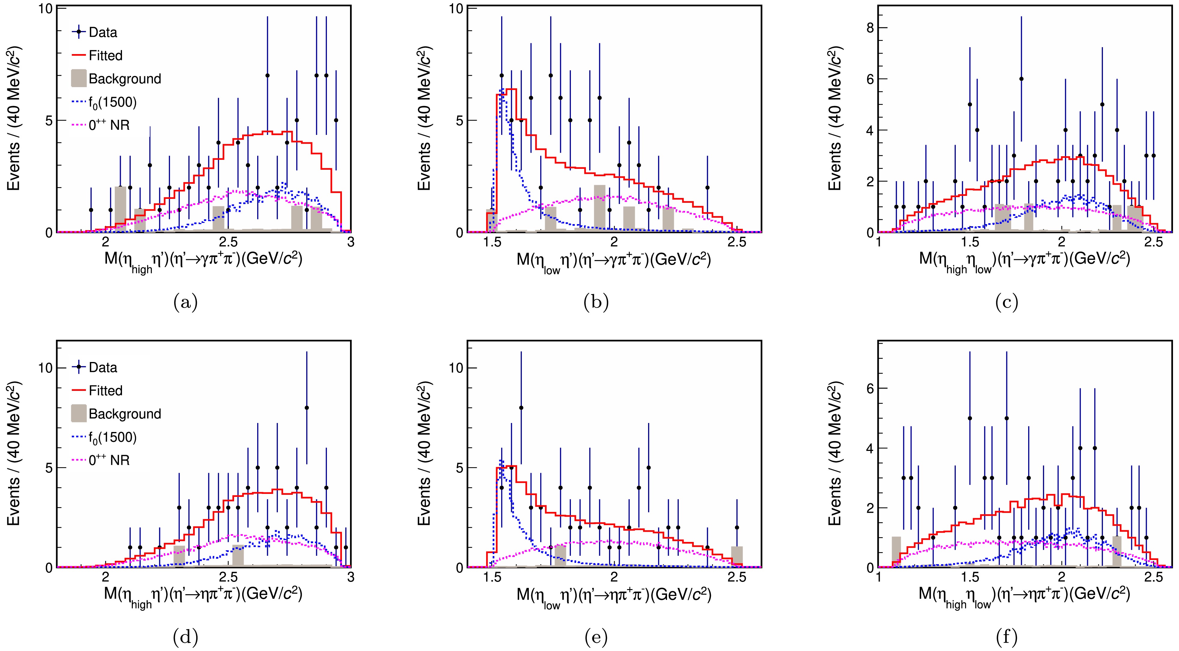
Figure 4. (color online) Data (black points with error bars) and PWA fit projections (lines) for (a)(b)(c)
$ \chi_{c1}\to\eta\eta\eta^{\prime}, \eta^{\prime}\to\gamma\pi^+\pi^- $ and (d)(e)(f)$ \chi_{c1}\to\eta\eta\eta^{\prime}, \eta^{\prime}\to\eta\pi^+\pi^- $ . The invariant mass distributions of (a)(d)$ \eta_{\text{high}}\eta^{\prime} $ , (b)(e)$ \eta_{\text{low}}\eta^{\prime} $ , and (c)(f)$ \eta_{\text{high}}\eta_{\text{low}} $ . The red solid lines are the total fit projections from the PWA, gray shadows are the background (from$ \eta^{\prime} $ sideband and peaking background), blue dashed lines represent$ f_0(1500) $ , and pink dashed lines are the$ 0^{++} $ NR components.$ \begin{aligned}[b] & {\cal{B}}(\chi_{c1}\to X\eta(\eta^{\prime}))\cdot {\cal{B}}\big(X\to\eta\eta^{\prime}(\eta\eta)\big) \\ =\;& \dfrac{N_{X_a}+N_{X_b}}{N_{\psi(3686)}\cdot {\cal{B}}(\psi(3686)\to\gamma\chi_{c1})\cdot {\cal{B}}^2(\eta\to\gamma\gamma)\cdot(\epsilon_{X_a}\cdot {\cal{B}}(\eta^{\prime}\to\gamma\pi\pi)+\epsilon_{X_b}\cdot {\cal{B}}(\eta^{\prime}\to\eta\pi\pi))\cdot {\cal{B}}\left(\eta\to\gamma\gamma\right))}. \end{aligned} $

(7) -
From the mass spectrum, no obvious structure is observed in the
$ \eta\eta $ mass spectrum, whereas a structure is seen near the threshold in the mass spectrum of$ \eta\eta^{\prime} $ . Therefore, the S-wave nonresonant (NR) component and$ f_0(1500) $ in the$ \eta\eta $ mass spectrum, as well as the S-wave NR component,$ f_0(1500) $ , and$ \eta_1(1855) $ in the$ \eta\eta^{\prime} $ mass spectrum are considered. The mass and width of$ \eta_1(1855) $ are fixed at$ 1855 $ and 188 MeV/$ c^2 $ , as given in Refs. [9, 10]. The statistical significance for each component is determined by examining the change in the negative log-likelihood values when this resonance is included or excluded in the fits. The probability is calculated under the$ \chi^2 $ distribution hypothesis considering the change in the number of degrees of freedom. Resonance with a statistical significance greater than$ 5\sigma $ is included in the final set of amplitudes. The widths of the resonances in the PWA are sufficiently broad, and therefore, the effect of the detector resolution is neglected in the partial wave analysis.The results of the PWA show that the structure in the
$ \eta\eta^{\prime} $ mass spectrum is dominated by$ f_0(1500) $ with the statistical significance of$ 6.5\sigma $ , while the structure of$ \eta\eta $ is mainly described by the$ 0^{++} $ NR component. Figure 4 displays the projection plots of the fitting results of the PWA basic solution. The statistical significance of an additional$ \eta_1(1855) $ resonance is determined to be$ 0.7\sigma $ . An upper limit of branching fraction$ {\cal{B}}(\chi_{c1}\to\eta_{1}(1855)\eta) \cdot {\cal{B}}(\eta_{1}(1855)\to \eta\eta^{\prime}) $ is set. The systematic uncertainties will be described below.
Figure 4. (color online) Data (black points with error bars) and PWA fit projections (lines) for (a)(b)(c)
$ \chi_{c1}\to\eta\eta\eta^{\prime}, \eta^{\prime}\to\gamma\pi^+\pi^- $ and (d)(e)(f)$ \chi_{c1}\to\eta\eta\eta^{\prime}, \eta^{\prime}\to\eta\pi^+\pi^- $ . The invariant mass distributions of (a)(d)$ \eta_{\text{high}}\eta^{\prime} $ , (b)(e)$ \eta_{\text{low}}\eta^{\prime} $ , and (c)(f)$ \eta_{\text{high}}\eta_{\text{low}} $ . The red solid lines are the total fit projections from the PWA, gray shadows are the background (from$ \eta^{\prime} $ sideband and peaking background), blue dashed lines represent$ f_0(1500) $ , and pink dashed lines are the$ 0^{++} $ NR components.$ \begin{aligned}[b] & {\cal{B}}(\chi_{c1}\to X\eta(\eta^{\prime}))\cdot {\cal{B}}\big(X\to\eta\eta^{\prime}(\eta\eta)\big) \\ =\;& \dfrac{N_{X_a}+N_{X_b}}{N_{\psi(3686)}\cdot {\cal{B}}(\psi(3686)\to\gamma\chi_{c1})\cdot {\cal{B}}^2(\eta\to\gamma\gamma)\cdot(\epsilon_{X_a}\cdot {\cal{B}}(\eta^{\prime}\to\gamma\pi\pi)+\epsilon_{X_b}\cdot {\cal{B}}(\eta^{\prime}\to\eta\pi\pi))\cdot {\cal{B}}\left(\eta\to\gamma\gamma\right))}. \end{aligned} $
(7) -
Systematic uncertainties are divided into two categories. The first category includes the multiplicative systematic uncertainties related to event selection, as summarized in Table 4. The second category arises from the PWA, with each alternative fit discussed below.
Independent multiplicative systematic uncertainties Source $ \gamma\pi^{+}\pi^{-} $ 

$ \eta\pi^{+}\pi^{-} $ 

Another photon reconstruction − 0.5 $ {\cal{B}}(\eta\to\gamma\gamma) $ 

− 0.5 $ {\cal{B}}(\eta^{\prime}\to\gamma(\eta)\pi^{+}\pi^{-}) $ 

1.4 1.2 Kinematic fit 0.8 0.1 $ \eta^{\prime} $ mass window

0.1 0 $ \chi_{c1} $ mass window

0.1 0 Total 1.6 1.4 Common multiplicative systematic uncertainties Source $ \gamma\pi^{+}\pi^{-} $ 

$ \eta\pi^{+}\pi^{-} $ 

$ N_{\psi(3686)} $ 

0.5 Two pion tracking 2.0 PID 2.0 Six photon reconstruction 3.0 $ {\cal{B}}(\eta\to\gamma\gamma) $ 

1.0 $ {\cal{B}}(\psi(3686)\to\gamma\chi_{c1}) $ 

2.8 Veto $ \pi^0 $ 

1.5 Total 5.3 Combined multiplicative uncertainties 5.4 Table 4. Relative multiplicative systematic uncertainties for
$ {\cal{B}}(\chi_{c1}\to\eta\eta_1(1855),\eta_1(1855)\to\eta\eta^{\prime}) $ (in %).1. Uncertainties from the
$ \eta^{\prime} $ sideband background and peaking background are treated as before.2. Uncertainty from additional resonances. To investigate the impact of other possible components on the PWA results, the
$ 0^{++} $ NR component is added to the mass spectrum of$ \eta\eta^{\prime} $ , or$ f_0(1500) $ is added to the mass spectrum of$ \eta\eta $ .3. Uncertainty from resonance parameters. In the baseline fit, the resonance parameters of the
$ \eta_1(1855) $ are fixed to PDG values [22]. An alternative fit is performed where resonance parameters are allowed to vary within one standard deviation of the PDG values, and the changes in the results are considered as systematic uncertainties.For the systematic uncertainties associated with the PWA, the maximum value of the upper limit is selected for each case. Considering multiplicative systematic uncertainties associated with event selections, the likelihood distribution is smeared using a Gaussian function with a mean of zero and a width of
$ \sigma_{\epsilon} $ , as in Eq. (3), where$ L(n) $ represents a Gaussian distribution with the mean and error from the PWA branching fraction,$ \epsilon_0 $ represents the detection efficiency obtained by PWA, and$ \sigma_{\epsilon} $ represents the combined multiplicative systematic uncertainty.$ L'(n') $ represents the smeared likelihood distribution. Taking the smearing distribution with an area of 90% as the upper limit, the result is${\cal{B}}(\chi_{c1}\to \eta_{1}(1855)\eta) \cdot {\cal{B}}(\eta_{1}(1855)\to\eta\eta^{\prime})<9.79\times 10^{-5} $ . -
Systematic uncertainties are divided into two categories. The first category includes the multiplicative systematic uncertainties related to event selection, as summarized in Table 4. The second category arises from the PWA, with each alternative fit discussed below.
Independent multiplicative systematic uncertainties Source $ \gamma\pi^{+}\pi^{-} $ $ \eta\pi^{+}\pi^{-} $ Another photon reconstruction − 0.5 $ {\cal{B}}(\eta\to\gamma\gamma) $ − 0.5 $ {\cal{B}}(\eta^{\prime}\to\gamma(\eta)\pi^{+}\pi^{-}) $ 1.4 1.2 Kinematic fit 0.8 0.1 $ \eta^{\prime} $ mass window0.1 0 $ \chi_{c1} $ mass window0.1 0 Total 1.6 1.4 Common multiplicative systematic uncertainties Source $ \gamma\pi^{+}\pi^{-} $ $ \eta\pi^{+}\pi^{-} $ $ N_{\psi(3686)} $ 0.5 Two pion tracking 2.0 PID 2.0 Six photon reconstruction 3.0 $ {\cal{B}}(\eta\to\gamma\gamma) $ 1.0 $ {\cal{B}}(\psi(3686)\to\gamma\chi_{c1}) $ 2.8 Veto $ \pi^0 $ 1.5 Total 5.3 Combined multiplicative uncertainties 5.4 Table 4. Relative multiplicative systematic uncertainties for
$ {\cal{B}}(\chi_{c1}\to\eta\eta_1(1855),\eta_1(1855)\to\eta\eta^{\prime}) $ (in %).1. Uncertainties from the
$ \eta^{\prime} $ sideband background and peaking background are treated as before.2. Uncertainty from additional resonances. To investigate the impact of other possible components on the PWA results, the
$ 0^{++} $ NR component is added to the mass spectrum of$ \eta\eta^{\prime} $ , or$ f_0(1500) $ is added to the mass spectrum of$ \eta\eta $ .3. Uncertainty from resonance parameters. In the baseline fit, the resonance parameters of the
$ \eta_1(1855) $ are fixed to PDG values [22]. An alternative fit is performed where resonance parameters are allowed to vary within one standard deviation of the PDG values, and the changes in the results are considered as systematic uncertainties.For the systematic uncertainties associated with the PWA, the maximum value of the upper limit is selected for each case. Considering multiplicative systematic uncertainties associated with event selections, the likelihood distribution is smeared using a Gaussian function with a mean of zero and a width of
$ \sigma_{\epsilon} $ , as in Eq. (3), where$ L(n) $ represents a Gaussian distribution with the mean and error from the PWA branching fraction,$ \epsilon_0 $ represents the detection efficiency obtained by PWA, and$ \sigma_{\epsilon} $ represents the combined multiplicative systematic uncertainty.$ L'(n') $ represents the smeared likelihood distribution. Taking the smearing distribution with an area of 90% as the upper limit, the result is${\cal{B}}(\chi_{c1}\to \eta_{1}(1855)\eta) \cdot {\cal{B}}(\eta_{1}(1855)\to\eta\eta^{\prime})<9.79\times 10^{-5} $ . -
The decay
$ \chi_{cJ}\to\eta\eta\eta^{\prime} $ and a PWA of$ \chi_{c1}\to\eta\eta\eta^{\prime} $ are investigated in this study based on$ 2.7\times 10^9 $ $ \psi(3686) $ events collected with the BESIII detector. The decay modes$ \chi_{c1,\, c2}\to\eta\eta\eta^{\prime} $ are observed for the first time, and their corresponding branching fractions are determined to be$ {\cal{B}}(\chi_{c1}\to\eta\eta\eta^{\prime}) = (1.40\, \pm 0.13\, (\text{stat.}) \pm 0.09\, (\text{sys.})) \times 10^{-4} $ and$ {\cal{B}}(\chi_{c2}\to\eta\eta\eta^{\prime}) = (4.18\, \pm 0.84\, (\text{stat.}) \pm 0.48\, (\text{sys.})) \times 10^{-5} $ , which are one order of magnitude lower than those of$ \chi_{c1,\, c2}\to\pi^+\pi^-\eta^{\prime} $ in PDG data [22]. An upper limit of$ 2.59 \times 10^{-5} $ at 90% CL is set for the decay$ \chi_{c0}\to\eta\eta\eta^{\prime} $ . Subsequently, a PWA of the decay$ \chi_{c1}\to\eta\eta\eta^{\prime} $ is performed to search for the$ 1^{-+} $ exotic state$ \eta_1(1855) $ . The PWA result indicates that the structure in the$ \eta\eta^{\prime} $ mass spectrum can be attributed to$ f_0(1500) $ , while in the$ \eta\eta $ mass spectrum, it is attributed to the$ 0^{++} $ NR component. No significant$ \eta_1(1855) $ is observed. The upper limit of$ {\cal{B}}(\chi_{c1}\to\eta_{1}(1855)\eta) \cdot {\cal{B}}(\eta_{1}(1855)\to\eta\eta^{\prime})< 9.79 \times 10^{-5} $ is obtained at 90% CL. In further research, the$ \eta\eta^{\prime} $ decay mode with an increased dataset and more decay modes will be explored to study$ \eta_1(1855) $ . -
The BESIII Collaboration thanks the staff of BEPCII (https://cstr.cn/31109.02.BEPC) and the IHEP computing center for their strong support.
-
The BESIII Collaboration thanks the staff of BEPCII (https://cstr.cn/31109.02.BEPC) and the IHEP computing center for their strong support.
-
The BESIII Collaboration thanks the staff of BEPCII (https://cstr.cn/31109.02.BEPC) and the IHEP computing center for their strong support.
Search for η1(1855) in χcJ → ηηη′ decays
- Received Date: 2025-04-30
- Available Online: 2025-12-15
Abstract: Based on a sample of


 DownLoad: