SU(3) flavor symmetry analysis of hyperon non-leptonic two body decays

Weak decays of hyperons have long constituted a crucial issue for testing the Standard Model (SM) and exploring new physics (NP). From the experimental side, hyperons, as intermediate states in heavy hadron cascade decay processes, are abundantly produced due to their low production threshold at many experimental facilities such as BESIII and LHCb [1−7]. Recently, BESIII has reported new measurements for the absolute branching fraction of $ \Omega^{-}\to \Xi^0\pi^{-} $, $ \Omega^{-}\to \Xi^-\pi^{0} $, $ \Omega^{-}\to \Lambda^0 K^{-} $ decay, and the sensitivity is now in the range of $ 10^{-5}\sim10^{-8} $ [8]. From the theoretical side, hyperon weak decays involve a large CKM matrix element $ V_{us}V_{ud}^* $. The precise testing of this CKM matrix element is helpful for testing the unitarity of the CKM matrix. In addition, due to their low threshold, hyperons exhibit rich non-perturbative QCD effects and distinct decay behaviors, which are reflected in their complex angular distributions [9]. In recent years, there has been much theoretical work focusing on hyperon decays such as the structure of hyperons [10], decay mechanism [11], angular distribution [12].

As for the theoretical study of the hyperon decays, strict factorization does not work well due to the low threshold and the smaller transform energy in the s quark decay modes. Therefore, the perturbative calculation is currently not feasible. Besides the perturbative study, model calculation [11, 13−16], effective theory [17−21], symmetry analysis [22−24], Lattice QCD [25, 26], and related approaches [27−29] still work well in hyperon decays. However, due to their large model independence, the uncertainty in model calculation is difficult to estimate [11]. Effective theories such as Chiral perturbation theory (χPT) have been highly successful in studying low-energy strong interaction physics. However, they may require further investigation to address the puzzle of $ \alpha(\Sigma^+\to p \gamma) $ [19]. As a symmetry analysis method, although the SU(3) analysis does not involve detailed dynamic understanding, it seems that it can solve this problem [30]. Therefore, the analysis of the hyperon decays in SU(3) symmetry is useful.

In symmetry analysis, although it is not possible to calculate the absolute values of the decay amplitudes, it can be used to obtain relations between different decay amplitudes. With a smaller number of amplitudes, when combined with experimental data, the amplitudes can be constrained and predictions can be made to further test the approach without a detailed understanding of the dynamics. Recently, there have been many symmetry analysis works on the hyperon decay processes [22−24]. As an important part of hyperon decays, hyperon non-leptonic two body decays have accumulated a large amount of experimental data and rich phenomenological observables, which have attracted considerable interest from theorists. In these processes, symmetry analyses such as isospin symmetry, which reflects the up and down quark symmetry, have been previously studied [22]. Although the isospin symmetry is powerful in hyperon non-leptonic two body weak decay processes, the SU(3) symmetry which reflects the u, d, s symmetry, requires fewer parameter and can provide more information, such as the CPV. We note that a preliminary SU(3) topological diagram analysis has been presented [23]. Unfortunately, an SU(3) symmetry analysis based on strict irreducibility representation decomposition is still absent in these processes. Therefore, further SU(3) symmetry analysis of hyperon non-leptonic two body decay processes is both necessary and urgent.

The rest of this paper is organized as follows. In Sec. II, the theoretical framework of hyperon non-leptonic two body weak decay under SU(3) symmetry is described. The decomposition of the Hamiltonian, which is the $ 3 \otimes 3 \otimes \overline{3} \otimes \overline{3} $ SU(3) group representation, is derived for the first time. In Sec. III, the octet light baryon two body decays are studied under SU(3) symmetry. Subsequently, the decuplet light baryon two body decays are analyzed in Sec. IV. Induced by the same Hamiltonian, the charmed baryon and octet light meson decay can also be studied, which are presented in Sec. V and Sec. VI, respectively. The conclusions are presented in the last section.

Under SU(3) symmetry, baryons composed of light quarks can be classified into an octet and a decuplet, while light mesons form an octet. To study the hyperon two body weak decays, the effective Hamiltonian is given as [31]

where $ V_{uq} $ is the CKM matrix element and $ z_i $ and $ y_i $ are the Wilson coefficients. For the current-current operator $ Q_{1/2} $, which is proportional to $ V_{ud}V_{us}^* $, we have $ y_{1/2}=0 $. For the penguin operator $ Q_{3-10} $, which is proportional to $ V_{td}V_{ts}^* $, we have $ z_{3-10}=0 $. To study the primary contribution of the Hamiltonian, only the tree level operators $ Q_{1} $ and $ Q_2 $ are considered in this study. These specific expressions of four-quark operator $ Q_{1/2} $ are

By extracting the flavor information, the tree level Hamiltonian can be redefined as

where $ q^{1} $, $ q^2 $, and $ q^3 $ correspond to the u, d, and s quark, respectively. The Wilson coefficient $ C_{\lambda} $ is $ z_\lambda(\mu)- \dfrac{V_{td}V_{ts}^*}{V_{ud}V_{us}^*}y_\lambda(\mu) $. The matrix $ H_\lambda $ only contains two nonzero elements, $ (H_2)^{21}_{13}=1 $ and $ (H_1)^{12}_{13}=1 $, with $ \lambda=1,2 $.

In the SU(3) irreducibility representation amplitude (IRA) method, the matrix $ H_\lambda $ can be seen as the $ 3 \otimes 3 \otimes \overline{3} \otimes \overline{3} $ SU(3) group representation, and it can be composed as $ 3 \otimes 3 \otimes \overline{3} \otimes \overline{3} = 27 \oplus 10\oplus \overline{10} \oplus 8 \oplus 8 \oplus 8 \oplus 8 \oplus 1 \oplus 1 $. In preliminary analysis, it is known that the representations 27 and $ (10 $, $ \overline {10}) $ should be the symmetric traceless representations as $ (H_{27})^{\{ij\}}_{\{kl\}} $, $ (H_{10})^{\{ijm\}} $, and $ (H_{\overline{10}})_{\{ijm\}} $. Both the traces in these representations are absorbed into the 8 and 1 representations. To construct these representation matrices, the Hamiltonian matrix $ H^{ij}_{kl} $ can be symmetrized and anti-symmetrized into four terms as follows

$ H^{\{ij\}}_{\{kl\}} $ contains the 27 representation and can be identified directly. For constructing the 10 and $ \overline{10} $ representation, the matrix can be defined as

It is evident that only index i j are symmetric in $ H^{\{ij\}m} $ and k l are symmetric in $ H_{\{kl\}n} $. After the symmetrized and anti-symmetrized processing, the complete symmetry matrix can be constructed as

with

Then, we can solve

For the last term in Eq. (4), we can extract the octet 8 and singlet 1 as

where $ \ddot{H}^n_m $ refers to the traceless octet, and its trace corresponds to a singlet. Following the same method, $ H^{\{ij\}}_{\{kl\}} $ can be decomposed into the 27, 8, and 1 representations as

where $ \tilde H^{\{ij\}}_{\{kl\}} $ is traceless. The irreducibility representation can be redefined as

Finally, the Hamiltonian matrix $ H^{ij}_{kl} $ can be decomposed by irreducibility representations as

with

Then, these irreducibility representations can be extracted as

A similar decomposition of the Hamiltonian is also employed in the analysis of tetraquarks in heavy meson weak decays [32]. After the decomposition, the specific expression of each irreducibility representation can be derived using the input Hamiltonian matrix. As the singlet is trivial, we have omitted it in the following analysis. However, it is noted that information from the Hamiltonian may provide further constraints on specific irreducibility representations. In the first step, the Hamiltonian in Eq. (3) can be redfined as $ H_+=(H_1+H_2)/2 $ and $ H_-= (H_1-H_2)/2 $. The Hamiltonian can be expressed as

where $ C_{\pm}=C_1\pm C_2 $. The index in $ H_+ $ is symmetric and $ H_- $ is anti-symmetric. This indicates that $ H_+ $ contains the $ H_{27} $, $ H_{10} $, $ H_{\overline{10}} $, and $ H^{1,2,3}_8 $ irreducibility representations. The matrix $ H_- $ only contains the $ H^4_8 $ representation. The Hamiltonian in Eq. (3) shows that the symmetry of the upper indices in $ H_\lambda $ is related to the lower indices. It can be expressed as

This suggests that $ (H_\lambda)^{ij}_{kl}=(H_\lambda)^{ji}_{lk} $. Then, we have

Therefore, $ H_{10} $, $ H_{\overline{10}} $, $ H^2_8 $, and $ H^3_8 $ are equal to zero in this study.

Under SU(3) symmetry, baryons composed of light quarks can be classified into an octet and a decuplet, while light mesons form an octet. To study the hyperon two body weak decays, the effective Hamiltonian is given as [31]

where $ V_{uq} $ is the CKM matrix element and $ z_i $ and $ y_i $ are the Wilson coefficients. For the current-current operator $ Q_{1/2} $, which is proportional to $ V_{ud}V_{us}^* $, we have $ y_{1/2}=0 $. For the penguin operator $ Q_{3-10} $, which is proportional to $ V_{td}V_{ts}^* $, we have $ z_{3-10}=0 $. To study the primary contribution of the Hamiltonian, only the tree level operators $ Q_{1} $ and $ Q_2 $ are considered in this study. These specific expressions of four-quark operator $ Q_{1/2} $ are

By extracting the flavor information, the tree level Hamiltonian can be redefined as

where $ q^{1} $, $ q^2 $, and $ q^3 $ correspond to the u, d, and s quark, respectively. The Wilson coefficient $ C_{\lambda} $ is $ z_\lambda(\mu)- \dfrac{V_{td}V_{ts}^*}{V_{ud}V_{us}^*}y_\lambda(\mu) $. The matrix $ H_\lambda $ only contains two nonzero elements, $ (H_2)^{21}_{13}=1 $ and $ (H_1)^{12}_{13}=1 $, with $ \lambda=1,2 $.

In the SU(3) irreducibility representation amplitude (IRA) method, the matrix $ H_\lambda $ can be seen as the $ 3 \otimes 3 \otimes \overline{3} \otimes \overline{3} $ SU(3) group representation, and it can be composed as $ 3 \otimes 3 \otimes \overline{3} \otimes \overline{3} = 27 \oplus 10\oplus \overline{10} \oplus 8 \oplus 8 \oplus 8 \oplus 8 \oplus 1 \oplus 1 $. In preliminary analysis, it is known that the representations 27 and $ (10 $, $ \overline {10}) $ should be the symmetric traceless representations as $ (H_{27})^{\{ij\}}_{\{kl\}} $, $ (H_{10})^{\{ijm\}} $, and $ (H_{\overline{10}})_{\{ijm\}} $. Both the traces in these representations are absorbed into the 8 and 1 representations. To construct these representation matrices, the Hamiltonian matrix $ H^{ij}_{kl} $ can be symmetrized and anti-symmetrized into four terms as follows

$ H^{\{ij\}}_{\{kl\}} $ contains the 27 representation and can be identified directly. For constructing the 10 and $ \overline{10} $ representation, the matrix can be defined as

It is evident that only index i j are symmetric in $ H^{\{ij\}m} $ and k l are symmetric in $ H_{\{kl\}n} $. After the symmetrized and anti-symmetrized processing, the complete symmetry matrix can be constructed as

with

Then, we can solve

For the last term in Eq. (4), we can extract the octet 8 and singlet 1 as

where $ \ddot{H}^n_m $ refers to the traceless octet, and its trace corresponds to a singlet. Following the same method, $ H^{\{ij\}}_{\{kl\}} $ can be decomposed into the 27, 8, and 1 representations as

where $ \tilde H^{\{ij\}}_{\{kl\}} $ is traceless. The irreducibility representation can be redefined as

Finally, the Hamiltonian matrix $ H^{ij}_{kl} $ can be decomposed by irreducibility representations as

with

Then, these irreducibility representations can be extracted as

A similar decomposition of the Hamiltonian is also employed in the analysis of tetraquarks in heavy meson weak decays [32]. After the decomposition, the specific expression of each irreducibility representation can be derived using the input Hamiltonian matrix. As the singlet is trivial, we have omitted it in the following analysis. However, it is noted that information from the Hamiltonian may provide further constraints on specific irreducibility representations. In the first step, the Hamiltonian in Eq. (3) can be redfined as $ H_+=(H_1+H_2)/2 $ and $ H_-= (H_1-H_2)/2 $. The Hamiltonian can be expressed as

where $ C_{\pm}=C_1\pm C_2 $. The index in $ H_+ $ is symmetric and $ H_- $ is anti-symmetric. This indicates that $ H_+ $ contains the $ H_{27} $, $ H_{10} $, $ H_{\overline{10}} $, and $ H^{1,2,3}_8 $ irreducibility representations. The matrix $ H_- $ only contains the $ H^4_8 $ representation. The Hamiltonian in Eq. (3) shows that the symmetry of the upper indices in $ H_\lambda $ is related to the lower indices. It can be expressed as

This suggests that $ (H_\lambda)^{ij}_{kl}=(H_\lambda)^{ji}_{lk} $. Then, we have

Therefore, $ H_{10} $, $ H_{\overline{10}} $, $ H^2_8 $, and $ H^3_8 $ are equal to zero in this study.

Using the Hamiltonian decomposition, the octet baryon two body decays $ T_8 \rightarrow T_8 P_8 $ are analyzed with the IRA method. The $ T_8 $ and $ P_8 $ respectively represent the light baryon octet and the pseudoscalar meson octet. They can be written as:

Following the analysis in Sec. II, the tree operators in Eq. (2) can be decomposed under the SU(3) flavor symmetry as $ 3 \otimes 3 \otimes \overline{3} \otimes \overline{3} = 27 \oplus 10\oplus \overline{10} \oplus 8 \oplus 8 \oplus 8 \oplus 8 \oplus 1 \oplus 1 $ and only 27 and 8 have nonzero contributions.

For the specific processes induced by $ s\rightarrow u\bar{u}d $, the Hamiltonian matrices are $ (H_{+})^{12}_{13}=(H_{+})^{21}_{13}=\dfrac{1}{2} $ and $ (H_{-})^{12}_{13}= -(H_{-})^{21}_{13}=\dfrac{1}{2} $. The representations of the IRA Hamiltonian are

Here, we define $ |V_{ud} V_{us}^*| \sim \lambda \sim \sin\theta $, which reflects the CKM factor involved in the dominant tree-level weak transition $ s \to u\bar{u}d $. This common factor is factored out from all decay amplitudes to simplify the SU(3) analysis. As $ H^1_8 $ and $ H^2_8 $ have the same contribution for the $ s\rightarrow u\bar{u}d $ transition, we only use $ H^8 $ to express these two octets. With the above expressions, one may derive the effective Hamiltonian for decays involving the octet baryon as

where $ a_{27}\sim f_{27} $ and $ a_8\sim e_8 $ are SU(3) irreducible amplitudes. The expression shows that the amplitude of octet baryon two body decays $ T_8 \rightarrow T_8 P_8 $ can be expressed by these 11 parameters. To determine these parameters, we used the experimental data presented in Table 2. Unfortunately, the current data are insufficient to determine these parameters. As each SU(3) irreducible amplitude can be divided into parity conserving and parity violating terms, the total number of the IRA method parameters is 22, which is larger than the number of observables. Therefore, in this study, the number of SU(3) irreducible amplitude is not counted correctly.

Channel	Amplitudes	Br($ 10^{-2} $)			α
		Experiment data	Our work		Experiment data	Our work
$ \Sigma^{0}\to p \pi^{-} $	$ \dfrac{{ \sin \theta } \left(5 c_8-5 d_8\right)}{20 \sqrt{2}} $	−	$ 4.713(22)\times10^{-8} $		−	$ -0.99917(20) $
$ \Sigma^{0}\to n \pi^{0} $	$ \dfrac{{ \sin \theta } \left(5 c_8+5 d_8+10 e_8\right)}{40} $	−	$ 2.340(12)\times10^{-8} $		−	$ 0.99620(47) $
$ \Lambda^{0}\to p \pi^{-} $	$ \dfrac{{ \sin \theta } \left(-10 b_8+5 c_8-8 c_{27}+5d_8-10{\bf{b^2_8}}-8{\bf{c^2_{27}}}\right)}{20 \sqrt{6}} $	$ 64.1(5) $	$ 64.1(5) $		$ 0.747(9) $	$ 0.747(9) $
$ \Lambda^{0}\to n \pi^{0} $	$ \dfrac{{ \sin \theta } \left(10 b_8-5 c_8-12 c_{27}-5d_8+10{\bf{b^2_8}}-12{\bf{c^2_{27}}}\right)}{40 \sqrt{3}} $	$ 35.9(5) $	$ 35.9(5) $		$ 0.692(17) $	$ 0.692(17) $
$ \Sigma^{+}\to p \pi^{0} $	$ \dfrac{{ \sin \theta } \left(-5 c_8+5d_8\right)}{20 \sqrt{2}} $	$ 51.47(30) $	$ 50.90(24) $		$ -0.982(14) $	$ -0.99904(22) $
$ \Sigma^{+}\to n \pi^{+} $	$ \dfrac{{ \sin \theta } \left(5 d_8+5e_8\right)}{20 } $	$ 48.43(30) $	$ 48.50(29) $		$ 0.0489(26) $	$ 0.0486(26) $
$ \Sigma^{-}\to n \pi^{-} $	$ \dfrac{{ \sin \theta } \left(5 c_8+5e_8\right)}{20} $	$ 99.848(50) $	$ 99.849(50) $		$ -0.0680(80) $	$ -0.0706(76) $
$ \Xi^{-}\to \Lambda^{0} \pi^{-} $	$ \dfrac{{ \sin \theta } \left(5a_8+5 b_8-10 c_8+4 c_{27}-10{\bf{c^2_8}}\right)}{20 \sqrt{6}} $	$ 99.887(35) $	$ 99.887(35) $		$ -0.390(7) $	$ -0.390(7) $
$ \Xi^{0}\to \Lambda^{0} \pi^{0} $	$ \dfrac{{ \sin \theta } \left(-5a_8-5 b_8+10 c_8+6c_{27}+10{\bf{c^2_8}}\right)}{40 \sqrt{3}} $	$ 99.524(12) $	$ 99.524(12) $		$ -0.349(9) $	$ -0.3490(89) $

Table 2.  Irreducible representation amplitudes (second column), experimental data (third column) and predicted values (fourth column) of the decay branching ratios, and experimental values (fifth column) and predicted values (sixth column) of the asymmetric parameters for the hyperon two-body non-leptonic decay.

By including the color information in the Hamiltonian matrix, one finds that the two quark fields or anti-quark fields in $ H^{\{ij\}}_{\{kl\}} $ are color symmetric and in $ H^{[ij]}_{[kl]} $ are anti-symmetric. As the color must be anti-symmetric in the baryon state, the amplitude in which the initial/final baryon state directly connects to the two quarks/anti-quarks in the Hamiltonian is expected to be strongly suppressed [33, 34]. To correctly count the number of SU(3) irreducible amplitudes, we can use the topological diagrammatic approach (TDA) method to provide an intuitive physical image. We find that for the color symmetric IRA Hamiltonian, only two topological diagrams (Fig. 1) can contribute. Then, the number of amplitudes of $ H_{27} $ and $ H_8^1 $ can be largely reduced. As the equivalence between the TDA and irreducible SU(3) methods has been verified [35, 36], we convert the amplitude obtained using the TDA amplitude into IRA and only write down the IRA amplitude, which includes the contributions of the two topological diagrams in Fig. 1. We find that only two amplitudes $ c_{27} $ and $ e_{27} $ correspond to these two topological diagrams. The explicit expressions of these amplitudes are given as follows: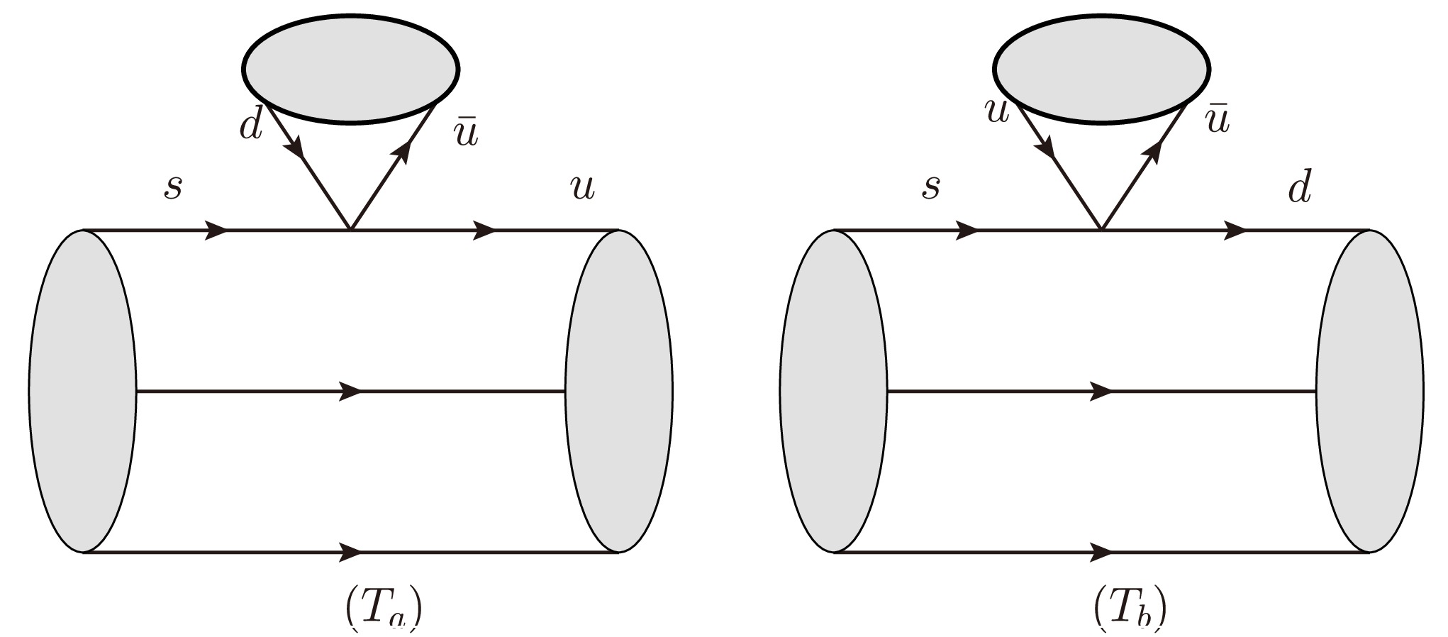

Figure 1.  Color symmetric topological diagrams for $ T_8 \rightarrow T_8P_8 $ nonleptonic decays.

We find that the contribution of $ e_{27} $ in the two amplitudes contained in the topology $ T_a $($ T_b $) is opposite. As a result, they cancel each other when the amplitudes are summed, leaving only the contribution of $ c_{27} $. Based on this simplification, the IRA amplitudes can be written as:

Although the amplitude of $ H_8^1 $ can be largely reduced, the $ H_8^4 $, which comes from the $ H^{[ij]}_{[kl]} $, will not be constrained. Therefore, the number of $ H_8 $ amplitudes remains 5. Form these amplitudes, we can derive the relations of the amplitudes by expanding them according to each decay channel in Table 2 as

In Eq. (22), there are 6 such amplitudes. In fact, these amplitudes can be expressed by 12 form factors. Generically, we can express them by parity conserving and parity violating as

For the process of octet baryon two body decays $ T_8 \rightarrow T_8P_8 $, the non-polarization decay width is easily written as

where $ \hat p_{B_n} $ is final state momentum. Depending on the specific processes, the F and G linear functions of $ f^i_{8/27} $ and $ g^i_{8/27} $ are the scalar and peseudoscalar form factors, respectively. The parameter κ writing in terms of masses is given by

Here $ M_{B_s} $, $ M_{B_n} $, and $ M_M $ are the masses of the initial octet baryons, final octet baryons, and mesons, respectively.

In this step, we find that the six SU(3) parameters cannot explain the experimental data well. However, these results are not unexpected. The hyperon decays usually involve large SU(3) symmetry breaking, considering the mass of strange quark. Therefore, in our analysis, the symmetry breaking should be considered.

As the mass of strange quark is much larger than that of the up and down quark, i.e., $ m_s $ $ \gg $ $ m_{u,d} $, the SU(3) symmetry breakdown induced by the different masses of the light u, d, and s quarks can be introduced. The quark mass matrix can be written as

The first matrix represents the mass term under the strict SU(3) symmetry and the second matrix can be seen as an interaction term, which represents the SU(3) symmetry breaking effect. Based on this mass matrix, the SU(3) symmetry-breaking contributions to the irreducible representation amplitudes can be constructed using the interaction matrix ω as:

Although 9 SU (3) symmetry breaking terms were established, we found that the degrees of freedom of our IRA amplitude are only 7.

As the decay information expressed in the SU(3) symmetry breaking terms $ {\bf{c^1_{27/8}}} $, $ {\bf{a_8}} $, $ {\bf{d_8}} $, $ {\bf{e_8}} $, and $ {\bf{b^1_8}} $ is the same as that expressed in the corresponding SU(3) symmetry terms, we can absorb these symmetry breaking contributions into the amplitude in Eq. (22). Finally, we found that only three SU(3) symmetry-breaking terms remain.

Then, one can define new parameters $ A_8 $, $ B_8 $ to absorb the symmetry breaking terms $ {\bf{b^2_8}} $ and $ {\bf{c^2_8}} $ as $ A_8=a_8-{\bf{b^2_8}}-2{\bf{c^2_8}} $, $ B_8=b_8+{\bf{b^2_8}} $. After the redefinition, the degrees of freedom are 8. Then, the amplitude $ {\bf{c_{27}}} $ contains only the symmetry breaking contributions, while the other amplitudes are contributed by both symmetry and symmetry breaking terms. Therefore, the value of $ {\bf{c_{27}}} $ represents the contribution of the symmetry breaking effect.

By the least-$ \chi^2 $ fit method[37], we can perform a global analysis of these processes.

In this study, we find that the SU(3) IRA amplitude, including symmetry breaking, can basically explain the experimental data, except the $ Br(\Sigma^{+}\to p \pi^{0} ) $ and $ \alpha(\Sigma^{+}\to p \pi^{0} ) $, which show more than 1σ deviation. By expanding the error of these two data points to 2σ, we can achieve a reasonable $ \chi^2/{\rm d.o.f}=1.54 $.

The fitting parameters and prediction results are presented in Table 1 and Table 2. For the fitted parameters in , as the available experimental data are very limited, the constraints on each fitting parameter are rather weak, and the uncertainties for parameters with comparable contributions are generally similar. However, for $ c_{27} $ and $ {\bf{c^2_{27}}} $, their contributions are relatively small, so they are less constrained by the experimental data, which leads to larger uncertainties. In particular, the contribution of $ c_{27} $ is smaller than that of $ {\bf{c^2_{27}}} $, resulting in an even larger uncertainty for $ c_{27} $. For the pseudoscalar form factors $ g_{c_{27}} $, we notice this uncertainty is much larger. Although both scalar and pseudoscalar form factors contribute to the branching ratios ($\rm Br $) and polarization parameter (α), the branching ratios are mainly determined by the scalar form factors. As a result, the pseudoscalar form factors are constrained almost exclusively by α, which also explains their relatively larger uncertainties.

parameters	Our work
	scalar(f)	pseudoscalar(g)
$ A_{8} $	$ -3.20\pm0.45 $	$ -1.74\pm0.46 $
$ B_{8} $	$ -3.32\pm0.45 $	$ -10.49\pm0.45 $
$ c_{8} $	$ -2.39\pm0.45 $	$ -8.84\pm0.45 $
$ d_{8} $	$ -3.04\pm0.45 $	$ -2.64\pm0.45 $
$ e_{8} $	$ 2.42\pm0.45 $	$ 2.48\pm0.45 $
$ c_{27} $	$ 0.0672\pm0.0010 $	$ 0.031\pm0.088 $
$ {\bf{c^2_{27}}} $	$ -0.0503\pm0.0032 $	$ -0.23\pm0.12 $
$ \chi^{2} $/d.o.f	1.54

Table 1.  SU(3) symmetry breaking irreducible amplitudes from fitting.

Our results show that the puzzle of $ {\rm Br}(\Sigma^{+}\to p \pi^{0} ) $ and $ \alpha(\Sigma^{+}\to p \pi^{0} ) $ cannot be explained by the SU(3) symmetry breaking effect. This suggests that the channel may involve a new decay mechanism, including possible contributions from new physics. We also look forward to future experiments, such as the Super Tau-Charm Facility (STCF), which can collect more data to reduce experimental errors and help resolve this puzzle. We also suggest that theorist pay more attention to this process.

To clearly see the contribution of $ H_8 $ and $ H_{27} $, and the symmetry breaking term, we can factor out the corresponding wilson coefficient as [31]

The factored form factor can be defined as

Then, one can see that the factored out SU(3) amplitudes $ c_{27}/C_+ $ and $ {\bf{c^2_{27}}}/C_+ $ are smaller than the amplitude corresponding to $ H_8 $.

However, because all amplitudes corresponding to $ H_8 $contain both symmetric and symmetry-breaking contributions, it is difficult to isolate the effects of SU(3) symmetry breaking in these channels. Fortunately, the amplitude $ {\bf{c_{27}}} $ only contains the symmetry breaking contribution. Therefore, the ratio of form factor $ R_f={\bf{f^c}}_{27}/f^c_{27} $ and $ R_g={\bf{g^c}}_{27}/g^c_{27} $ can reflect the size of symmetry breaking as $ R_f=-(75\pm5) $% and $ R_g=-(742\pm 2141) $%. We can conclude that the symmetry breaking effect in the amplitude corresponding to $ H_{27} $ is at least $ 75 $%. However, we should also note that the form factor g indicated that these processes may contain a large symmetry breaking effect of up to $ \sim1000 $%. We strongly recommend that future experimental efforts aim to reduce the measurement uncertainties, especially the processes $ \Lambda^0\to p\pi^- $ and $ \Lambda^0\to n\pi^0 $, which have larger experimental error compared to other data and play an important role in determining the parameter $ {\bf{c^2_{27}}} $. Then, the extent of SU(3) symmetry breaking can be determined with higher precision.

Using the Hamiltonian decomposition, the octet baryon two body decays $ T_8 \rightarrow T_8 P_8 $ are analyzed with the IRA method. The $ T_8 $ and $ P_8 $ respectively represent the light baryon octet and the pseudoscalar meson octet. They can be written as:

Following the analysis in Sec. II, the tree operators in Eq. (2) can be decomposed under the SU(3) flavor symmetry as $ 3 \otimes 3 \otimes \overline{3} \otimes \overline{3} = 27 \oplus 10\oplus \overline{10} \oplus 8 \oplus 8 \oplus 8 \oplus 8 \oplus 1 \oplus 1 $ and only 27 and 8 have nonzero contributions.

For the specific processes induced by $ s\rightarrow u\bar{u}d $, the Hamiltonian matrices are $ (H_{+})^{12}_{13}=(H_{+})^{21}_{13}=\dfrac{1}{2} $ and $ (H_{-})^{12}_{13}= -(H_{-})^{21}_{13}=\dfrac{1}{2} $. The representations of the IRA Hamiltonian are

Here, we define $ |V_{ud} V_{us}^*| \sim \lambda \sim \sin\theta $, which reflects the CKM factor involved in the dominant tree-level weak transition $ s \to u\bar{u}d $. This common factor is factored out from all decay amplitudes to simplify the SU(3) analysis. As $ H^1_8 $ and $ H^2_8 $ have the same contribution for the $ s\rightarrow u\bar{u}d $ transition, we only use $ H^8 $ to express these two octets. With the above expressions, one may derive the effective Hamiltonian for decays involving the octet baryon as

where $ a_{27}\sim f_{27} $ and $ a_8\sim e_8 $ are SU(3) irreducible amplitudes. The expression shows that the amplitude of octet baryon two body decays $ T_8 \rightarrow T_8 P_8 $ can be expressed by these 11 parameters. To determine these parameters, we used the experimental data presented in Table 2. Unfortunately, the current data are insufficient to determine these parameters. As each SU(3) irreducible amplitude can be divided into parity conserving and parity violating terms, the total number of the IRA method parameters is 22, which is larger than the number of observables. Therefore, in this study, the number of SU(3) irreducible amplitude is not counted correctly.

Channel	Amplitudes	Br($ 10^{-2} $)			α
		Experiment data	Our work		Experiment data	Our work
$ \Sigma^{0}\to p \pi^{-} $	$ \dfrac{{ \sin \theta } \left(5 c_8-5 d_8\right)}{20 \sqrt{2}} $	−	$ 4.713(22)\times10^{-8} $		−	$ -0.99917(20) $
$ \Sigma^{0}\to n \pi^{0} $	$ \dfrac{{ \sin \theta } \left(5 c_8+5 d_8+10 e_8\right)}{40} $	−	$ 2.340(12)\times10^{-8} $		−	$ 0.99620(47) $
$ \Lambda^{0}\to p \pi^{-} $	$ \dfrac{{ \sin \theta } \left(-10 b_8+5 c_8-8 c_{27}+5d_8-10{\bf{b^2_8}}-8{\bf{c^2_{27}}}\right)}{20 \sqrt{6}} $	$ 64.1(5) $	$ 64.1(5) $		$ 0.747(9) $	$ 0.747(9) $
$ \Lambda^{0}\to n \pi^{0} $	$ \dfrac{{ \sin \theta } \left(10 b_8-5 c_8-12 c_{27}-5d_8+10{\bf{b^2_8}}-12{\bf{c^2_{27}}}\right)}{40 \sqrt{3}} $	$ 35.9(5) $	$ 35.9(5) $		$ 0.692(17) $	$ 0.692(17) $
$ \Sigma^{+}\to p \pi^{0} $	$ \dfrac{{ \sin \theta } \left(-5 c_8+5d_8\right)}{20 \sqrt{2}} $	$ 51.47(30) $	$ 50.90(24) $		$ -0.982(14) $	$ -0.99904(22) $
$ \Sigma^{+}\to n \pi^{+} $	$ \dfrac{{ \sin \theta } \left(5 d_8+5e_8\right)}{20 } $	$ 48.43(30) $	$ 48.50(29) $		$ 0.0489(26) $	$ 0.0486(26) $
$ \Sigma^{-}\to n \pi^{-} $	$ \dfrac{{ \sin \theta } \left(5 c_8+5e_8\right)}{20} $	$ 99.848(50) $	$ 99.849(50) $		$ -0.0680(80) $	$ -0.0706(76) $
$ \Xi^{-}\to \Lambda^{0} \pi^{-} $	$ \dfrac{{ \sin \theta } \left(5a_8+5 b_8-10 c_8+4 c_{27}-10{\bf{c^2_8}}\right)}{20 \sqrt{6}} $	$ 99.887(35) $	$ 99.887(35) $		$ -0.390(7) $	$ -0.390(7) $
$ \Xi^{0}\to \Lambda^{0} \pi^{0} $	$ \dfrac{{ \sin \theta } \left(-5a_8-5 b_8+10 c_8+6c_{27}+10{\bf{c^2_8}}\right)}{40 \sqrt{3}} $	$ 99.524(12) $	$ 99.524(12) $		$ -0.349(9) $	$ -0.3490(89) $

Table 2.  Irreducible representation amplitudes (second column), experimental data (third column) and predicted values (fourth column) of the decay branching ratios, and experimental values (fifth column) and predicted values (sixth column) of the asymmetric parameters for the hyperon two-body non-leptonic decay.

By including the color information in the Hamiltonian matrix, one finds that the two quark fields or anti-quark fields in $ H^{\{ij\}}_{\{kl\}} $ are color symmetric and in $ H^{[ij]}_{[kl]} $ are anti-symmetric. As the color must be anti-symmetric in the baryon state, the amplitude in which the initial/final baryon state directly connects to the two quarks/anti-quarks in the Hamiltonian is expected to be strongly suppressed [33, 34]. To correctly count the number of SU(3) irreducible amplitudes, we can use the topological diagrammatic approach (TDA) method to provide an intuitive physical image. We find that for the color symmetric IRA Hamiltonian, only two topological diagrams (Fig. 1) can contribute. Then, the number of amplitudes of $ H_{27} $ and $ H_8^1 $ can be largely reduced. As the equivalence between the TDA and irreducible SU(3) methods has been verified [35, 36], we convert the amplitude obtained using the TDA amplitude into IRA and only write down the IRA amplitude, which includes the contributions of the two topological diagrams in Fig. 1. We find that only two amplitudes $ c_{27} $ and $ e_{27} $ correspond to these two topological diagrams. The explicit expressions of these amplitudes are given as follows:

Figure 1.  Color symmetric topological diagrams for $ T_8 \rightarrow T_8P_8 $ nonleptonic decays.

We find that the contribution of $ e_{27} $ in the two amplitudes contained in the topology $ T_a $($ T_b $) is opposite. As a result, they cancel each other when the amplitudes are summed, leaving only the contribution of $ c_{27} $. Based on this simplification, the IRA amplitudes can be written as:

Although the amplitude of $ H_8^1 $ can be largely reduced, the $ H_8^4 $, which comes from the $ H^{[ij]}_{[kl]} $, will not be constrained. Therefore, the number of $ H_8 $ amplitudes remains 5. Form these amplitudes, we can derive the relations of the amplitudes by expanding them according to each decay channel in Table 2 as

In Eq. (22), there are 6 such amplitudes. In fact, these amplitudes can be expressed by 12 form factors. Generically, we can express them by parity conserving and parity violating as

For the process of octet baryon two body decays $ T_8 \rightarrow T_8P_8 $, the non-polarization decay width is easily written as

where $ \hat p_{B_n} $ is final state momentum. Depending on the specific processes, the F and G linear functions of $ f^i_{8/27} $ and $ g^i_{8/27} $ are the scalar and peseudoscalar form factors, respectively. The parameter κ writing in terms of masses is given by

Here $ M_{B_s} $, $ M_{B_n} $, and $ M_M $ are the masses of the initial octet baryons, final octet baryons, and mesons, respectively.

In this step, we find that the six SU(3) parameters cannot explain the experimental data well. However, these results are not unexpected. The hyperon decays usually involve large SU(3) symmetry breaking, considering the mass of strange quark. Therefore, in our analysis, the symmetry breaking should be considered.

As the mass of strange quark is much larger than that of the up and down quark, i.e., $ m_s $ $ \gg $ $ m_{u,d} $, the SU(3) symmetry breakdown induced by the different masses of the light u, d, and s quarks can be introduced. The quark mass matrix can be written as

The first matrix represents the mass term under the strict SU(3) symmetry and the second matrix can be seen as an interaction term, which represents the SU(3) symmetry breaking effect. Based on this mass matrix, the SU(3) symmetry-breaking contributions to the irreducible representation amplitudes can be constructed using the interaction matrix ω as:

Although 9 SU (3) symmetry breaking terms were established, we found that the degrees of freedom of our IRA amplitude are only 7.

As the decay information expressed in the SU(3) symmetry breaking terms $ {\bf{c^1_{27/8}}} $, $ {\bf{a_8}} $, $ {\bf{d_8}} $, $ {\bf{e_8}} $, and $ {\bf{b^1_8}} $ is the same as that expressed in the corresponding SU(3) symmetry terms, we can absorb these symmetry breaking contributions into the amplitude in Eq. (22). Finally, we found that only three SU(3) symmetry-breaking terms remain.

Then, one can define new parameters $ A_8 $, $ B_8 $ to absorb the symmetry breaking terms $ {\bf{b^2_8}} $ and $ {\bf{c^2_8}} $ as $ A_8=a_8-{\bf{b^2_8}}-2{\bf{c^2_8}} $, $ B_8=b_8+{\bf{b^2_8}} $. After the redefinition, the degrees of freedom are 8. Then, the amplitude $ {\bf{c_{27}}} $ contains only the symmetry breaking contributions, while the other amplitudes are contributed by both symmetry and symmetry breaking terms. Therefore, the value of $ {\bf{c_{27}}} $ represents the contribution of the symmetry breaking effect.

By the least-$ \chi^2 $ fit method[37], we can perform a global analysis of these processes.

In this study, we find that the SU(3) IRA amplitude, including symmetry breaking, can basically explain the experimental data, except the $ Br(\Sigma^{+}\to p \pi^{0} ) $ and $ \alpha(\Sigma^{+}\to p \pi^{0} ) $, which show more than 1σ deviation. By expanding the error of these two data points to 2σ, we can achieve a reasonable $ \chi^2/{\rm d.o.f}=1.54 $.

The fitting parameters and prediction results are presented in Table 1 and Table 2. For the fitted parameters in , as the available experimental data are very limited, the constraints on each fitting parameter are rather weak, and the uncertainties for parameters with comparable contributions are generally similar. However, for $ c_{27} $ and $ {\bf{c^2_{27}}} $, their contributions are relatively small, so they are less constrained by the experimental data, which leads to larger uncertainties. In particular, the contribution of $ c_{27} $ is smaller than that of $ {\bf{c^2_{27}}} $, resulting in an even larger uncertainty for $ c_{27} $. For the pseudoscalar form factors $ g_{c_{27}} $, we notice this uncertainty is much larger. Although both scalar and pseudoscalar form factors contribute to the branching ratios ($\rm Br $) and polarization parameter (α), the branching ratios are mainly determined by the scalar form factors. As a result, the pseudoscalar form factors are constrained almost exclusively by α, which also explains their relatively larger uncertainties.

parameters	Our work
	scalar(f)	pseudoscalar(g)
$ A_{8} $	$ -3.20\pm0.45 $	$ -1.74\pm0.46 $
$ B_{8} $	$ -3.32\pm0.45 $	$ -10.49\pm0.45 $
$ c_{8} $	$ -2.39\pm0.45 $	$ -8.84\pm0.45 $
$ d_{8} $	$ -3.04\pm0.45 $	$ -2.64\pm0.45 $
$ e_{8} $	$ 2.42\pm0.45 $	$ 2.48\pm0.45 $
$ c_{27} $	$ 0.0672\pm0.0010 $	$ 0.031\pm0.088 $
$ {\bf{c^2_{27}}} $	$ -0.0503\pm0.0032 $	$ -0.23\pm0.12 $
$ \chi^{2} $/d.o.f	1.54

Table 1.  SU(3) symmetry breaking irreducible amplitudes from fitting.

Our results show that the puzzle of $ {\rm Br}(\Sigma^{+}\to p \pi^{0} ) $ and $ \alpha(\Sigma^{+}\to p \pi^{0} ) $ cannot be explained by the SU(3) symmetry breaking effect. This suggests that the channel may involve a new decay mechanism, including possible contributions from new physics. We also look forward to future experiments, such as the Super Tau-Charm Facility (STCF), which can collect more data to reduce experimental errors and help resolve this puzzle. We also suggest that theorist pay more attention to this process.

To clearly see the contribution of $ H_8 $ and $ H_{27} $, and the symmetry breaking term, we can factor out the corresponding wilson coefficient as [31]

The factored form factor can be defined as

Then, one can see that the factored out SU(3) amplitudes $ c_{27}/C_+ $ and $ {\bf{c^2_{27}}}/C_+ $ are smaller than the amplitude corresponding to $ H_8 $.

However, because all amplitudes corresponding to $ H_8 $contain both symmetric and symmetry-breaking contributions, it is difficult to isolate the effects of SU(3) symmetry breaking in these channels. Fortunately, the amplitude $ {\bf{c_{27}}} $ only contains the symmetry breaking contribution. Therefore, the ratio of form factor $ R_f={\bf{f^c}}_{27}/f^c_{27} $ and $ R_g={\bf{g^c}}_{27}/g^c_{27} $ can reflect the size of symmetry breaking as $ R_f=-(75\pm5) $% and $ R_g=-(742\pm 2141) $%. We can conclude that the symmetry breaking effect in the amplitude corresponding to $ H_{27} $ is at least $ 75 $%. However, we should also note that the form factor g indicated that these processes may contain a large symmetry breaking effect of up to $ \sim1000 $%. We strongly recommend that future experimental efforts aim to reduce the measurement uncertainties, especially the processes $ \Lambda^0\to p\pi^- $ and $ \Lambda^0\to n\pi^0 $, which have larger experimental error compared to other data and play an important role in determining the parameter $ {\bf{c^2_{27}}} $. Then, the extent of SU(3) symmetry breaking can be determined with higher precision.

Building upon the previous analysis of non-leptonic two-body decays of octet baryons, this section further extends the study to two-body decays of decuplet baryons and charmed baryons, which are induced by $ s\to d $. Although these processes involve different types of particles, the Hamiltonian can also be treated with the same method. By decomposing the effective weak Hamiltonian into irreducible representations of SU(3), we can systematically construct the amplitude structures for various decay processes.

Building upon the previous analysis of non-leptonic two-body decays of octet baryons, this section further extends the study to two-body decays of decuplet baryons and charmed baryons, which are induced by $ s\to d $. Although these processes involve different types of particles, the Hamiltonian can also be treated with the same method. By decomposing the effective weak Hamiltonian into irreducible representations of SU(3), we can systematically construct the amplitude structures for various decay processes.

The light baryons decuplet $ T_{10} $ can be written as a flavor matrix as

Using the decomposed Hamiltonian in Eq. (18), we can construct the decuplet baryon two body decays as

As the color symmetry of Hamiltonian can help us further constrain the number of independent SU(3) amplitude, as applied in octet baryon two body decays in the previous section, after considering color symmetry, the number of amplitudes corresponding to $ H_{27} $ can only be one, $ e_{27} $, and the total amplitudes are

By expanding the abovementioned expressions, we obtain the decay amplitudes listed in Table 3. Expressed by the IRA amplitude, we derive the following relations for amplitudes of decay channels as

Channel	Amplitudes
$ \Sigma^{*+}\to p\pi^{0} $	$ \dfrac{\sin \theta (-5 a_8+5b_8-5d_8+6 e_{27})}{20 \sqrt{6}} $
$ \Sigma^{*-}\to n\pi^{-} $	$ \dfrac{\sin \theta (-5 a_8-5c_8-5d_8-4 e_{27})}{20 \sqrt{3}} $
$ \Sigma^{*0}\to p\pi^{-} $	$ \dfrac{\sin \theta (-5 a_8+5b_8-5d_8-4 e_{27})}{20 \sqrt{6}} $
$ \Sigma^{*0}\to n\pi^{0} $	$ \dfrac{\sin \theta (-5 a_8-5b_8-10c_8-5d_8+6 e_{27})}{40 \sqrt{3}} $
$ \Omega^{-}\to \Xi^0\pi^{-} $	$ \dfrac{\sin \theta (5 a_8+4 e_{27})}{20} $
$ \Omega^{-}\to \Xi^-\pi^{0} $	$ \dfrac{\sin \theta (5 a_8-6 e_{27})}{20\sqrt{2}} $
$ \Xi^{*0}\to \Sigma^+\pi^{-} $	$ \dfrac{\sin \theta (5 a_8+4 e_{27})}{20\sqrt{3}} $
$ \Xi^{*0}\to \Sigma^0\pi^{0} $	$ \dfrac{\sin \theta (5 a_8-5b_8-5c_8-6 e_{27})}{40\sqrt{3}} $
$ \Xi^{*-}\to \Sigma^0\pi^{-} $	$ \dfrac{\sin \theta (-5 a_8-5b_8-5c_8-4 e_{27})}{20\sqrt{6}} $
$ \Xi^{*-}\to \Sigma^-\pi^{0} $	$ \dfrac{\sin \theta (5 a_8+5b_8+5c_8-6 e_{27})}{20\sqrt{6}} $
$ \Xi^{*0}\to \Lambda^0\pi^{0} $	$ \dfrac{\sin \theta \left(15 a_8-5b_8+5c_8+10d_8-18 e_{27}\right)}{120} $
$ \Xi^{*-}\to \Lambda^0\pi^{-} $	$ \dfrac{\sin \theta (15 a_8-5b_8+5c_8+10d_8+12 e_{27})}{60\sqrt{2}} $
$ \Xi^{*0}\to p K^{-} $	$ \dfrac{\sin\theta \left(b_8-d_8\right)}{4\sqrt{3}} $
$ \Xi^{*-}\to nK^{-} $	$ \dfrac{\sin\theta \left(-c_8-d_8\right)}{4\sqrt{3}} $
$ \Omega^{-}\to \Lambda^0 K^{-} $	$ \dfrac{\sin\theta\left(-b_8+c_8+2d_8\right)}{4\sqrt{6}} $
$ \Xi^{+}_c\to \Lambda^{+}_c\pi^{0} $	$ \dfrac{{ \sin \theta } \left(5 a_8-6 a_{27}\right)}{20 \sqrt{2}} $
$ \Xi^{0}_c\to \Lambda^{+}_c\pi^{-} $	$ \dfrac{{ \sin \theta } \left(5 a_8+4 a_{27}\right)}{20} $
$ \Xi^{'+}_c\to \Lambda^{+}_c\pi^{0} $	$ \dfrac{{ \sin \theta } \left(-5 a_8-5 b_8+6 b_{27}\right)}{40} $
$ \Xi^{'0}_c\to \Lambda^{+}_c\pi^{-} $	$ \dfrac{{ \sin \theta } \left(-5 a_8-5 b_8-4b_{27}\right)}{20\sqrt{2}} $
$ \Omega^{0}_c\to \Xi^{0}_c\pi^{0} $	$ \dfrac{{ \sin \theta } \left(5 a_8-6 b_{27}\right)}{20\sqrt{2}} $
$ \Omega^{0}_c\to \Xi^{+}_c\pi^{-} $	$ \dfrac{{ \sin \theta } \left(-5 a_8-4 b_{27}\right)}{20} $

Table 3.  Irreducible representation amplitudes of the other hyperon two-body non-leptonic decay.

The branching ratios of $ T_{10} \rightarrow T_8P_8 $ can be written as

where $ \tau_{A} $ is the lifetime of the initial decuplet baryon, $ |p_{cm}| $ is the final-state momentum in the center-of-mass frame, and $ A(T_{10A} \to T_{8B}P_{8}) $ is the decay amplitude. From the measured branching ratio $ {\cal{B}}(\Omega^{-} \to \Xi^0 \pi^{-})= (24.3\pm 0.7) $%, the decay amplitude is extracted as $ A(\Omega^{-} \to \Xi^0 \pi^{-}) = (9.66 \pm 0.15) \times 10^{-4} $. Using Eq. (35), the decay amplitude for $\Xi^{*0} \to \Sigma^+ \pi^{-} $ is derived from this result, and the corresponding branching ratio is then calculated via Eq. (36):

This branching ratio is of the order of ${\cal{O}}(10^{-14}) $, consistent with theoretical expectations. The reason lies in the different dominant interactions: the $\Omega^- $ decays primarily via weak interaction and has a relatively long lifetime of $8.21 \times 10^{-11} \mathrm{s} $, whereas $\Xi^{*0} $ decays mainly through strong interaction, leading to a much shorter lifetime on the order of ${\cal{O}}(10^{-23}) \mathrm{s} $. Consequently, the resulting branching ratio for the weak decay of $\Xi^{*0} $ is significantly suppressed, as reflected in the value obtained through Eq. (36).

We consider the two decay channels $ \Omega^{-} \to \Xi^0 \pi^{-} $ and $ \Omega^{-} \to \Xi^- \pi^{0} $ to extract the parameters $ a_8 $ and $ e_{27} $ by fitting to Eq. (25), using the corresponding branching ratios $ {\cal{B}}(\Omega^{-} \to \Xi^0 \pi^{-}) = (24.3 \pm 0.7) $%, $ {\cal{B}}(\Omega^{-} \to \Xi^- \pi^{0}) = (8.55 \pm 0.33) $%, and the symmetric parameters $ \alpha(\Omega^{-} \to \Xi^0 \pi^{-}) = 0.09 \pm 0.14 $, $ \alpha(\Omega^{-} \to \Xi^- \pi^{0}) = 0.05 \pm 0.21 $. Due to the large experimental uncertainties in the symmetric parameters α extracted from the decays $\Omega^{-} \to \Xi^0 \pi^{-} $ and $\Omega^{-} \to \Xi^- \pi^{0} $, these parameters are neglected in the present analysis. For the analysis of the decay branching ratios, we define the amplitudes in Eq. (36) for these two channels as

Then, the experimental data can be used to determine these amplitudes as

As expected from our previous discussion, the amplitude $ e_{27} $ contributes less than $ a_8 $.

With the fitted amplitude, we can make some predictions by extracting the parameter $ D_8 = -b_8 + c_8 + 2d_8 = 1.8087 \pm 0.0094 $ from the experimental data $ {\cal{B}}(\Omega^{-} \to \Lambda^0 K^{-}) = (67.7 \pm 0.7) $% using Eq. (25). This leads to the IRA amplitudes for $ \Xi^{*0} \to \Lambda^0 \pi^0 $ and $ \Xi^{*-} \to \Lambda^0 \pi^{-} $ becoming

However, due to an unknown phase angle ϕ between $ D_8 $ and $ a_8, e_{27} $, the exact amplitudes for these two decay channels cannot be determined. Our results provide the range of branching ratios for different values of the phase angle ϕ.

These predictions can be tested in future high-precision experiments.

The light baryons decuplet $ T_{10} $ can be written as a flavor matrix as

Using the decomposed Hamiltonian in Eq. (18), we can construct the decuplet baryon two body decays as

As the color symmetry of Hamiltonian can help us further constrain the number of independent SU(3) amplitude, as applied in octet baryon two body decays in the previous section, after considering color symmetry, the number of amplitudes corresponding to $ H_{27} $ can only be one, $ e_{27} $, and the total amplitudes are

By expanding the abovementioned expressions, we obtain the decay amplitudes listed in Table 3. Expressed by the IRA amplitude, we derive the following relations for amplitudes of decay channels as

Channel	Amplitudes
$ \Sigma^{*+}\to p\pi^{0} $	$ \dfrac{\sin \theta (-5 a_8+5b_8-5d_8+6 e_{27})}{20 \sqrt{6}} $
$ \Sigma^{*-}\to n\pi^{-} $	$ \dfrac{\sin \theta (-5 a_8-5c_8-5d_8-4 e_{27})}{20 \sqrt{3}} $
$ \Sigma^{*0}\to p\pi^{-} $	$ \dfrac{\sin \theta (-5 a_8+5b_8-5d_8-4 e_{27})}{20 \sqrt{6}} $
$ \Sigma^{*0}\to n\pi^{0} $	$ \dfrac{\sin \theta (-5 a_8-5b_8-10c_8-5d_8+6 e_{27})}{40 \sqrt{3}} $
$ \Omega^{-}\to \Xi^0\pi^{-} $	$ \dfrac{\sin \theta (5 a_8+4 e_{27})}{20} $
$ \Omega^{-}\to \Xi^-\pi^{0} $	$ \dfrac{\sin \theta (5 a_8-6 e_{27})}{20\sqrt{2}} $
$ \Xi^{*0}\to \Sigma^+\pi^{-} $	$ \dfrac{\sin \theta (5 a_8+4 e_{27})}{20\sqrt{3}} $
$ \Xi^{*0}\to \Sigma^0\pi^{0} $	$ \dfrac{\sin \theta (5 a_8-5b_8-5c_8-6 e_{27})}{40\sqrt{3}} $
$ \Xi^{*-}\to \Sigma^0\pi^{-} $	$ \dfrac{\sin \theta (-5 a_8-5b_8-5c_8-4 e_{27})}{20\sqrt{6}} $
$ \Xi^{*-}\to \Sigma^-\pi^{0} $	$ \dfrac{\sin \theta (5 a_8+5b_8+5c_8-6 e_{27})}{20\sqrt{6}} $
$ \Xi^{*0}\to \Lambda^0\pi^{0} $	$ \dfrac{\sin \theta \left(15 a_8-5b_8+5c_8+10d_8-18 e_{27}\right)}{120} $
$ \Xi^{*-}\to \Lambda^0\pi^{-} $	$ \dfrac{\sin \theta (15 a_8-5b_8+5c_8+10d_8+12 e_{27})}{60\sqrt{2}} $
$ \Xi^{*0}\to p K^{-} $	$ \dfrac{\sin\theta \left(b_8-d_8\right)}{4\sqrt{3}} $
$ \Xi^{*-}\to nK^{-} $	$ \dfrac{\sin\theta \left(-c_8-d_8\right)}{4\sqrt{3}} $
$ \Omega^{-}\to \Lambda^0 K^{-} $	$ \dfrac{\sin\theta\left(-b_8+c_8+2d_8\right)}{4\sqrt{6}} $
$ \Xi^{+}_c\to \Lambda^{+}_c\pi^{0} $	$ \dfrac{{ \sin \theta } \left(5 a_8-6 a_{27}\right)}{20 \sqrt{2}} $
$ \Xi^{0}_c\to \Lambda^{+}_c\pi^{-} $	$ \dfrac{{ \sin \theta } \left(5 a_8+4 a_{27}\right)}{20} $
$ \Xi^{'+}_c\to \Lambda^{+}_c\pi^{0} $	$ \dfrac{{ \sin \theta } \left(-5 a_8-5 b_8+6 b_{27}\right)}{40} $
$ \Xi^{'0}_c\to \Lambda^{+}_c\pi^{-} $	$ \dfrac{{ \sin \theta } \left(-5 a_8-5 b_8-4b_{27}\right)}{20\sqrt{2}} $
$ \Omega^{0}_c\to \Xi^{0}_c\pi^{0} $	$ \dfrac{{ \sin \theta } \left(5 a_8-6 b_{27}\right)}{20\sqrt{2}} $
$ \Omega^{0}_c\to \Xi^{+}_c\pi^{-} $	$ \dfrac{{ \sin \theta } \left(-5 a_8-4 b_{27}\right)}{20} $

Table 3.  Irreducible representation amplitudes of the other hyperon two-body non-leptonic decay.

The branching ratios of $ T_{10} \rightarrow T_8P_8 $ can be written as

where $ \tau_{A} $ is the lifetime of the initial decuplet baryon, $ |p_{cm}| $ is the final-state momentum in the center-of-mass frame, and $ A(T_{10A} \to T_{8B}P_{8}) $ is the decay amplitude. From the measured branching ratio $ {\cal{B}}(\Omega^{-} \to \Xi^0 \pi^{-})= (24.3\pm 0.7) $%, the decay amplitude is extracted as $ A(\Omega^{-} \to \Xi^0 \pi^{-}) = (9.66 \pm 0.15) \times 10^{-4} $. Using Eq. (35), the decay amplitude for $\Xi^{*0} \to \Sigma^+ \pi^{-} $ is derived from this result, and the corresponding branching ratio is then calculated via Eq. (36):

This branching ratio is of the order of ${\cal{O}}(10^{-14}) $, consistent with theoretical expectations. The reason lies in the different dominant interactions: the $\Omega^- $ decays primarily via weak interaction and has a relatively long lifetime of $8.21 \times 10^{-11} \mathrm{s} $, whereas $\Xi^{*0} $ decays mainly through strong interaction, leading to a much shorter lifetime on the order of ${\cal{O}}(10^{-23}) \mathrm{s} $. Consequently, the resulting branching ratio for the weak decay of $\Xi^{*0} $ is significantly suppressed, as reflected in the value obtained through Eq. (36).

We consider the two decay channels $ \Omega^{-} \to \Xi^0 \pi^{-} $ and $ \Omega^{-} \to \Xi^- \pi^{0} $ to extract the parameters $ a_8 $ and $ e_{27} $ by fitting to Eq. (25), using the corresponding branching ratios $ {\cal{B}}(\Omega^{-} \to \Xi^0 \pi^{-}) = (24.3 \pm 0.7) $%, $ {\cal{B}}(\Omega^{-} \to \Xi^- \pi^{0}) = (8.55 \pm 0.33) $%, and the symmetric parameters $ \alpha(\Omega^{-} \to \Xi^0 \pi^{-}) = 0.09 \pm 0.14 $, $ \alpha(\Omega^{-} \to \Xi^- \pi^{0}) = 0.05 \pm 0.21 $. Due to the large experimental uncertainties in the symmetric parameters α extracted from the decays $\Omega^{-} \to \Xi^0 \pi^{-} $ and $\Omega^{-} \to \Xi^- \pi^{0} $, these parameters are neglected in the present analysis. For the analysis of the decay branching ratios, we define the amplitudes in Eq. (36) for these two channels as

Then, the experimental data can be used to determine these amplitudes as

As expected from our previous discussion, the amplitude $ e_{27} $ contributes less than $ a_8 $.

With the fitted amplitude, we can make some predictions by extracting the parameter $ D_8 = -b_8 + c_8 + 2d_8 = 1.8087 \pm 0.0094 $ from the experimental data $ {\cal{B}}(\Omega^{-} \to \Lambda^0 K^{-}) = (67.7 \pm 0.7) $% using Eq. (25). This leads to the IRA amplitudes for $ \Xi^{*0} \to \Lambda^0 \pi^0 $ and $ \Xi^{*-} \to \Lambda^0 \pi^{-} $ becoming

However, due to an unknown phase angle ϕ between $ D_8 $ and $ a_8, e_{27} $, the exact amplitudes for these two decay channels cannot be determined. Our results provide the range of branching ratios for different values of the phase angle ϕ.

These predictions can be tested in future high-precision experiments.

Induced by the $ s\to d $ Hamiltonian, charmed baryon containing the strange quark, such as $ \{\Xi_c^{\prime+},\;\Xi_c^{\prime0}\} $, can also decay into $ \{\Xi^{+/0}_c,\;\Lambda_c\} $. Depending on whether the initial charmed baryon is an anti-triplet or a sextet baryon, the discussion can be further divided into two cases. The anti-triplet $ T_{c\overline{3}} $ and sextet $ T_{c6} $ under SU(3) flavor symmetry can be written as

Here, the SU(3) flavour anti-triplet charmed baryons can also be represented as $ (T_{c\bar 3})_i=\epsilon_{ijk}(T_{c\bar 3})^{[jk]}= (\Xi_c^0,-\Xi_c^+, \Lambda^+_c) $. Following the same method, the irreducible representation amplitudes of decay $ T_{c\bar 3} $ and $ T_{c6} $ can be constructed.

The amplitude for the two body decays of $ T_{c\overline{3}} $ is given as

To exclude the color suppressed amplitude of these processes, the TDA amplitudes are needed. The detailed discussion of TDA amplitude can be found in the appendix. A comparison with the topological diagrammatic approach (TDA) amplitudes reveals that the irreducible representation amplitudes (IRA) constructed in Eq. (43) are not subject to color suppression.

The amplitude for the two body decays of $ T_{c6} $ is given as

After excluding the color suppressed amplitude, we obtain

Expanding the above equations, we will obtain the decay amplitudes given in Table 3.

For heavy-flavor conserving decays $ \Xi^+_c \rightarrow \Lambda^+_c \pi $ and $ \Omega^0_c \rightarrow \Xi^0_c \pi $, the contribution from transition $ cs \rightarrow dc $ is also important, as $ V_{cd}V_{cs}^* \sim V_{ud}V_{us}^* \sim \sin\theta $. Within the SU(3) framework, the Hamiltonian $ H^{i}_{j} $ for the transition $ cs \rightarrow dc $ can be decomposed as

By decomposing this Hamiltonian into its irreducible representations, one obtains an octet and a singlet component. As the contribution from the singlet is negligibly small, it is not taken into account. For the octet Hamiltonian of the $ cs \rightarrow dc $ transition, the only non-zero component is $ (H_8)^2_3 = \sin\theta $. This corresponds to the non-zero component $ (H_8)^2_3 = {1}/{4} \sin\theta $ in the octet Hamiltonian of the $ s \rightarrow du\bar{u} $ transition, differing only by a coefficient. Therefore, the irreducible representation amplitude for $ cs \rightarrow dc $ can be absorbed into our existing results and does not affect our final calculations.

Induced by the $ s\to d $ Hamiltonian, charmed baryon containing the strange quark, such as $ \{\Xi_c^{\prime+},\;\Xi_c^{\prime0}\} $, can also decay into $ \{\Xi^{+/0}_c,\;\Lambda_c\} $. Depending on whether the initial charmed baryon is an anti-triplet or a sextet baryon, the discussion can be further divided into two cases. The anti-triplet $ T_{c\overline{3}} $ and sextet $ T_{c6} $ under SU(3) flavor symmetry can be written as

Here, the SU(3) flavour anti-triplet charmed baryons can also be represented as $ (T_{c\bar 3})_i=\epsilon_{ijk}(T_{c\bar 3})^{[jk]}= (\Xi_c^0,-\Xi_c^+, \Lambda^+_c) $. Following the same method, the irreducible representation amplitudes of decay $ T_{c\bar 3} $ and $ T_{c6} $ can be constructed.

The amplitude for the two body decays of $ T_{c\overline{3}} $ is given as

To exclude the color suppressed amplitude of these processes, the TDA amplitudes are needed. The detailed discussion of TDA amplitude can be found in the appendix. A comparison with the topological diagrammatic approach (TDA) amplitudes reveals that the irreducible representation amplitudes (IRA) constructed in Eq. (43) are not subject to color suppression.

The amplitude for the two body decays of $ T_{c6} $ is given as

After excluding the color suppressed amplitude, we obtain

Expanding the above equations, we will obtain the decay amplitudes given in Table 3.

For heavy-flavor conserving decays $ \Xi^+_c \rightarrow \Lambda^+_c \pi $ and $ \Omega^0_c \rightarrow \Xi^0_c \pi $, the contribution from transition $ cs \rightarrow dc $ is also important, as $ V_{cd}V_{cs}^* \sim V_{ud}V_{us}^* \sim \sin\theta $. Within the SU(3) framework, the Hamiltonian $ H^{i}_{j} $ for the transition $ cs \rightarrow dc $ can be decomposed as

By decomposing this Hamiltonian into its irreducible representations, one obtains an octet and a singlet component. As the contribution from the singlet is negligibly small, it is not taken into account. For the octet Hamiltonian of the $ cs \rightarrow dc $ transition, the only non-zero component is $ (H_8)^2_3 = \sin\theta $. This corresponds to the non-zero component $ (H_8)^2_3 = {1}/{4} \sin\theta $ in the octet Hamiltonian of the $ s \rightarrow du\bar{u} $ transition, differing only by a coefficient. Therefore, the irreducible representation amplitude for $ cs \rightarrow dc $ can be absorbed into our existing results and does not affect our final calculations.

In this work, we investigated the baryon two decay processes induced by $ s\to d \bar u u $. The hyperon two body decays with $ \Delta S=1 $ are primarily driven by this Hamiltonian, which is the central focus of our study. Under the SU(3) flavor symmetry, the baryon two body decays can be easily expressed by several IRA amplitudes. For constructing the SU(3) irreducible amplitude, the Hamiltonian corresponding to $ s\to d \bar u u $ must be decomposed as $ 3 \otimes 3 \otimes \overline{3} \otimes \overline{3} = 27 \oplus 10\oplus \overline{10} \oplus 8 \oplus 8 \oplus 8 \oplus 8 \oplus 1 \oplus 1 $. Fortunately, under the symmetric and antisymmetric transformations, the expression of each irreducible representation can be derived using Eq. (14). After including the correlation of symmetry of quark field and anti-quark field, the decuplet Hamiltonian will automatically disappear and only octet and 27-plet can contribute.

Using the decomposed Hamiltonian, we can finally construct the IRA amplitude, and by considering the color information in the baryon state and Hamiltonian, the number of independent amplitudes can be reduced to six. As we expected, the flavor symmetry is not a good symmetry in hyperon decays. Therefore, we systemically introduced a symmetry breaking effect induced by the difference of quark mass. With the symmetry breaking effect, we can perform a global analysis of the hyperon two decay processes. Our analysis shows that the $ {\rm Br}(\Sigma^{+}\to p \pi^{0} ) $ and $ \alpha(\Sigma^{+}\to p \pi^{0} ) $ deviate from our predictions by more than 1σ. This puzzle cannot be explained by the SU(3) symmetry breaking effect, suggesting potential contributions from other mechanisms. Besides, we find that the symmetry breaking effect in amplitude corresponding to $ H_{27} $ is at lest $ 75 $%, and our results indicate these processes may contain a large symmetry breaking effect of approximately $ 1000 $%. We strongly recommend that future experimental efforts aim to reduce measurement uncertainties, especially for the processes $ \Lambda^0\to p\pi^- $ and $ \Lambda^0\to n\pi^0 $, which have larger experimental errors compared to other data and play an important role in determining the parameter $ {\bf{c^2_{27}}} $. Then, the extent of SU(3) symmetry breaking can be determined with higher precision. With the help of current experiment data, we can determine part of the amplitude, and the branching ratios of $ \Xi^{*0} \to \Lambda^0 \pi^0 $ and $ \Xi^{*-} \to \Lambda^0 \pi^- $ can be estimated. However, due to the lack of experimental data, the phase of amplitude cannot be determined. Therefore, we can only provide the possible range of branching ratio in Eq. (41) by varying its phase from 0 to π. In the last part of this paper, we also analyzed the two body decays of charmed baryons induced by $ s\to d $. However, due to a lack of experimental data, we can only present the expressions for the amplitude.

In this work, we investigated the baryon two decay processes induced by $ s\to d \bar u u $. The hyperon two body decays with $ \Delta S=1 $ are primarily driven by this Hamiltonian, which is the central focus of our study. Under the SU(3) flavor symmetry, the baryon two body decays can be easily expressed by several IRA amplitudes. For constructing the SU(3) irreducible amplitude, the Hamiltonian corresponding to $ s\to d \bar u u $ must be decomposed as $ 3 \otimes 3 \otimes \overline{3} \otimes \overline{3} = 27 \oplus 10\oplus \overline{10} \oplus 8 \oplus 8 \oplus 8 \oplus 8 \oplus 1 \oplus 1 $. Fortunately, under the symmetric and antisymmetric transformations, the expression of each irreducible representation can be derived using Eq. (14). After including the correlation of symmetry of quark field and anti-quark field, the decuplet Hamiltonian will automatically disappear and only octet and 27-plet can contribute.

Using the decomposed Hamiltonian, we can finally construct the IRA amplitude, and by considering the color information in the baryon state and Hamiltonian, the number of independent amplitudes can be reduced to six. As we expected, the flavor symmetry is not a good symmetry in hyperon decays. Therefore, we systemically introduced a symmetry breaking effect induced by the difference of quark mass. With the symmetry breaking effect, we can perform a global analysis of the hyperon two decay processes. Our analysis shows that the $ {\rm Br}(\Sigma^{+}\to p \pi^{0} ) $ and $ \alpha(\Sigma^{+}\to p \pi^{0} ) $ deviate from our predictions by more than 1σ. This puzzle cannot be explained by the SU(3) symmetry breaking effect, suggesting potential contributions from other mechanisms. Besides, we find that the symmetry breaking effect in amplitude corresponding to $ H_{27} $ is at lest $ 75 $%, and our results indicate these processes may contain a large symmetry breaking effect of approximately $ 1000 $%. We strongly recommend that future experimental efforts aim to reduce measurement uncertainties, especially for the processes $ \Lambda^0\to p\pi^- $ and $ \Lambda^0\to n\pi^0 $, which have larger experimental errors compared to other data and play an important role in determining the parameter $ {\bf{c^2_{27}}} $. Then, the extent of SU(3) symmetry breaking can be determined with higher precision. With the help of current experiment data, we can determine part of the amplitude, and the branching ratios of $ \Xi^{*0} \to \Lambda^0 \pi^0 $ and $ \Xi^{*-} \to \Lambda^0 \pi^- $ can be estimated. However, due to the lack of experimental data, the phase of amplitude cannot be determined. Therefore, we can only provide the possible range of branching ratio in Eq. (41) by varying its phase from 0 to π. In the last part of this paper, we also analyzed the two body decays of charmed baryons induced by $ s\to d $. However, due to a lack of experimental data, we can only present the expressions for the amplitude.

We thank Dr. Xiao hui Hu in CUMT and Dr. Yuji Shi in ECUST for their useful discussions.

We thank Dr. Xiao hui Hu in CUMT and Dr. Yuji Shi in ECUST for their useful discussions.

In Section V, to simplify the IRA further, we also investigated the TDA of the two-body decays of charmed baryons in the anti-triplet $ T_{c\overline{3}} $ and charmed baryons in the anti-sextet $ T_{c\overline{6}} $, caused by light quarks $ s\rightarrow u\bar{u}d $. For the $ s\rightarrow u\bar{u}d $ decays, the non-zero components of the effective Hamiltonian are

The amplitudes of processes $ T_{c\overline{3}} \rightarrow T_{c\overline{3}}P_8 $ and $ T_{c\overline{6}} \rightarrow T_{c\overline{3}}P_8 $ in topological diagrammatic approach (TDA) can be written as

The relevant topological diagrams for $ T_{c\overline{3}} \rightarrow T_{c\overline{3}}P_8 $ and $ T_{c\overline{6}} \rightarrow T_{c\overline{3}}P_8 $ nonleptonic weak decays are displayed in Fig. A1. The topological diagrams in Fig. A1 can be divided into three categories: the tree diagrams in Fig. A1 (a, b), the W-exchange diagrams in Fig. A1 (c, d), and the penguin diagrams in Fig. A1 (e, f).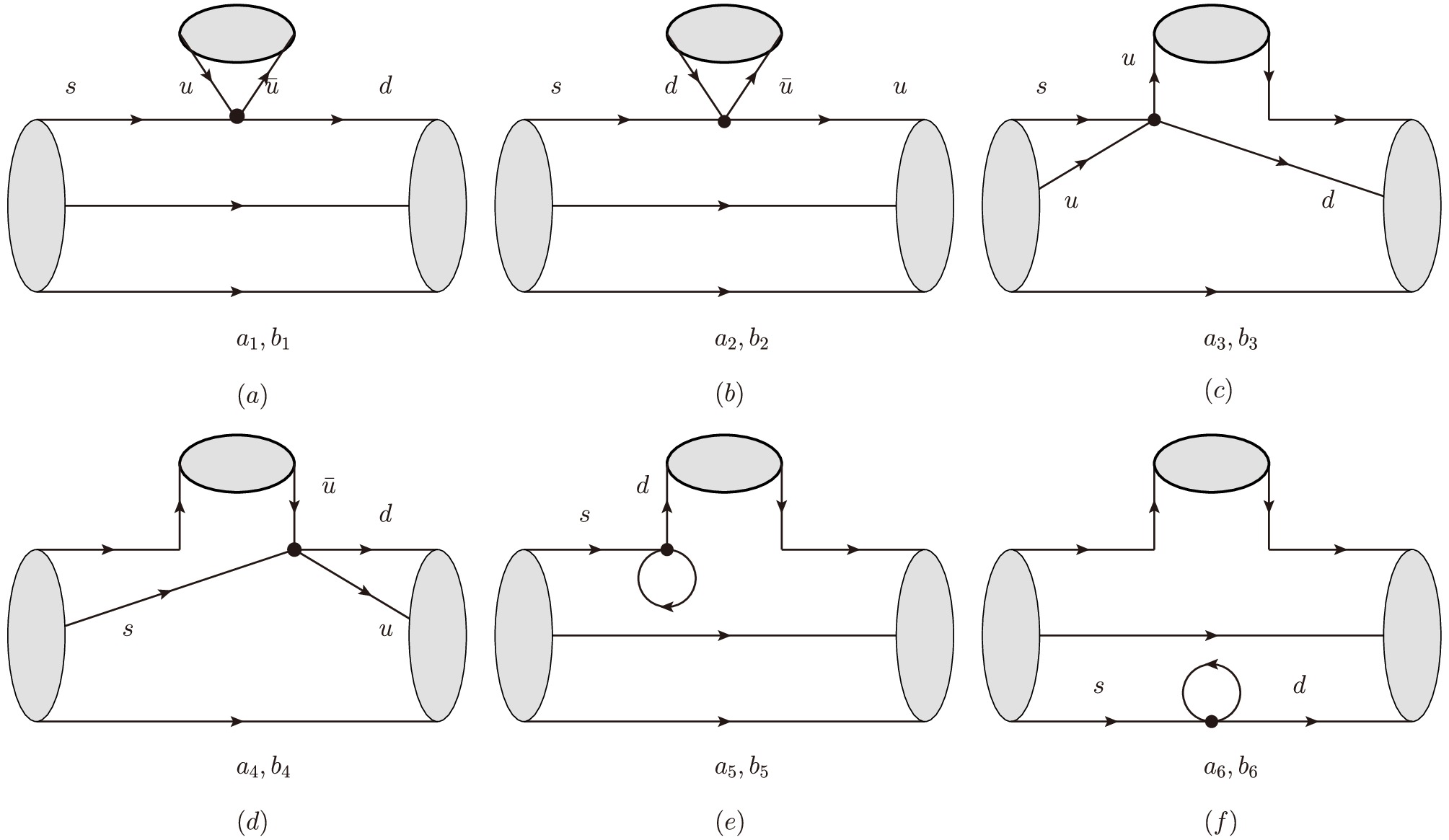

Figure A1.  Topological diagrams for $ T_{c\overline{3}} \rightarrow T_{c\overline{3}}P_8 $ and $ T_{c\overline{6}} \rightarrow $$ T_{c\overline{3}}P_8 $ nonleptonic decays.

In Section V, to simplify the IRA further, we also investigated the TDA of the two-body decays of charmed baryons in the anti-triplet $ T_{c\overline{3}} $ and charmed baryons in the anti-sextet $ T_{c\overline{6}} $, caused by light quarks $ s\rightarrow u\bar{u}d $. For the $ s\rightarrow u\bar{u}d $ decays, the non-zero components of the effective Hamiltonian are

The amplitudes of processes $ T_{c\overline{3}} \rightarrow T_{c\overline{3}}P_8 $ and $ T_{c\overline{6}} \rightarrow T_{c\overline{3}}P_8 $ in topological diagrammatic approach (TDA) can be written as

The relevant topological diagrams for $ T_{c\overline{3}} \rightarrow T_{c\overline{3}}P_8 $ and $ T_{c\overline{6}} \rightarrow T_{c\overline{3}}P_8 $ nonleptonic weak decays are displayed in Fig. A1. The topological diagrams in Fig. A1 can be divided into three categories: the tree diagrams in Fig. A1 (a, b), the W-exchange diagrams in Fig. A1 (c, d), and the penguin diagrams in Fig. A1 (e, f).

Figure A1.  Topological diagrams for $ T_{c\overline{3}} \rightarrow T_{c\overline{3}}P_8 $ and $ T_{c\overline{6}} \rightarrow $$ T_{c\overline{3}}P_8 $ nonleptonic decays.