


 Abstract
 HTML
HTML Reference
 Related
 PDF
PDF


-
The structure of nuclei with the mass number A around 130 has been a focal point of research in both nuclear physics and astrophysics. Interesting features such as the back-bending phenomenon, high-spin isomers, and γ instability in low-lying states for nuclei in this region have attracted much interest in recent years, and many results have been achieved [1−10]. Here, odd-mass nuclei with the neutron number
$ N = 79 $ exhibit a competition between the evolution of nuclear collectivity and the excitation of single-particle states, and the neutron$ h_{11/2} $ orbit plays a pivotal role in generating high-spin states. The isomeric$ 11/2_1^- $ states with neutron-hole configurations$ \nu h_{11/2}^{-1} $ have been discovered in all odd-mass$ N = 79 $ isotones, and several high-spin isomers above this$ 11/2_1^- $ state have been reported [11].A fundamental framework for describing nuclei with
$ A \sim 130 $ is the nuclear shell model (NSM) [12−17]. However, the configuration truncation is indispensable owing to the explosively increased configuration space of the NSM. The nucleon-pair approximation (NPA) [18−21] is one of the practical approaches and has been proved to be effective in studying the low-lying states of nuclei in this region [21−28]. For odd-mass$ N = 79 $ isotones, the NPA with only S and D pairs (spin equals 0 and 2) can describe the yrast states and some negative parity states below 1 MeV [24]. For higher states, pairs with higher spin should be considered.Recently, the NPA with high-spin pairs, neutron
$ (h_{11/2})^{-2} $ configuration, and several nucleon pairs with negative parity have been employed to investigate isotones with$ N = 80 $ [27]. Most calculated energy levels,$ B(E2) $ transition rates, and g factors of the low-lying states of$ ^{130} {\rm{Sn}}$ ,$ ^{132} {\rm{Te}}$ ,$ ^{134} {\rm{Xe}}$ ,$ ^{136} {\rm{Ba}}$ , and$ ^{138} {\rm{Ce}}$ are consistent with experimental values. This paper extends the approach to study the low-lying states of$ N = 79 $ isotones, i.e.,$ ^{129} {\rm{Sn}}$ ,$ ^{131} {\rm{Te}}$ ,$ ^{133} {\rm{Xe}}$ ,$ ^{135} {\rm{Ba}}$ , and$ ^{137} {\rm{Ce}}$ , and discusses the wave functions of some low-lying states in detail.The remainder of this paper is organized as follows. In Sec. II, a brief introduction to the formulation of the NPA is given, including the phenomenological Hamiltonian, nucleon-pair basis states, and electromagnetic-transition operators. The calculated results are given and discussed in Sec. III, and the summary is provided in Sec. IV. Analytical matrix elements of two-body interaction operators for odd system with one nucleon-pair are presented in Appendix A.
-
In this section, we briefly introduce the NPA, which was first developed by Chen [29] and was generalized and refined in Refs. [30−33]. In our calculations, we only consider the
$ 50 \sim 82 $ major shell with five single-particle(-hole) orbits:$ 0g_{7/2} $ ,$ 1d_{5/2} $ ,$ 1d_{3/2} $ ,$ 2s_{1/2} $ , and$ 0h_{11/2} $ . -
The Hamiltonian in this paper is similar to that in Ref. [27] and includes the spherical single-particle(-hole) energy
$ H_{0} $ , residual interactions between the like valence particles$ H_{P} $ , and quadrupole-quadrupole interactions between all valence particles$ H_{Q} $ , i.e.,$ H = H_{0} + H_{P} + H_{Q}. $

(1) The first term
$ H_{0} $ is defined as$ H_{0} = \sum\limits_{\alpha \sigma} \epsilon_{\alpha \sigma} C_{\alpha \sigma}^{\dagger} C_{\alpha \sigma}, $

(2) where
$ C_{\alpha \sigma}^{\dagger} $ ($ C_{\alpha \sigma} $ ) is a creation (an annihilation) operator, with$ \alpha = (nljm) $ denoting all the quantum numbers required for a nucleus and$ \sigma = \pi $ or ν corresponding to the proton or neutron degrees of freedom. The single-particle(-hole) energies of valence protons$ \epsilon_{j\pi} $ (valence neutron holes$ \epsilon_{j\nu} $ ) tabulated in Table 1 are obtained from experimental energies of the lowest states with spin j in$ ^{133} $ Sb ($ ^{131} {\rm{Sn}}$ ) [34−36], except$ \epsilon_{j\nu} $ for$ 1/2^{+} $ , which increases by 0.1 MeV, and for$ 11/2^{-} $ , which equals$ 0.02 + 0.01 N_{\pi} $ ($ N_{\pi} $ is the valence proton number). This adjustment is similar to those in Refs. [7, 9] and is primarily performed to reproduce the energy levels of low-lying states.$j^{{\rm{parity}}}$ 

$1/2^{+}$ 

$3/2^{+}$ 

$5/2^{+}$ 

$7/2^{+}$ 

$11/2^{-}$ 

$\epsilon_{j\pi}$ 

$2.990$ 

$2.690$ 

$0.963$ 

$0.000$ 

$2.760$ 

$\epsilon_{j\nu}$ 

$0.432$ 

$0.000$ 

$1.655$ 

$2.434$ 

ϵ Table 1. Single-particle(-hole) energies (in MeV) of valence protons (valence neutron holes) obtaineed from yrast state energies of
$^{133}{\rm{Sb}}$ ($^{131}{\rm{Sn}}$ ) [34−36], except$\epsilon_{j\nu}$ for$1/2^{+}$ ($11/2^{-}$ ), which increases by 0.1 MeV (equals ϵ). Here,$\epsilon = 0.02 + 0.01 N_{\pi}$ .The second term in Eq. (1),
$ H_{P} $ , is defined as$ H_{P} = V_{0}+V_{2}+V_{4}+V_{10}, \\ $

(3) where
$\begin{split} & V_{0} = G_{\pi}^{(0)}{\cal{P}}_{\pi}^{(0) \dagger}\cdot\widetilde{{\cal{P}}}_{\pi}^{(0)} +G_{\nu}^{(0)}{\cal{P}}_{\nu}^{(0) \dagger}\cdot\widetilde{{\cal{P}}}_{\nu}^{(0)}, \\ &V_{2} = G_{\pi}^{(2)}{\cal{P}}_{\pi}^{(2)\dagger}\cdot\widetilde{{\cal{P}}}_{\pi}^{(2)} +G_{\nu}^{(2)}{\cal{P}}_{\nu}^{(2)\dagger}\cdot\widetilde{{\cal{P}}}_{\nu}^{(2)}, \\ &V_{4} = G_{\pi}^{(4)}{\cal{P}}_{\pi}^{(4)\dagger} \cdot \widetilde{{\cal{P}}}_{\pi}^{(4)} + G_{\nu}^{(4)}{\cal{P}}_{\nu}^{(4)\dagger}\cdot\widetilde{{\cal{P}}}_{\nu}^{(4)}, \\ & V_{10} = G_{\nu}^{(10)}{\cal{P}}_{\nu}^{(10)\dagger}\cdot\widetilde{{\cal{P}}}_{\nu}^{(10)}. \end{split} $

(4) Here, the interaction parameters
$ G_{\sigma}^{(t)} $ ($ t = 0,2,4,10 $ ) of$ ^{129} {\rm{Sn}}$ ,$ ^{131} {\rm{Te}}$ ,$ ^{133} {\rm{Xe}}$ ,$ ^{135} {\rm{Ba}}$ , and$ ^{137} {\rm{Ce}}$ are tabulated in Table 2. For$ t = 0 $ ,$G_{\nu}^{(0)}$ 

$G_{\nu}^{(2)}$ 

$G_{\nu}^{(4)}$ 

$G_{\nu}^{(10)}$ 

$\kappa_{\nu}^{(2)}$ 

$-0.155-0.0015N_{\pi}$ 

$-0.019-0.00025N_{\pi}$ 

$-0.0001-0.000035N_{\pi}$ 

$0.15+0.04N_{\pi}$ 

$-0.030+0.002N_{\pi}$ 

$G_{\pi}^{(0)}$ 

$G_{\pi}^{(2)}$ 

$G_{\pi}^{(4)}$ 

$\kappa_{\pi}^{(2)}$ 

κ $-0.213+0.0015N_{\pi}$ 

$-0.029+0.0015N_{\pi}$ 

$-0.00105+0.00005N_{\pi}$ 

$-0.070+0.005N_{\pi}$ 

$0.070+0.005N_{\pi}$ 

Table 2. Interaction parameters of
$^{129}{\rm{Sn}}$ ,$^{131}{\rm{Te}}$ ,$^{133}{\rm{Xe}}$ ,$^{135}{\rm{Ba}}$ , and$^{137}{\rm{Ce}}$ .$G_{\nu}^{(0)}$ ,$G_{\pi}^{(0)}$ , and$G_{\nu}^{(10)}$ are in units of MeV,$G_{\nu}^{(4)}$ is in units of MeV/$r^{8}_{0}$ , and the others are in units of MeV/$r^{4}_{0}$ . A smooth change in these parameters with the valence proton number$N_{\pi}$ is assumed.$ \begin{split} & {\cal{P}}_{\sigma}^{(0)\dagger} = \sum\limits_{a_{\sigma}}\dfrac{\sqrt{2j_{\sigma}+1}}{2}(C_{a_{\sigma}}^{\dagger}\times C_{a_{\sigma}}^{\dagger})_{0}^{(0)}, \\ & \widetilde{{\cal{P}}}_{\sigma}^{(0)} = -\sum\limits_{a_{\sigma}}\dfrac{\sqrt{2j_{\sigma}+1}}{2}(\widetilde{C}_{a_{\sigma}}^{}\times \widetilde{C}_{a_{\sigma}}^{})_{0}^{(0)}. \end{split} $

(5) For
$ t = 2 $ and$ 4 $ ,$ \begin{split} & {\cal{P}}_{\sigma M}^{(t)\dagger} = \sum\limits_{a_{\sigma}b_{\sigma}}q(a_{\sigma}b_{\sigma}t)(C_{a_{\sigma}}^{\dagger}\times C_{b_{\sigma}}^{\dagger})_{M}^{(t)}, \\& \widetilde{{\cal{P}}}_{\sigma M}^{(t)} = -\sum\limits_{a_{\sigma}b_{\sigma}}q(a_{\sigma}b_{\sigma}t)(\widetilde{C}_{a_{\sigma}}^{}\times \widetilde{C}_{b_{\sigma}}^{})_{M}^{(t)}, \end{split}$

(6) where
$ q(ab\lambda) = -\dfrac{1}{\sqrt{2\lambda+1}}\dfrac{\langle j_{a}||r^{\lambda}Y^{\lambda}||j_{b}\rangle}{r_{0}^{\lambda}} $

(7) and
$ r_{0} $ is the oscillator parameter ($ r_{0}^{2} = 1.012A^{1/3} \; {\rm{fm}}^{2} $ ). For$ t = 10 $ ,$ {\cal{P}}_{\nu}^{(10)\dagger} = (C_{j}^{\dagger}\times C_{j}^{\dagger})_{M}^{(10)}, \; \; \; \widetilde{{\cal{P}}}_{\nu}^{(10)} = -(\widetilde{C}_{j}\times \widetilde{C}_{j})_{M}^{(10)}, $

(8) where j corresponds to the neutron
$ h_{11/2} $ orbit.The last term in Eq. (1) is
$ H_{Q} $ , which is the sum of the quadrupole-quadrupole interaction between the like valence nucleons$ V_{Q} $ and proton-neutron interaction$ V_{Q_{\pi\nu}} $ . Here,$ V_{Q} = \sum\limits_{\sigma}\kappa_{\sigma}^{(2)}Q_{\sigma}^{(2)}\cdot Q_{\sigma}^{(2)}, $

(9) $ V_{Q_{\pi\nu}} = \kappa Q_{\pi}^{(2)}\cdot Q_{\nu}^{(2)}, $

(10) with the operator
$ Q_{\sigma M}^{(2)} = \sum\limits_{ab}q(ab2)(C_{a_{\sigma}}^{\dagger}\times \widetilde{C}_{b_{\sigma}})_{M}^{(2)}, $

(11) and interaction parameters
$ \kappa_{\sigma}^{(2)} $ and κ are also given in Table 2. -
The Hamiltonian in this paper is similar to that in Ref. [27] and includes the spherical single-particle(-hole) energy
$ H_{0} $ , residual interactions between the like valence particles$ H_{P} $ , and quadrupole-quadrupole interactions between all valence particles$ H_{Q} $ , i.e.,$ H = H_{0} + H_{P} + H_{Q}. $
(1) The first term
$ H_{0} $ is defined as$ H_{0} = \sum\limits_{\alpha \sigma} \epsilon_{\alpha \sigma} C_{\alpha \sigma}^{\dagger} C_{\alpha \sigma}, $
(2) where
$ C_{\alpha \sigma}^{\dagger} $ ($ C_{\alpha \sigma} $ ) is a creation (an annihilation) operator, with$ \alpha = (nljm) $ denoting all the quantum numbers required for a nucleus and$ \sigma = \pi $ or ν corresponding to the proton or neutron degrees of freedom. The single-particle(-hole) energies of valence protons$ \epsilon_{j\pi} $ (valence neutron holes$ \epsilon_{j\nu} $ ) tabulated in Table 1 are obtained from experimental energies of the lowest states with spin j in$ ^{133} $ Sb ($ ^{131} {\rm{Sn}}$ ) [34−36], except$ \epsilon_{j\nu} $ for$ 1/2^{+} $ , which increases by 0.1 MeV, and for$ 11/2^{-} $ , which equals$ 0.02 + 0.01 N_{\pi} $ ($ N_{\pi} $ is the valence proton number). This adjustment is similar to those in Refs. [7, 9] and is primarily performed to reproduce the energy levels of low-lying states.$j^{{\rm{parity}}}$ $1/2^{+}$ $3/2^{+}$ $5/2^{+}$ $7/2^{+}$ $11/2^{-}$ $\epsilon_{j\pi}$ $2.990$ $2.690$ $0.963$ $0.000$ $2.760$ $\epsilon_{j\nu}$ $0.432$ $0.000$ $1.655$ $2.434$ ϵ Table 1. Single-particle(-hole) energies (in MeV) of valence protons (valence neutron holes) obtaineed from yrast state energies of
$^{133}{\rm{Sb}}$ ($^{131}{\rm{Sn}}$ ) [34−36], except$\epsilon_{j\nu}$ for$1/2^{+}$ ($11/2^{-}$ ), which increases by 0.1 MeV (equals ϵ). Here,$\epsilon = 0.02 + 0.01 N_{\pi}$ .The second term in Eq. (1),
$ H_{P} $ , is defined as$ H_{P} = V_{0}+V_{2}+V_{4}+V_{10}, \\ $
(3) where
$\begin{split} & V_{0} = G_{\pi}^{(0)}{\cal{P}}_{\pi}^{(0) \dagger}\cdot\widetilde{{\cal{P}}}_{\pi}^{(0)} +G_{\nu}^{(0)}{\cal{P}}_{\nu}^{(0) \dagger}\cdot\widetilde{{\cal{P}}}_{\nu}^{(0)}, \\ &V_{2} = G_{\pi}^{(2)}{\cal{P}}_{\pi}^{(2)\dagger}\cdot\widetilde{{\cal{P}}}_{\pi}^{(2)} +G_{\nu}^{(2)}{\cal{P}}_{\nu}^{(2)\dagger}\cdot\widetilde{{\cal{P}}}_{\nu}^{(2)}, \\ &V_{4} = G_{\pi}^{(4)}{\cal{P}}_{\pi}^{(4)\dagger} \cdot \widetilde{{\cal{P}}}_{\pi}^{(4)} + G_{\nu}^{(4)}{\cal{P}}_{\nu}^{(4)\dagger}\cdot\widetilde{{\cal{P}}}_{\nu}^{(4)}, \\ & V_{10} = G_{\nu}^{(10)}{\cal{P}}_{\nu}^{(10)\dagger}\cdot\widetilde{{\cal{P}}}_{\nu}^{(10)}. \end{split} $
(4) Here, the interaction parameters
$ G_{\sigma}^{(t)} $ ($ t = 0,2,4,10 $ ) of$ ^{129} {\rm{Sn}}$ ,$ ^{131} {\rm{Te}}$ ,$ ^{133} {\rm{Xe}}$ ,$ ^{135} {\rm{Ba}}$ , and$ ^{137} {\rm{Ce}}$ are tabulated in Table 2. For$ t = 0 $ ,$G_{\nu}^{(0)}$ $G_{\nu}^{(2)}$ $G_{\nu}^{(4)}$ $G_{\nu}^{(10)}$ $\kappa_{\nu}^{(2)}$ $-0.155-0.0015N_{\pi}$ $-0.019-0.00025N_{\pi}$ $-0.0001-0.000035N_{\pi}$ $0.15+0.04N_{\pi}$ $-0.030+0.002N_{\pi}$ $G_{\pi}^{(0)}$ $G_{\pi}^{(2)}$ $G_{\pi}^{(4)}$ $\kappa_{\pi}^{(2)}$ κ $-0.213+0.0015N_{\pi}$ $-0.029+0.0015N_{\pi}$ $-0.00105+0.00005N_{\pi}$ $-0.070+0.005N_{\pi}$ $0.070+0.005N_{\pi}$ Table 2. Interaction parameters of
$^{129}{\rm{Sn}}$ ,$^{131}{\rm{Te}}$ ,$^{133}{\rm{Xe}}$ ,$^{135}{\rm{Ba}}$ , and$^{137}{\rm{Ce}}$ .$G_{\nu}^{(0)}$ ,$G_{\pi}^{(0)}$ , and$G_{\nu}^{(10)}$ are in units of MeV,$G_{\nu}^{(4)}$ is in units of MeV/$r^{8}_{0}$ , and the others are in units of MeV/$r^{4}_{0}$ . A smooth change in these parameters with the valence proton number$N_{\pi}$ is assumed.$ \begin{split} & {\cal{P}}_{\sigma}^{(0)\dagger} = \sum\limits_{a_{\sigma}}\dfrac{\sqrt{2j_{\sigma}+1}}{2}(C_{a_{\sigma}}^{\dagger}\times C_{a_{\sigma}}^{\dagger})_{0}^{(0)}, \\ & \widetilde{{\cal{P}}}_{\sigma}^{(0)} = -\sum\limits_{a_{\sigma}}\dfrac{\sqrt{2j_{\sigma}+1}}{2}(\widetilde{C}_{a_{\sigma}}^{}\times \widetilde{C}_{a_{\sigma}}^{})_{0}^{(0)}. \end{split} $
(5) For
$ t = 2 $ and$ 4 $ ,$ \begin{split} & {\cal{P}}_{\sigma M}^{(t)\dagger} = \sum\limits_{a_{\sigma}b_{\sigma}}q(a_{\sigma}b_{\sigma}t)(C_{a_{\sigma}}^{\dagger}\times C_{b_{\sigma}}^{\dagger})_{M}^{(t)}, \\& \widetilde{{\cal{P}}}_{\sigma M}^{(t)} = -\sum\limits_{a_{\sigma}b_{\sigma}}q(a_{\sigma}b_{\sigma}t)(\widetilde{C}_{a_{\sigma}}^{}\times \widetilde{C}_{b_{\sigma}}^{})_{M}^{(t)}, \end{split}$
(6) where
$ q(ab\lambda) = -\dfrac{1}{\sqrt{2\lambda+1}}\dfrac{\langle j_{a}||r^{\lambda}Y^{\lambda}||j_{b}\rangle}{r_{0}^{\lambda}} $
(7) and
$ r_{0} $ is the oscillator parameter ($ r_{0}^{2} = 1.012A^{1/3} \; {\rm{fm}}^{2} $ ). For$ t = 10 $ ,$ {\cal{P}}_{\nu}^{(10)\dagger} = (C_{j}^{\dagger}\times C_{j}^{\dagger})_{M}^{(10)}, \; \; \; \widetilde{{\cal{P}}}_{\nu}^{(10)} = -(\widetilde{C}_{j}\times \widetilde{C}_{j})_{M}^{(10)}, $
(8) where j corresponds to the neutron
$ h_{11/2} $ orbit.The last term in Eq. (1) is
$ H_{Q} $ , which is the sum of the quadrupole-quadrupole interaction between the like valence nucleons$ V_{Q} $ and proton-neutron interaction$ V_{Q_{\pi\nu}} $ . Here,$ V_{Q} = \sum\limits_{\sigma}\kappa_{\sigma}^{(2)}Q_{\sigma}^{(2)}\cdot Q_{\sigma}^{(2)}, $
(9) $ V_{Q_{\pi\nu}} = \kappa Q_{\pi}^{(2)}\cdot Q_{\nu}^{(2)}, $
(10) with the operator
$ Q_{\sigma M}^{(2)} = \sum\limits_{ab}q(ab2)(C_{a_{\sigma}}^{\dagger}\times \widetilde{C}_{b_{\sigma}})_{M}^{(2)}, $
(11) and interaction parameters
$ \kappa_{\sigma}^{(2)} $ and κ are also given in Table 2. -
With the convention
$ \widetilde{C}_{jm} = (-1)^{j-m}C_{j-m} $ , a non-collective nucleon pair with spin r and projection μ, as well as its time reversal, can be defined as$ \begin{split} & A_{\mu}^{r}(ab)^{\dagger} = (C_{a}^{\dagger}\times C_{b}^{\dagger})_{\mu}^{(r)}, \\ & \widetilde{A}_{\mu}^{r}(ab) = -(\widetilde{C}_{a}\times \widetilde{C}_{b})_{\mu}^{(r)}, \end{split}$

(12) where a and b are the angular momenta of single-particle orbits. A collective nucleon pair and its time reversal can be defined as
$\begin{split} & A_{\mu}^{r\dagger} = \sum\limits_{ab}y(abr)(C_{a}^{\dagger}\times C_{b}^{\dagger})_{\mu}^{(r)}, \\& \widetilde{A}_{\mu}^{r} = -\sum\limits_{ab}y(abr) (\widetilde{C}_{a}\times \widetilde{C}_{b})_{\mu}^{(r)}, \end{split} $

(13) where the structure coefficients
$ y(abr) $ of the collective pair satisfy the symmetry$ y(abr) = (-1)^{a+b+r+1} y(bar) $

(14) and are obtained using the procedure given in Ref. [37].
For an odd system with
$ 2n+1 $ nucleons, the NPA basis state can be constructed by coupling n nucleon pairs and an unpaired nucleon in the j-orbit, i.e.,$ \begin{split} |\tau J_{n}M_{n}\rangle & \equiv A_{M_{n}}^{J_{n}\dagger}(r_{0} r_{1} \cdots r_{n}, J_{1} J_{2} \cdots J_{n}) |0\rangle \\ &= \{\cdot\cdot\cdot[(C_{j}^{\dagger}\times A^{r_{1}\dagger})^{(J_{1})} \times A^{r_{2}\dagger}]^{(J_{2})} \times \cdots \times A^{r_{n}\dagger}\}_{M_{n}}^{(J_{n})}|0\rangle, \end{split} $

(15) where
$ J_{n} $ and$ M_{n} $ are the total angular momentum and its projection of these$ 2n+1 $ nucleons, respectively, and τ represents additional necessary quantum numbers.In this paper,
$ S, D, F, G, H, I $ , and$ {\cal{J}} $ are used to represent a nucleon pair with spin 0, 2, 3, 4, 5, 6, and 7, respectively. Similar to Ref. [27], collective$ S^{+}, D^{+}, G^{+}, I^{+} $ pairs are used to construct the proton nucleon-pair basis states, expect for$ ^{137} {\rm{Ce}}$ for which collective$ S^{+}, D^{+} $ pairs and up to one$ G^{+} $ pair and one$ I^{+} $ pair are considered owing to the computational cost; collective$ S^{+}, S'^{+} $ (second spin-zero),$ D^{+}, G^{+} $ , and$ F^{-}, G^{-}, H^{-}, I^{-}, {\cal{J}}^{-} $ pairs, as well as non-collective$ (\nu h_{11/2})^{-2} $ pairs (denoted by$ {\cal{A}}_{\nu}^{(J)} $ with$ J = 2,4,6, 8,10 $ ) are taken to construct the neutron nucleon-pair basis states. The basis states in this paper are normalized but non-orthogonal to each other. -
With the convention
$ \widetilde{C}_{jm} = (-1)^{j-m}C_{j-m} $ , a non-collective nucleon pair with spin r and projection μ, as well as its time reversal, can be defined as$ \begin{split} & A_{\mu}^{r}(ab)^{\dagger} = (C_{a}^{\dagger}\times C_{b}^{\dagger})_{\mu}^{(r)}, \\ & \widetilde{A}_{\mu}^{r}(ab) = -(\widetilde{C}_{a}\times \widetilde{C}_{b})_{\mu}^{(r)}, \end{split}$
(12) where a and b are the angular momenta of single-particle orbits. A collective nucleon pair and its time reversal can be defined as
$\begin{split} & A_{\mu}^{r\dagger} = \sum\limits_{ab}y(abr)(C_{a}^{\dagger}\times C_{b}^{\dagger})_{\mu}^{(r)}, \\& \widetilde{A}_{\mu}^{r} = -\sum\limits_{ab}y(abr) (\widetilde{C}_{a}\times \widetilde{C}_{b})_{\mu}^{(r)}, \end{split} $
(13) where the structure coefficients
$ y(abr) $ of the collective pair satisfy the symmetry$ y(abr) = (-1)^{a+b+r+1} y(bar) $
(14) and are obtained using the procedure given in Ref. [37].
For an odd system with
$ 2n+1 $ nucleons, the NPA basis state can be constructed by coupling n nucleon pairs and an unpaired nucleon in the j-orbit, i.e.,$ \begin{split} |\tau J_{n}M_{n}\rangle & \equiv A_{M_{n}}^{J_{n}\dagger}(r_{0} r_{1} \cdots r_{n}, J_{1} J_{2} \cdots J_{n}) |0\rangle \\ &= \{\cdot\cdot\cdot[(C_{j}^{\dagger}\times A^{r_{1}\dagger})^{(J_{1})} \times A^{r_{2}\dagger}]^{(J_{2})} \times \cdots \times A^{r_{n}\dagger}\}_{M_{n}}^{(J_{n})}|0\rangle, \end{split} $
(15) where
$ J_{n} $ and$ M_{n} $ are the total angular momentum and its projection of these$ 2n+1 $ nucleons, respectively, and τ represents additional necessary quantum numbers.In this paper,
$ S, D, F, G, H, I $ , and$ {\cal{J}} $ are used to represent a nucleon pair with spin 0, 2, 3, 4, 5, 6, and 7, respectively. Similar to Ref. [27], collective$ S^{+}, D^{+}, G^{+}, I^{+} $ pairs are used to construct the proton nucleon-pair basis states, expect for$ ^{137} {\rm{Ce}}$ for which collective$ S^{+}, D^{+} $ pairs and up to one$ G^{+} $ pair and one$ I^{+} $ pair are considered owing to the computational cost; collective$ S^{+}, S'^{+} $ (second spin-zero),$ D^{+}, G^{+} $ , and$ F^{-}, G^{-}, H^{-}, I^{-}, {\cal{J}}^{-} $ pairs, as well as non-collective$ (\nu h_{11/2})^{-2} $ pairs (denoted by$ {\cal{A}}_{\nu}^{(J)} $ with$ J = 2,4,6, 8,10 $ ) are taken to construct the neutron nucleon-pair basis states. The basis states in this paper are normalized but non-orthogonal to each other. -
The
$ E2 $ transition operator in this paper is defined as$ T(E2) = \sum\limits_{\sigma}e_{\sigma}r_{\sigma}^{2}Y_{\sigma}^{2}, $

(16) where
$ e_{\sigma} (\sigma = \pi,\nu) $ denotes the effective charges (including bare charges) of valence protons and valence neutron holes. The$ M1 $ transition operator is defined as$ T(M1) = \sqrt{\dfrac{3}{4\pi}} \hat{\mu} = \sqrt{\dfrac{3}{4\pi}}\sum\limits_{\sigma}(g_{l\sigma}\vec{L}_{\sigma}+g_{s\sigma}\vec{S}_{\sigma}), $

(17) where
$ g_{l\sigma} $ ($ g_{s\sigma} $ ) is the orbital (spin) gyromagnetic ratios, and$ L_{\sigma} $ ($ S_{\sigma} $ ) is the total orbital angular momentum (total spin) operator. The g factor is defined as$ \mu / J $ (J is the total angular momentum), with$ \mu = \langle \Psi_{JM} | \hat{\mu}_{z} | \Psi_{JM} \rangle_{M = J}. $

(18) Similar to Ref. [27], we set
$ e_{\pi} = 1.79 $ ;$ e_{\nu} = -0.71 $ (in units of e); and$ g_{_{l\pi}} = 1.00 $ ,$ g_{_{l\nu}} = 0.02 $ ,$ g_{_{s\pi}} = 5.586 \times 0.7 $ ,$ g_{_{s\nu}} = -3.826 \times 0.7 $ (in unit of$ \mu_{N}/\hbar $ ). Here, the sign of$ e_{\nu} $ is negative because we use the hole-like picture. -
The
$ E2 $ transition operator in this paper is defined as$ T(E2) = \sum\limits_{\sigma}e_{\sigma}r_{\sigma}^{2}Y_{\sigma}^{2}, $
(16) where
$ e_{\sigma} (\sigma = \pi,\nu) $ denotes the effective charges (including bare charges) of valence protons and valence neutron holes. The$ M1 $ transition operator is defined as$ T(M1) = \sqrt{\dfrac{3}{4\pi}} \hat{\mu} = \sqrt{\dfrac{3}{4\pi}}\sum\limits_{\sigma}(g_{l\sigma}\vec{L}_{\sigma}+g_{s\sigma}\vec{S}_{\sigma}), $
(17) where
$ g_{l\sigma} $ ($ g_{s\sigma} $ ) is the orbital (spin) gyromagnetic ratios, and$ L_{\sigma} $ ($ S_{\sigma} $ ) is the total orbital angular momentum (total spin) operator. The g factor is defined as$ \mu / J $ (J is the total angular momentum), with$ \mu = \langle \Psi_{JM} | \hat{\mu}_{z} | \Psi_{JM} \rangle_{M = J}. $
(18) Similar to Ref. [27], we set
$ e_{\pi} = 1.79 $ ;$ e_{\nu} = -0.71 $ (in units of e); and$ g_{_{l\pi}} = 1.00 $ ,$ g_{_{l\nu}} = 0.02 $ ,$ g_{_{s\pi}} = 5.586 \times 0.7 $ ,$ g_{_{s\nu}} = -3.826 \times 0.7 $ (in unit of$ \mu_{N}/\hbar $ ). Here, the sign of$ e_{\nu} $ is negative because we use the hole-like picture. -
In this section, our calculated results of
$ ^{129} {\rm{Sn}}$ ,$ ^{131} {\rm{Te}}$ ,$ ^{133} {\rm{Xe}}$ ,$ ^{135} {\rm{Ba}}$ , and$ ^{137} {\rm{Ce}}$ are presented and discussed. Figure 1 and Fig. 2 present the calculated energy levels for these five$ N = 79 $ isotones, comparing them with experimental values obtained from Ref. [36]. The energy levels of most low-lying states are well reproduced. Some energy levels for which the experimental results remain inconclusive are also plotted. In addition, our calculated$ B(E2) $ transition rates (in units of W.u.) and g factors (in units of$ \mu_{N} $ ) for low-lying states are presented in Table 3 and Table 4, respectively. The corresponding experimental values [36] and some other calculations of$ B(E2) $ [3, 9, 28, 38, 39] and g factors [9, 24, 28, 40, 41] are also given for comparison. Our calculated$ B(E2) $ and g factors show reasonable agreement with experimental values.
Figure 1. Energy levels of
$^{129}{\rm{Sn}}$ . The left-hand (right-hand) side corresponds to experimental values [36] (our NPA calculated results).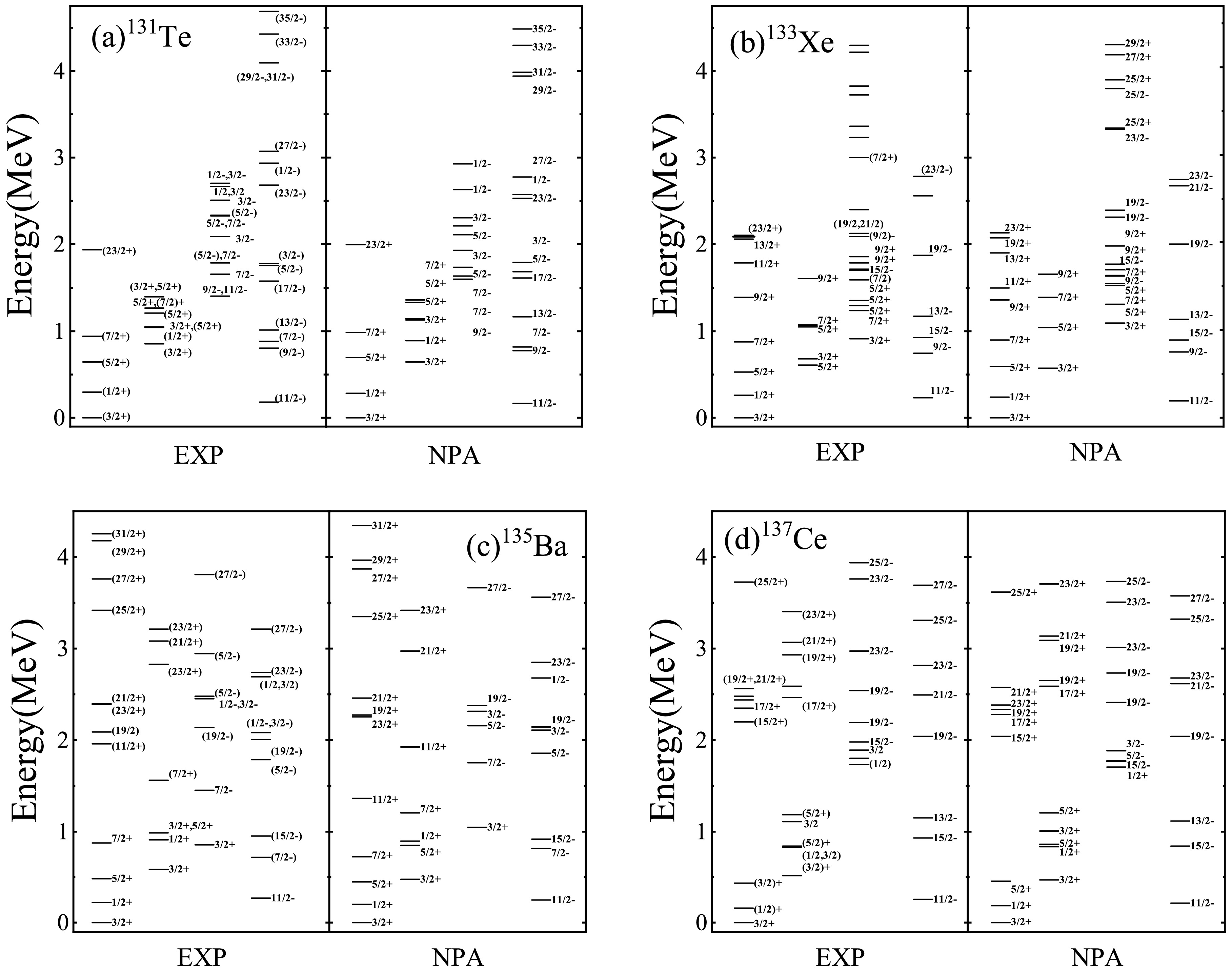
Figure 2. Same as Fig. 1. Panels (a), (b), (c), and (d) correspond to
$^{131}{\rm{Te}}$ ,$^{133}{\rm{Xe}}$ ,$^{135}{\rm{Ba}}$ , and$^{137}{\rm{Ce}}$ , respectively.$J_{i}\to J_{f}$ 

$B(E2)$ 

NPA Others Expt. $^{129}{\rm{Sn}}$ 

$3/2_{1}^{+}\to1/2_{1}^{+}$ 

0.758 1.11a – $5/2_{1}^{+}\to3/2_{1}^{+}$ 

1.54 1.88a – $5/2_{1}^{+}\to1/2_{1}^{+}$ 

0.272 0.0328a – $19/2_{1}^{+}\to15/2_{1}^{+}$ 

1.38 1.39a/0.83b 1.4(6) $23/2_{1}^{+}\to19/2_{1}^{+}$ 

0.829 0.633a/0.58b 1.39(10) $9/2_{1}^{-}\to11/2_{1}^{-}$ 

1.87 3.02a – $7/2_{1}^{-}\to11/2_{1}^{-}$ 

1.72 1.97a – $7/2_{1}^{-}\to9/2_{1}^{-}$ 

1.01 0.169a – $15/2_{1}^{-}\to11/2_{1}^{-}$ 

1.69 0.97b 1.12(34) $27/2_{1}^{-}\to23/2_{1}^{-}$ 

0.561 0.565c 0.79(36) $^{131}{\rm{Te}}$ 

$1/2_{1}^{+}\to3/2_{1}^{+}$ 

2.63 8.23a – $5/2_{1}^{+}\to3/2_{1}^{+}$ 

5.97 7.92a – $5/2_{1}^{+}\to1/2_{1}^{+}$ 

0.739 0.0212a – $7/2_{1}^{+}\to3/2_{1}^{+}$ 

6.20 8.40a 10.17d $9/2_{1}^{-}\to11/2_{1}^{-}$ 

6.19 8.99a – $7/2_{1}^{-}\to9/2_{1}^{-}$ 

3.46 1.25a – $7/2_{1}^{-}\to11/2_{1}^{-}$ 

6.95 7.83a – $15/2_{1}^{-}\to11/2_{1}^{-}$ 

7.11 12.70d – $13/2_{1}^{-}\to11/2_{1}^{-}$ 

7.6 8.125e – $17/2_{1}^{-}\to13/2_{1}^{-}$ 

2.95 3.07a/2.37d/2.255e 3.5 $19/2_{1}^{-}\to15/2_{1}^{-}$ 

5.51 4.24d – $23/2_{1}^{-}\to19/2_{1}^{-}$ 

7.69 1.88d – $^{133}{\rm{Xe}}$ 

$1/2_{1}^{+}\to3/2_{1}^{+}$ 

6.04 15.1a – $5/2_{1}^{+}\to3/2_{1}^{+}$ 

13.74 19.9a – $7/2_{1}^{+}\to3/2_{1}^{+}$ 

11.81 17.5a – $9/2_{1}^{-}\to11/2_{1}^{-}$ 

10.9 15.2a – $15/2_{1}^{-}\to11/2_{1}^{-}$ 

10.6 13.8a – $^{135}{\rm{Ba}}$ 

$1/2_{1}^{+}\to3/2_{1}^{+}$ 

11.7 16.2a 4.6(2) $1/2_{2}^{+}\to3/2_{1}^{+}$ 

6.43 2.21a 11.7(10) $3/2_{2}^{+}\to3/2_{1}^{+}$ 

17.04 10.9a 18(10) $5/2_{1}^{+}\to1/2_{1}^{+}$ 

2.55 1.31a 2.6(5) $5/2_{1}^{+}\to3/2_{1}^{+}$ 

30.63 37.2a 28.3(10) $7/2_{1}^{+}\to3/2_{1}^{+}$ 

21.5 25.0a 19.9(8) $^{137}{\rm{Ce}}$ 

$1/2_{1}^{+}\to3/2_{1}^{+}$ 

12.46 – – $3/2_{2}^{+}\to3/2_{1}^{+}$ 

18.16 – – $15/2_{1}^{-}\to11/2_{1}^{-}$ 

16.98 – – $9/2_{1}^{-}\to11/2_{1}^{-}$ 

15.83 – – $9/2_{1}^{-}\to7/2_{1}^{-}$ 

12.04 – – $13/2_{1}^{-}\to9/2_{1}^{-}$ 

0.214 – – Table 3.
$B(E2)$ values (in units of W.u.) of$^{129}{\rm{Sn}}$ ,$^{131}{\rm{Te}}$ ,$^{133}{\rm{Xe}}$ ,$^{135}{\rm{Ba}}$ , and$^{137}{\rm{Ce}}$ . Some experimental values [36] and theoretical results obtained from aRef. [9], bRef. [39], cRef. [38], dRef. [28], and eRef. [3] are also given for comparison.J $g$ factor

NPA Others Expt. $^{129}{\rm{Sn}}$ 

$3/2_{1}^{+}$ 

0.806 0.803a/0.817b/0.761c 0.754(6) $1/2_{1}^{+}$ 

−1.234 −1.250c – $5/2_{1}^{+}$ 

0.129 0.116a/0.06c – $7/2_{1}^{-}$ 

−1.134 −0.899a – $9/2_{1}^{-}$ 

−1.067 −1.11a/−1.152c – $11/2_{1}^{-}$ 

−1.238 −1.34a/−1.264b/−1.337c −1.297(5) $^{131}{\rm{Te}}$ 

$3/2_{1}^{+}$ 

0.833 0.843a/0.773c 0.696(9) $1/2_{1}^{+}$ 

−1.21 −1.200c – $5/2_{1}^{+}$ 

0.358 0.356a/0.463c – $7/2_{1}^{+}$ 

1.05 0.835a – $7/2_{1}^{-}$ 

−1.29 −1.39a – $9/2_{1}^{-}$ 

−1.07 −1.11a/−1.22c – $11/2_{1}^{-}$ 

−1.21 −1.30a/−1.32c −1.04(4) $15/2_{1}^{-}$ 

−0.902 −0.66d – $19/2_{1}^{-}$ 

1.78 2.31d – $23/2_{1}^{-}$ 

2.20 3.41d – $17/2_{1}^{-}$ 

1.64 2.34d – $^{133}{\rm{Xe}}$ 

$3/2_{1}^{+}$ 

0.87 0.892a/0.782c 0.8134(7) $1/2_{1}^{+}$ 

−1.185 −1.14c – $5/2_{1}^{+}$ 

0.517 0.651a/0.653c – $9/2_{1}^{-}$ 

−1.04 −1.10a/−1.229c – $11/2_{1}^{-}$ 

−1.18 −1.25a/−1.298c −1.08247(15) $^{135}{\rm{Ba}}$ 

$3/2_{1}^{+}$ 

0.929 0.921a/0.790c 0.837943(17) $1/2_{1}^{+}$ 

−1.111 −1.115c – $5/2_{1}^{+}$ 

0.780 0.991a/0.723c – $7/2_{1}^{+}$ 

1.376 1.530a – $9/2_{1}^{-}$ 

−0.971 −1.224c – $11/2_{1}^{-}$ 

−1.111 −1.170a/−1.287c −1.001(15) $^{137}{\rm{Ce}}$ 

$3/2_{1}^{+}$ 

0.947 0.269e/0.797c 0.96(4) $1/2_{1}^{+}$ 

−1.127 −1.085c – $5/2_{1}^{+}$ 

0.764 1.020e/0.803c – $9/2_{1}^{-}$ 

−0.956 −1.06e/−1.215c – $11/2_{1}^{-}$ 

−1.095 −1.210e/−1.276c −1.01(4) Table 4. g factors (in units of
$\mu_{N}$ ) of$^{129}{\rm{Sn}}$ ,$^{131}{\rm{Te}}$ ,$^{133}{\rm{Xe}}$ ,$^{135}{\rm{Ba}}$ , and$^{137}{\rm{Ce}}$ . Some experimental values [36] and theoretical results taken from aRef. [9], bRef. [41], cRef. [24], dRef. [28], and eRef. [40] are also given for comparison. -
In this section, our calculated results of
$ ^{129} {\rm{Sn}}$ ,$ ^{131} {\rm{Te}}$ ,$ ^{133} {\rm{Xe}}$ ,$ ^{135} {\rm{Ba}}$ , and$ ^{137} {\rm{Ce}}$ are presented and discussed. Figure 1 and Fig. 2 present the calculated energy levels for these five$ N = 79 $ isotones, comparing them with experimental values obtained from Ref. [36]. The energy levels of most low-lying states are well reproduced. Some energy levels for which the experimental results remain inconclusive are also plotted. In addition, our calculated$ B(E2) $ transition rates (in units of W.u.) and g factors (in units of$ \mu_{N} $ ) for low-lying states are presented in Table 3 and Table 4, respectively. The corresponding experimental values [36] and some other calculations of$ B(E2) $ [3, 9, 28, 38, 39] and g factors [9, 24, 28, 40, 41] are also given for comparison. Our calculated$ B(E2) $ and g factors show reasonable agreement with experimental values.
Figure 1. Energy levels of
$^{129}{\rm{Sn}}$ . The left-hand (right-hand) side corresponds to experimental values [36] (our NPA calculated results).
Figure 2. Same as Fig. 1. Panels (a), (b), (c), and (d) correspond to
$^{131}{\rm{Te}}$ ,$^{133}{\rm{Xe}}$ ,$^{135}{\rm{Ba}}$ , and$^{137}{\rm{Ce}}$ , respectively.$J_{i}\to J_{f}$ $B(E2)$ NPA Others Expt. $^{129}{\rm{Sn}}$ $3/2_{1}^{+}\to1/2_{1}^{+}$ 0.758 1.11a – $5/2_{1}^{+}\to3/2_{1}^{+}$ 1.54 1.88a – $5/2_{1}^{+}\to1/2_{1}^{+}$ 0.272 0.0328a – $19/2_{1}^{+}\to15/2_{1}^{+}$ 1.38 1.39a/0.83b 1.4(6) $23/2_{1}^{+}\to19/2_{1}^{+}$ 0.829 0.633a/0.58b 1.39(10) $9/2_{1}^{-}\to11/2_{1}^{-}$ 1.87 3.02a – $7/2_{1}^{-}\to11/2_{1}^{-}$ 1.72 1.97a – $7/2_{1}^{-}\to9/2_{1}^{-}$ 1.01 0.169a – $15/2_{1}^{-}\to11/2_{1}^{-}$ 1.69 0.97b 1.12(34) $27/2_{1}^{-}\to23/2_{1}^{-}$ 0.561 0.565c 0.79(36) $^{131}{\rm{Te}}$ $1/2_{1}^{+}\to3/2_{1}^{+}$ 2.63 8.23a – $5/2_{1}^{+}\to3/2_{1}^{+}$ 5.97 7.92a – $5/2_{1}^{+}\to1/2_{1}^{+}$ 0.739 0.0212a – $7/2_{1}^{+}\to3/2_{1}^{+}$ 6.20 8.40a 10.17d $9/2_{1}^{-}\to11/2_{1}^{-}$ 6.19 8.99a – $7/2_{1}^{-}\to9/2_{1}^{-}$ 3.46 1.25a – $7/2_{1}^{-}\to11/2_{1}^{-}$ 6.95 7.83a – $15/2_{1}^{-}\to11/2_{1}^{-}$ 7.11 12.70d – $13/2_{1}^{-}\to11/2_{1}^{-}$ 7.6 8.125e – $17/2_{1}^{-}\to13/2_{1}^{-}$ 2.95 3.07a/2.37d/2.255e 3.5 $19/2_{1}^{-}\to15/2_{1}^{-}$ 5.51 4.24d – $23/2_{1}^{-}\to19/2_{1}^{-}$ 7.69 1.88d – $^{133}{\rm{Xe}}$ $1/2_{1}^{+}\to3/2_{1}^{+}$ 6.04 15.1a – $5/2_{1}^{+}\to3/2_{1}^{+}$ 13.74 19.9a – $7/2_{1}^{+}\to3/2_{1}^{+}$ 11.81 17.5a – $9/2_{1}^{-}\to11/2_{1}^{-}$ 10.9 15.2a – $15/2_{1}^{-}\to11/2_{1}^{-}$ 10.6 13.8a – $^{135}{\rm{Ba}}$ $1/2_{1}^{+}\to3/2_{1}^{+}$ 11.7 16.2a 4.6(2) $1/2_{2}^{+}\to3/2_{1}^{+}$ 6.43 2.21a 11.7(10) $3/2_{2}^{+}\to3/2_{1}^{+}$ 17.04 10.9a 18(10) $5/2_{1}^{+}\to1/2_{1}^{+}$ 2.55 1.31a 2.6(5) $5/2_{1}^{+}\to3/2_{1}^{+}$ 30.63 37.2a 28.3(10) $7/2_{1}^{+}\to3/2_{1}^{+}$ 21.5 25.0a 19.9(8) $^{137}{\rm{Ce}}$ $1/2_{1}^{+}\to3/2_{1}^{+}$ 12.46 – – $3/2_{2}^{+}\to3/2_{1}^{+}$ 18.16 – – $15/2_{1}^{-}\to11/2_{1}^{-}$ 16.98 – – $9/2_{1}^{-}\to11/2_{1}^{-}$ 15.83 – – $9/2_{1}^{-}\to7/2_{1}^{-}$ 12.04 – – $13/2_{1}^{-}\to9/2_{1}^{-}$ 0.214 – – Table 3.
$B(E2)$ values (in units of W.u.) of$^{129}{\rm{Sn}}$ ,$^{131}{\rm{Te}}$ ,$^{133}{\rm{Xe}}$ ,$^{135}{\rm{Ba}}$ , and$^{137}{\rm{Ce}}$ . Some experimental values [36] and theoretical results obtained from aRef. [9], bRef. [39], cRef. [38], dRef. [28], and eRef. [3] are also given for comparison.J $g$ factorNPA Others Expt. $^{129}{\rm{Sn}}$ $3/2_{1}^{+}$ 0.806 0.803a/0.817b/0.761c 0.754(6) $1/2_{1}^{+}$ −1.234 −1.250c – $5/2_{1}^{+}$ 0.129 0.116a/0.06c – $7/2_{1}^{-}$ −1.134 −0.899a – $9/2_{1}^{-}$ −1.067 −1.11a/−1.152c – $11/2_{1}^{-}$ −1.238 −1.34a/−1.264b/−1.337c −1.297(5) $^{131}{\rm{Te}}$ $3/2_{1}^{+}$ 0.833 0.843a/0.773c 0.696(9) $1/2_{1}^{+}$ −1.21 −1.200c – $5/2_{1}^{+}$ 0.358 0.356a/0.463c – $7/2_{1}^{+}$ 1.05 0.835a – $7/2_{1}^{-}$ −1.29 −1.39a – $9/2_{1}^{-}$ −1.07 −1.11a/−1.22c – $11/2_{1}^{-}$ −1.21 −1.30a/−1.32c −1.04(4) $15/2_{1}^{-}$ −0.902 −0.66d – $19/2_{1}^{-}$ 1.78 2.31d – $23/2_{1}^{-}$ 2.20 3.41d – $17/2_{1}^{-}$ 1.64 2.34d – $^{133}{\rm{Xe}}$ $3/2_{1}^{+}$ 0.87 0.892a/0.782c 0.8134(7) $1/2_{1}^{+}$ −1.185 −1.14c – $5/2_{1}^{+}$ 0.517 0.651a/0.653c – $9/2_{1}^{-}$ −1.04 −1.10a/−1.229c – $11/2_{1}^{-}$ −1.18 −1.25a/−1.298c −1.08247(15) $^{135}{\rm{Ba}}$ $3/2_{1}^{+}$ 0.929 0.921a/0.790c 0.837943(17) $1/2_{1}^{+}$ −1.111 −1.115c – $5/2_{1}^{+}$ 0.780 0.991a/0.723c – $7/2_{1}^{+}$ 1.376 1.530a – $9/2_{1}^{-}$ −0.971 −1.224c – $11/2_{1}^{-}$ −1.111 −1.170a/−1.287c −1.001(15) $^{137}{\rm{Ce}}$ $3/2_{1}^{+}$ 0.947 0.269e/0.797c 0.96(4) $1/2_{1}^{+}$ −1.127 −1.085c – $5/2_{1}^{+}$ 0.764 1.020e/0.803c – $9/2_{1}^{-}$ −0.956 −1.06e/−1.215c – $11/2_{1}^{-}$ −1.095 −1.210e/−1.276c −1.01(4) Table 4. g factors (in units of
$\mu_{N}$ ) of$^{129}{\rm{Sn}}$ ,$^{131}{\rm{Te}}$ ,$^{133}{\rm{Xe}}$ ,$^{135}{\rm{Ba}}$ , and$^{137}{\rm{Ce}}$ . Some experimental values [36] and theoretical results taken from aRef. [9], bRef. [41], cRef. [24], dRef. [28], and eRef. [40] are also given for comparison. -
Let us begin the discussion with
$ ^{129} {\rm{Sn}}$ , a nucleus with only three valence neutron holes. As shown in Fig. 1, the energy levels of most low-lying states are well reproduced except for the$ 7/2_{2}^{+} $ state, which exhibits a significant deviation from the experimental value. The same deviations can also be observed in Refs. [42−44]. Experimentally, energies of the first two probable$ 7/2^{+} $ states are very close (1.047 and 1.054 MeV). Therefore, the calculated$ 7/2_{2}^{+} $ state may correspond to the$ 7/2^{+} $ state at 1.865 MeV observed experimentally, as their energies are comparable (see Fig. 1).For the wave functions of low-lying states of
$ ^{129} {\rm{Sn}}$ , the dominant components of the$ 11/2_{1}^{-} $ state are$ \nu h_{11/2}^{-3} $ and$ \nu h_{11/2}^{-1}d_{3/2}^{-2} $ [39, 43, 45], and those of the$ 3/2_{2}^{+} $ ,$ 5/2_{1}^{+} $ ,$ 7/2_{1}^{+} $ states are the$ d_{3/2} $ neutron holes [44]. Reference [46] also indicates that one of the three neutron holes always occupies the$ s_{1/2} $ orbit for the$ 1/2_{1}^{+} $ state. The NSM calculation produces 39%$ \nu h_{11/2}^{-3} $ and 34%$ \nu h_{11/2}^{-1}d_{3/2}^{-2} $ components of the$ 11/2_{1}^{-} $ state and 57%$ \nu h^{-2}_{11/2}s^{-1}_{1/2} $ and 27%$ \nu d^{-2}_{3/2}s^{-1}_{1/2} $ components of the$ 1/2_{1}^{+} $ state [39]. In our NPA calculations, the wave function of the$ 11/2_{1}^{-} $ state for$ ^{129} {\rm{Sn}}$ is$ |11/2_{1}^-\rangle = -0.99|S_{\nu}^+\otimes \nu h_{11/2}^{-1}\rangle+\cdots, $

(19) which contains about 58%
$ \nu h_{11/2}^{-3} $ and 34%$ \nu h^{-1}_{11/2}d^{-2}_{3/2} $ components, and that of the$ 1/2_{1}^{+} $ state is$ |1/2_{1}^+\rangle = -0.99|S_{\nu}^+\otimes \nu s_{1/2}^{-1}\rangle+\cdots, $

(20) which contains about 44%
$ \nu h^{-2}_{11/2}s^{-1}_{1/2} $ and 24%$ \nu d^{-2}_{3/2}s^{-1}_{1/2} $ components, and those of the$ 3/2_{2}^{+} $ ,$ 5/2_{1}^{+} $ and$ 7/2_{1}^{+} $ states are$ \begin{split} & |3/2_{2}^+\rangle = -0.91|D_{\nu}^+\otimes \nu d_{3/2}^{-1}\rangle+\cdots, \\ &|5/2_{1}^+\rangle = -0.97|D_{\nu}^+\otimes \nu d_{3/2}^{-1}\rangle+\cdots, \\& |7/2_{1}^+\rangle = 0.94|D_{\nu}^+\otimes \nu d_{3/2}^{-1}\rangle+\cdots, \end{split}$

(21) respectively. These calculations agree closely with the results in Refs. [39, 43−46].
For the
$ 15/2_{1}^{+} $ ,$ 19/2_{1}^{+} $ , and$ 23/2_{1}^{+} $ states of$ ^{129} {\rm{Sn}}$ , the dominant configuration is suggested to be$ \nu h_{11/2}^{-2}d_{3/2}^{-1} $ , whereas for the$ 23/2_{1}^{-} $ and$ 27/2_{1}^{-} $ states, it is suggested to be$ \nu h_{11/2}^{-3} $ [38, 39, 44, 47, 48]. The NSM calculation provides 80%$ \nu h_{11/2}^{-2}d_{3/2}^{-1} $ and$ 16 $ %$ \nu h_{11/2}^{-2}s_{1/2}^{-1} $ components of the$ 19/2_{1}^{+} $ state and is similar to the$ 15/2_{1}^{+} $ state [48], whereas they give 97%$ \nu h_{11/2}^{-2}d_{3/2}^{-1} $ components of the$ 23/2_{1}^{+} $ state [39] and more than 90%$ \nu h_{11/2}^{-3} $ components of the$ 23/2_{1}^{-} $ and$ 27/2_{1}^{-} $ states [38, 48]. In our NPA calculations, about 75%, 81%, and 97%$ \nu h^{-2}_{11/2}d^{-1}_{3/2} $ components are obtained in the wave functions of the$ 15/2_{1}^{+} $ ,$ 19/2_{1}^{+} $ , and$ 23/2_{1}^{+} $ states, respectively, and almost 100%$ \nu h^{-3}_{11/2} $ components of the$ 23/2_{1}^{-} $ and$ 27/2_{1}^{-} $ states, which agree closely with results in Refs. [38, 39, 44, 47, 48]. -
Let us begin the discussion with
$ ^{129} {\rm{Sn}}$ , a nucleus with only three valence neutron holes. As shown in Fig. 1, the energy levels of most low-lying states are well reproduced except for the$ 7/2_{2}^{+} $ state, which exhibits a significant deviation from the experimental value. The same deviations can also be observed in Refs. [42−44]. Experimentally, energies of the first two probable$ 7/2^{+} $ states are very close (1.047 and 1.054 MeV). Therefore, the calculated$ 7/2_{2}^{+} $ state may correspond to the$ 7/2^{+} $ state at 1.865 MeV observed experimentally, as their energies are comparable (see Fig. 1).For the wave functions of low-lying states of
$ ^{129} {\rm{Sn}}$ , the dominant components of the$ 11/2_{1}^{-} $ state are$ \nu h_{11/2}^{-3} $ and$ \nu h_{11/2}^{-1}d_{3/2}^{-2} $ [39, 43, 45], and those of the$ 3/2_{2}^{+} $ ,$ 5/2_{1}^{+} $ ,$ 7/2_{1}^{+} $ states are the$ d_{3/2} $ neutron holes [44]. Reference [46] also indicates that one of the three neutron holes always occupies the$ s_{1/2} $ orbit for the$ 1/2_{1}^{+} $ state. The NSM calculation produces 39%$ \nu h_{11/2}^{-3} $ and 34%$ \nu h_{11/2}^{-1}d_{3/2}^{-2} $ components of the$ 11/2_{1}^{-} $ state and 57%$ \nu h^{-2}_{11/2}s^{-1}_{1/2} $ and 27%$ \nu d^{-2}_{3/2}s^{-1}_{1/2} $ components of the$ 1/2_{1}^{+} $ state [39]. In our NPA calculations, the wave function of the$ 11/2_{1}^{-} $ state for$ ^{129} {\rm{Sn}}$ is$ |11/2_{1}^-\rangle = -0.99|S_{\nu}^+\otimes \nu h_{11/2}^{-1}\rangle+\cdots, $
(19) which contains about 58%
$ \nu h_{11/2}^{-3} $ and 34%$ \nu h^{-1}_{11/2}d^{-2}_{3/2} $ components, and that of the$ 1/2_{1}^{+} $ state is$ |1/2_{1}^+\rangle = -0.99|S_{\nu}^+\otimes \nu s_{1/2}^{-1}\rangle+\cdots, $
(20) which contains about 44%
$ \nu h^{-2}_{11/2}s^{-1}_{1/2} $ and 24%$ \nu d^{-2}_{3/2}s^{-1}_{1/2} $ components, and those of the$ 3/2_{2}^{+} $ ,$ 5/2_{1}^{+} $ and$ 7/2_{1}^{+} $ states are$ \begin{split} & |3/2_{2}^+\rangle = -0.91|D_{\nu}^+\otimes \nu d_{3/2}^{-1}\rangle+\cdots, \\ &|5/2_{1}^+\rangle = -0.97|D_{\nu}^+\otimes \nu d_{3/2}^{-1}\rangle+\cdots, \\& |7/2_{1}^+\rangle = 0.94|D_{\nu}^+\otimes \nu d_{3/2}^{-1}\rangle+\cdots, \end{split}$
(21) respectively. These calculations agree closely with the results in Refs. [39, 43−46].
For the
$ 15/2_{1}^{+} $ ,$ 19/2_{1}^{+} $ , and$ 23/2_{1}^{+} $ states of$ ^{129} {\rm{Sn}}$ , the dominant configuration is suggested to be$ \nu h_{11/2}^{-2}d_{3/2}^{-1} $ , whereas for the$ 23/2_{1}^{-} $ and$ 27/2_{1}^{-} $ states, it is suggested to be$ \nu h_{11/2}^{-3} $ [38, 39, 44, 47, 48]. The NSM calculation provides 80%$ \nu h_{11/2}^{-2}d_{3/2}^{-1} $ and$ 16 $ %$ \nu h_{11/2}^{-2}s_{1/2}^{-1} $ components of the$ 19/2_{1}^{+} $ state and is similar to the$ 15/2_{1}^{+} $ state [48], whereas they give 97%$ \nu h_{11/2}^{-2}d_{3/2}^{-1} $ components of the$ 23/2_{1}^{+} $ state [39] and more than 90%$ \nu h_{11/2}^{-3} $ components of the$ 23/2_{1}^{-} $ and$ 27/2_{1}^{-} $ states [38, 48]. In our NPA calculations, about 75%, 81%, and 97%$ \nu h^{-2}_{11/2}d^{-1}_{3/2} $ components are obtained in the wave functions of the$ 15/2_{1}^{+} $ ,$ 19/2_{1}^{+} $ , and$ 23/2_{1}^{+} $ states, respectively, and almost 100%$ \nu h^{-3}_{11/2} $ components of the$ 23/2_{1}^{-} $ and$ 27/2_{1}^{-} $ states, which agree closely with results in Refs. [38, 39, 44, 47, 48]. -
According to the calculation using the Interacting Boson–Fermion model (IBFM), the
$ ^{131} {\rm{Te}}$ nucleus can be described as consisting of a$ ^{132} {\rm{Te}}$ core coupled with a neutron hole, and the configuration of the$ 1/2^{+}_{1} $ state is dominated by$ \nu s_{1/2}^{-1} $ with a small admixture of$ \nu d_{3/2}^{-1} $ [49]. References [50, 51] suggest that the$ 1/2^{+}_{1} $ state of$ ^{131} {\rm{Te}}$ is identified as a pure single-quasiparticle state. In our NPA calculation, the wave function of the$ 1/2_{1}^{+} $ state for$ ^{131} {\rm{Te}}$ is$ \left|1/2_{1}^+\right\rangle = 0.93|S_{\pi}^+ \rangle \otimes |S_{\nu}^+\otimes \nu s_{1/2}^{-1}\rangle -0.33|S_{\pi}^+ \rangle \otimes | D_{\nu}^+\otimes \nu d_{3/2}^{-1}\rangle+\cdots, $

(22) which agrees with Refs. [49−51].
Figure 3 presents the overlap squared between excitation configurations and the NPA wave function of the
$ 1/2_{1}^{+} $ state for$ ^{131} {\rm{Te}}$ ,$ ^{133} {\rm{Xe}}$ ,$ ^{135} {\rm{Ba}}$ , and$ ^{137} {\rm{Ce}}$ versus the mass number A. The red circles and black squares correspond to the$ |J_{\pi} = 0\rangle \otimes |S_{\nu}^{+}\otimes \nu s_{1/2}^{-1}\rangle $ and$ |J_{\pi} = 0 \rangle \otimes |D_{\nu}^{+}\otimes \nu d_{3/2}^{-1}\rangle $ configurations, respectively. We observe that the configuration$ |J_{\pi} = 0\rangle \otimes |S_{\nu}^{+}\otimes \nu s_{1/2}^{-1}\rangle $ dominates the$ 1/2_{1}^{+} $ state in these nuclei and decreases with increasing A, whereas the configuration$ |J_{\pi} = 0 \rangle \otimes |D_{\nu}^{+}\otimes \nu d_{3/2}^{-1}\rangle $ increases with A. This is consistent with the experimental energy levels of the$ 1/2_{1}^{+} $ state, which decrease with increasing A, because the single neutron hole energy of$ s_{1/2} $ is larger than that of$ d_{3/2} $ (see Table 1).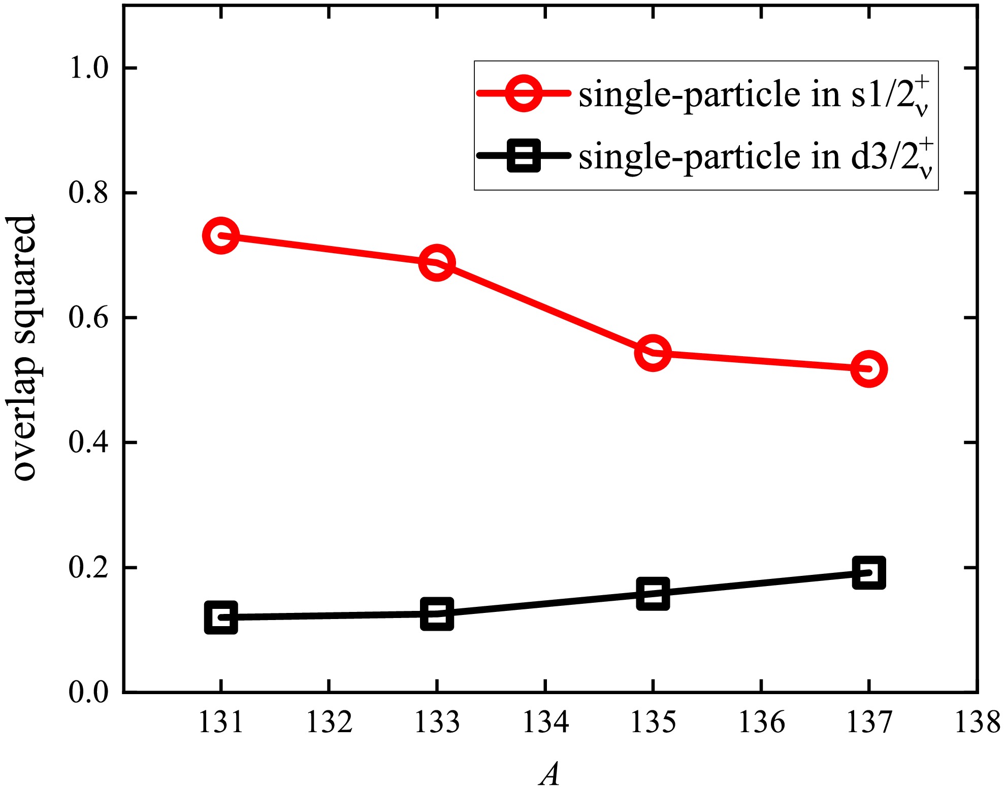
Figure 3. (color online) Overlap squared between the configurations
$ |J_{\pi}=0\rangle \otimes |S_{\nu}^{+}\otimes \nu s_{1/2}^{-1}\rangle$ (red circles) and$ |J_{\pi}=0 \rangle \otimes $ $ |D_{\nu}^{+}\otimes \nu d_{3/2}^{-1}\rangle$ (black squares) with the NPA wave function of the$1/2_{1}^{+}$ state versus the mass number A. -
According to the calculation using the Interacting Boson–Fermion model (IBFM), the
$ ^{131} {\rm{Te}}$ nucleus can be described as consisting of a$ ^{132} {\rm{Te}}$ core coupled with a neutron hole, and the configuration of the$ 1/2^{+}_{1} $ state is dominated by$ \nu s_{1/2}^{-1} $ with a small admixture of$ \nu d_{3/2}^{-1} $ [49]. References [50, 51] suggest that the$ 1/2^{+}_{1} $ state of$ ^{131} {\rm{Te}}$ is identified as a pure single-quasiparticle state. In our NPA calculation, the wave function of the$ 1/2_{1}^{+} $ state for$ ^{131} {\rm{Te}}$ is$ \left|1/2_{1}^+\right\rangle = 0.93|S_{\pi}^+ \rangle \otimes |S_{\nu}^+\otimes \nu s_{1/2}^{-1}\rangle -0.33|S_{\pi}^+ \rangle \otimes | D_{\nu}^+\otimes \nu d_{3/2}^{-1}\rangle+\cdots, $
(22) which agrees with Refs. [49−51].
Figure 3 presents the overlap squared between excitation configurations and the NPA wave function of the
$ 1/2_{1}^{+} $ state for$ ^{131} {\rm{Te}}$ ,$ ^{133} {\rm{Xe}}$ ,$ ^{135} {\rm{Ba}}$ , and$ ^{137} {\rm{Ce}}$ versus the mass number A. The red circles and black squares correspond to the$ |J_{\pi} = 0\rangle \otimes |S_{\nu}^{+}\otimes \nu s_{1/2}^{-1}\rangle $ and$ |J_{\pi} = 0 \rangle \otimes |D_{\nu}^{+}\otimes \nu d_{3/2}^{-1}\rangle $ configurations, respectively. We observe that the configuration$ |J_{\pi} = 0\rangle \otimes |S_{\nu}^{+}\otimes \nu s_{1/2}^{-1}\rangle $ dominates the$ 1/2_{1}^{+} $ state in these nuclei and decreases with increasing A, whereas the configuration$ |J_{\pi} = 0 \rangle \otimes |D_{\nu}^{+}\otimes \nu d_{3/2}^{-1}\rangle $ increases with A. This is consistent with the experimental energy levels of the$ 1/2_{1}^{+} $ state, which decrease with increasing A, because the single neutron hole energy of$ s_{1/2} $ is larger than that of$ d_{3/2} $ (see Table 1).
Figure 3. (color online) Overlap squared between the configurations
$ |J_{\pi}=0\rangle \otimes |S_{\nu}^{+}\otimes \nu s_{1/2}^{-1}\rangle$ (red circles) and$ |J_{\pi}=0 \rangle \otimes $ $ |D_{\nu}^{+}\otimes \nu d_{3/2}^{-1}\rangle$ (black squares) with the NPA wave function of the$1/2_{1}^{+}$ state versus the mass number A. -
Similar to the
$ 1/2^{+}_{1} $ state, the$ 5/2^{+}_{1} $ and$ 7/2^{+}_{1} $ states of$ ^{131} {\rm{Te}}$ are suggested to result essentially from the coupling of quasiparticles to the lowest-lying collective core states, and the configurations of these two states are dominated by$ \nu d_{3/2}^{-1} $ [49]. The wave functions of the$ 5/2_{1}^{+} $ and$ 7/2_{1}^{+} $ states for$ ^{131} {\rm{Te}}$ in our NPA calculations are$ \begin{split} & \left|5/2_{1}^+\right\rangle = 0.86|S_{\pi}^+\rangle\otimes|D_{\nu}^+\otimes \nu d_{3/2}^{-1}\rangle+\cdots, \\& \left|7/2_{1}^+\right\rangle = 0.73|S_{\pi}^+\rangle\otimes|D_{\nu}^+\otimes \nu d_{3/2}^{-1}\rangle+\cdots, \end{split} $

(23) respectively. Thus, the dominant components of both the
$ 5/2_{1}^{+} $ and$ 7/2_{1}^{+} $ states for$ ^{131} {\rm{Te}}$ are neutron excitations and is consistent with the IBFM results [49].The orbit with the lowest single-particle energy of valence protons is
$ g_{7/2} $ , and the$ h_{11/2} $ orbit has the lowest single-hole energy of valence neutron holes except for the$ d_{3/2} $ orbit, which cannot construct a neutron pair with high spin (see Table 1). The percentages of configurations$ \pi g_{7/2}^2 \otimes \nu h_{11/2}^{-2}d_{3/2}^{-1} $ and$ \pi g_{7/2}^2 \otimes \nu h_{11/2}^{-2}s_{1/2}^{-1} $ (the single neutron hole is considered to occupy the$ d_{3/2} $ or$ s_{1/2} $ orbit, which has relatively lower energy and positive parity) in wave functions of positive parity ($ 1/2^{+}_{1} \sim 23/2^{+}_{1} $ ) states for$ ^{131} {\rm{Te}}$ are calculated and presented in Fig. 4, denoted by solid black squares and red circles, respectively. The corresponding hollow symbols represent results given by the extended pairing plus multipole-multipole force model (EPQQM) [3] and are presented for comparison. The EPQQM is introduced in Ref. [52]. Our calculations show that the configuration$ \pi g_{7/2}^2 \otimes \nu h_{11/2}^{-2}d_{3/2}^{-1} $ dominates both the$ 5/2_{1}^{+} $ and$ 7/2_{1}^{+} $ states for$ ^{131} {\rm{Te}}$ , which is in agreement with the results from Ref. [3].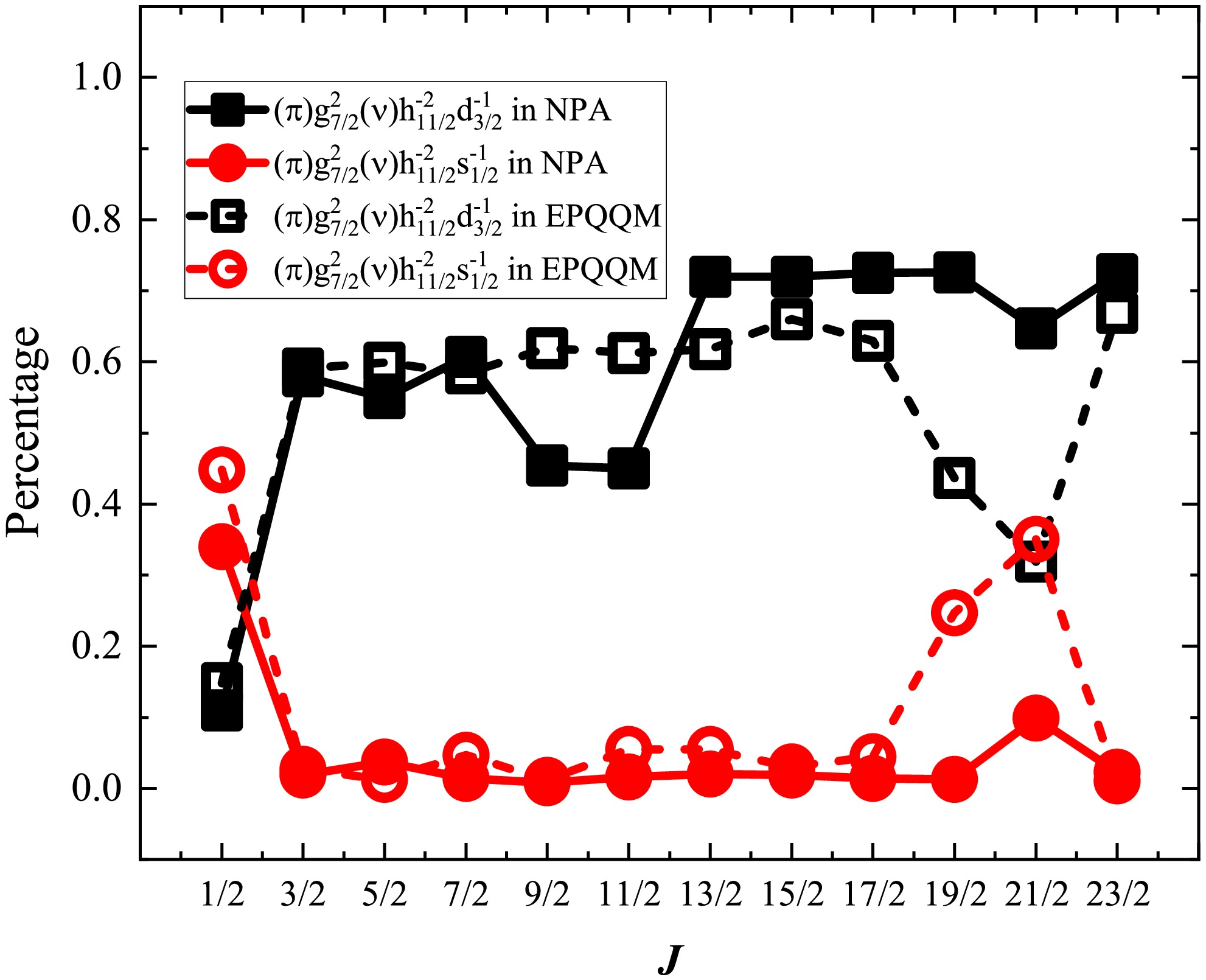
Figure 4. (color online) Percentages of configurations
$\pi g_{7/2}^2 \otimes \nu h_{11/2}^{-2}d_{3/2}^{-1}$ (solid black squares) and$\pi g_{7/2}^2 \otimes \nu h_{11/2}^{-2}s_{1/2}^{-1}$ (solid red circles) in the NPA wave functions of positive parity states for$^{131}{\rm{Te}}$ versus the angular momentum J. For comparison, the EPQQM results from Ref. [3] are also given, denoted by hollow symbols.In Fig. 5, the overlap squared between neutron excitation configurations and
$ |J_{\pi} = 2\rangle $ configurations with the wave functions of the$ 5/2_{1}^{+} $ and$ 7/2_{1}^{+} $ states is plotted versus the mass number A. The neutron excitation configurations of the$ 5/2_{1}^{+} $ and$ 7/2_{1}^{+} $ states (labeled by red circles and blue triangles) decrease rapidly at$ ^{133} {\rm{Xe}}$ , whereas$ |J_{\pi} = 2\rangle $ configurations (labeled by the black squares and green stars) increase with A. The$ 5/2_{1}^{+} $ and$ 7/2_{1}^{+} $ states of both$ ^{135} {\rm{Ba}}$ and$ ^{137} {\rm{Ce}}$ are dominated by$ |J_{\pi} = 2\rangle $ configurations. In addition, owing to the similarity in configurations of these two states for all four nuclei, the calculated$ B(E2) $ values of transitions$ 5/2_{1}^{+}\to3/2_{1}^{+} $ and$ 7/2_{1}^{+}\to3/2_{1}^{+} $ listed in Table 3 are very close.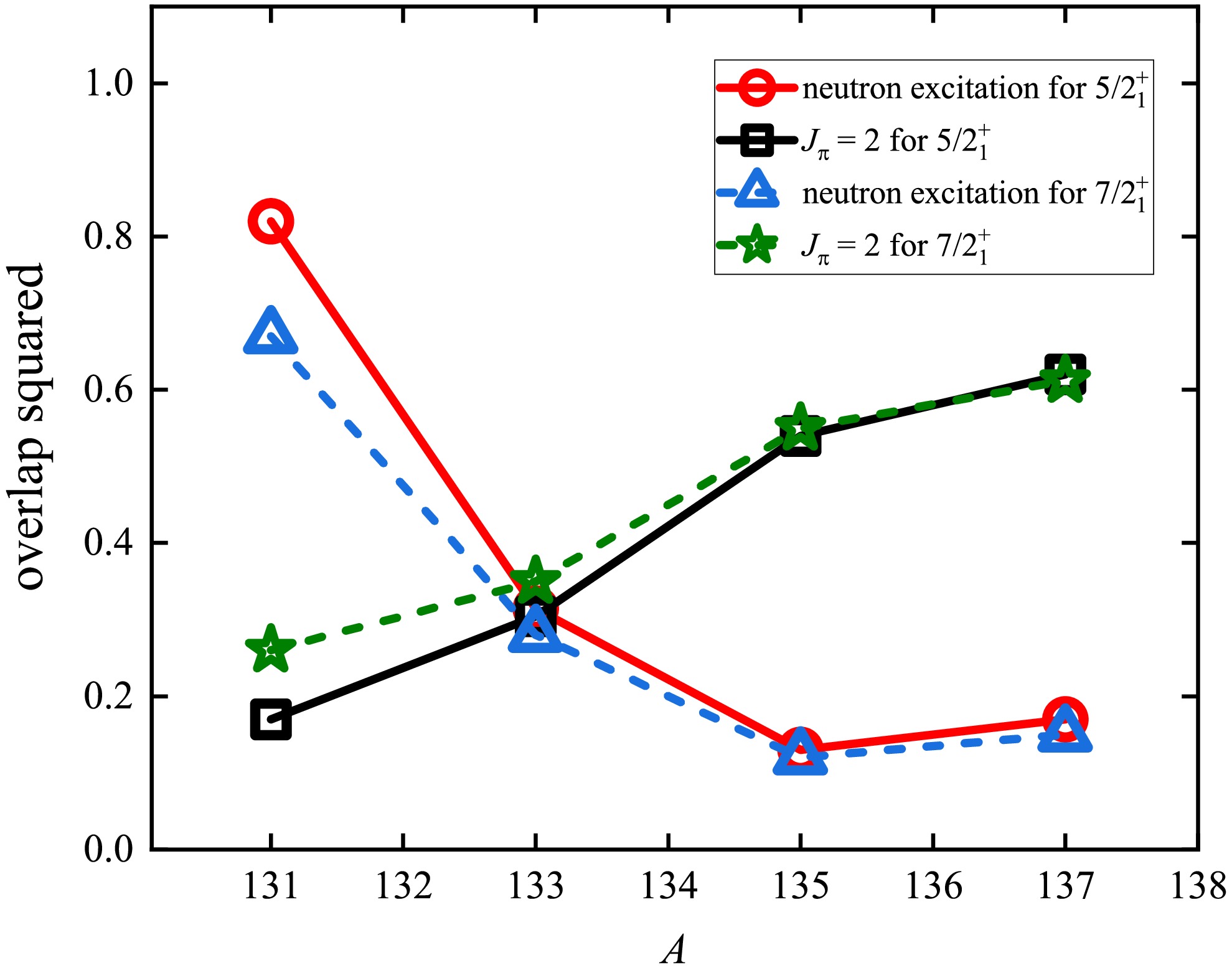
Figure 5. (color online) Overlap squared between the neutron excitation and
$|J_{\pi}=2\rangle$ configurations with the wave functions of the$5/2_{1}^{+}$ and$7/2_{1}^{+}$ states versus the mass number A. The red circles (blue triangles) represent neutron excitation configurations for the$5/2_{1}^{+}$ ($7/2_{1}^{+}$ ) states, whereas the black squares (green stars) represent$|J_{\pi}=2\rangle$ configurations for the$5/2_{1}^{+}$ ($7/2_{1}^{+}$ ) states. -
Similar to the
$ 1/2^{+}_{1} $ state, the$ 5/2^{+}_{1} $ and$ 7/2^{+}_{1} $ states of$ ^{131} {\rm{Te}}$ are suggested to result essentially from the coupling of quasiparticles to the lowest-lying collective core states, and the configurations of these two states are dominated by$ \nu d_{3/2}^{-1} $ [49]. The wave functions of the$ 5/2_{1}^{+} $ and$ 7/2_{1}^{+} $ states for$ ^{131} {\rm{Te}}$ in our NPA calculations are$ \begin{split} & \left|5/2_{1}^+\right\rangle = 0.86|S_{\pi}^+\rangle\otimes|D_{\nu}^+\otimes \nu d_{3/2}^{-1}\rangle+\cdots, \\& \left|7/2_{1}^+\right\rangle = 0.73|S_{\pi}^+\rangle\otimes|D_{\nu}^+\otimes \nu d_{3/2}^{-1}\rangle+\cdots, \end{split} $
(23) respectively. Thus, the dominant components of both the
$ 5/2_{1}^{+} $ and$ 7/2_{1}^{+} $ states for$ ^{131} {\rm{Te}}$ are neutron excitations and is consistent with the IBFM results [49].The orbit with the lowest single-particle energy of valence protons is
$ g_{7/2} $ , and the$ h_{11/2} $ orbit has the lowest single-hole energy of valence neutron holes except for the$ d_{3/2} $ orbit, which cannot construct a neutron pair with high spin (see Table 1). The percentages of configurations$ \pi g_{7/2}^2 \otimes \nu h_{11/2}^{-2}d_{3/2}^{-1} $ and$ \pi g_{7/2}^2 \otimes \nu h_{11/2}^{-2}s_{1/2}^{-1} $ (the single neutron hole is considered to occupy the$ d_{3/2} $ or$ s_{1/2} $ orbit, which has relatively lower energy and positive parity) in wave functions of positive parity ($ 1/2^{+}_{1} \sim 23/2^{+}_{1} $ ) states for$ ^{131} {\rm{Te}}$ are calculated and presented in Fig. 4, denoted by solid black squares and red circles, respectively. The corresponding hollow symbols represent results given by the extended pairing plus multipole-multipole force model (EPQQM) [3] and are presented for comparison. The EPQQM is introduced in Ref. [52]. Our calculations show that the configuration$ \pi g_{7/2}^2 \otimes \nu h_{11/2}^{-2}d_{3/2}^{-1} $ dominates both the$ 5/2_{1}^{+} $ and$ 7/2_{1}^{+} $ states for$ ^{131} {\rm{Te}}$ , which is in agreement with the results from Ref. [3].
Figure 4. (color online) Percentages of configurations
$\pi g_{7/2}^2 \otimes \nu h_{11/2}^{-2}d_{3/2}^{-1}$ (solid black squares) and$\pi g_{7/2}^2 \otimes \nu h_{11/2}^{-2}s_{1/2}^{-1}$ (solid red circles) in the NPA wave functions of positive parity states for$^{131}{\rm{Te}}$ versus the angular momentum J. For comparison, the EPQQM results from Ref. [3] are also given, denoted by hollow symbols.In Fig. 5, the overlap squared between neutron excitation configurations and
$ |J_{\pi} = 2\rangle $ configurations with the wave functions of the$ 5/2_{1}^{+} $ and$ 7/2_{1}^{+} $ states is plotted versus the mass number A. The neutron excitation configurations of the$ 5/2_{1}^{+} $ and$ 7/2_{1}^{+} $ states (labeled by red circles and blue triangles) decrease rapidly at$ ^{133} {\rm{Xe}}$ , whereas$ |J_{\pi} = 2\rangle $ configurations (labeled by the black squares and green stars) increase with A. The$ 5/2_{1}^{+} $ and$ 7/2_{1}^{+} $ states of both$ ^{135} {\rm{Ba}}$ and$ ^{137} {\rm{Ce}}$ are dominated by$ |J_{\pi} = 2\rangle $ configurations. In addition, owing to the similarity in configurations of these two states for all four nuclei, the calculated$ B(E2) $ values of transitions$ 5/2_{1}^{+}\to3/2_{1}^{+} $ and$ 7/2_{1}^{+}\to3/2_{1}^{+} $ listed in Table 3 are very close.
Figure 5. (color online) Overlap squared between the neutron excitation and
$|J_{\pi}=2\rangle$ configurations with the wave functions of the$5/2_{1}^{+}$ and$7/2_{1}^{+}$ states versus the mass number A. The red circles (blue triangles) represent neutron excitation configurations for the$5/2_{1}^{+}$ ($7/2_{1}^{+}$ ) states, whereas the black squares (green stars) represent$|J_{\pi}=2\rangle$ configurations for the$5/2_{1}^{+}$ ($7/2_{1}^{+}$ ) states. -
The
$ 23/2^{+}_{1} $ isomer of$ ^{131} {\rm{Te}}$ is proposed to have a three-quasineutron configuration obtained by coupling an$ h_{11/2} $ neutron hole to the$ 7^- $ core state [53]. According to the NSM calculations, the dominant configuration is 69%$ \pi g_{7/2}^2 \otimes \nu h_{11/2}^{-2}d_{3/2}^{-1} $ or 72%$ | J_{\pi} = 0 \rangle \otimes | J_{\nu} = 23/2 \rangle $ of the$ 23/2^{+}_{1} $ state for$ ^{131} {\rm{Te}}$ , and it is 56%$ | J_{\pi} = 0 \rangle \otimes | J_{\nu} = 23/2 \rangle $ with 29%$ | J_{\pi} = 2 \rangle \otimes | J_{\nu} = 23/2 \rangle $ mixing for$ ^{133} {\rm{Xe}}$ [54]. Reference [11] also indicates that the$ 23/2^{+}_{1} $ states contain 81%, 60%, and 44%$ \nu h_{11/2}^{-2}d_{3/2}^{-1} $ configurations or 72%, 54%, and 43%$ | J_{\pi} = 0 \rangle \otimes | J_{\nu} = 23/2 \rangle $ configurations for$ ^{131} {\rm{Te}}$ ,$ ^{133} {\rm{Xe}}$ , and$ ^{135} {\rm{Ba}}$ , respectively.The wave function of the
$ 23/2_{1}^{+} $ state for$ ^{131} {\rm{Te}}$ calculated using the NPA is$ \begin{split} \left|23/2_{1}^+\right\rangle = &|S_{\pi}^+\rangle \otimes [ 0.93|{\cal{J}}_{\nu}^-\otimes \nu h_{11/2}^{-1}\rangle -0.92|I_{\nu}^-\otimes \nu h_{11/2}^{-1}\rangle \\& -0.92|{\cal{A}}_{\nu}^{(10)}\otimes \nu d_{3/2}^{-1}\rangle ] +\cdots, \end{split}$

(24) which is dominated by the neutron excitation configuration. Because neutron collective pairs with negative parity are primarily composed of
$ \nu h_{11/2}^{-1}d_{3/2}^{-1} $ , the$ \nu h_{11/2}^{-2}d_{3/2}^{-1} $ configuration plays an important role in the$ 23/2_{1}^{+} $ state, as presented in Fig. 4, which agrees closely with Refs. [3, 11, 53, 54].The overlap squared between configurations
$ |J_{\pi} = 0\rangle $ and$ |J_{\pi} = 2\rangle $ with the wave functions of the$ 23/2_{1}^{+} $ state versus the mass number A is plotted in Fig. 6, denoted by red circles and black squares, respectively. The$ |J_{\pi} = 0\rangle $ ($ |J_{\pi} = 2\rangle $ ) configuration decreases (increases) with A. The NPA calculations provide 87%, 67%, and 54%$ |J_{\pi} = 0\rangle \otimes | J_{\nu} = 23/2 \rangle $ configurations for$ ^{131} {\rm{Te}}$ ,$ ^{133} {\rm{Xe}}$ , and$ ^{135} {\rm{Ba}}$ , respectively, which are close to the results in Refs. [11, 54].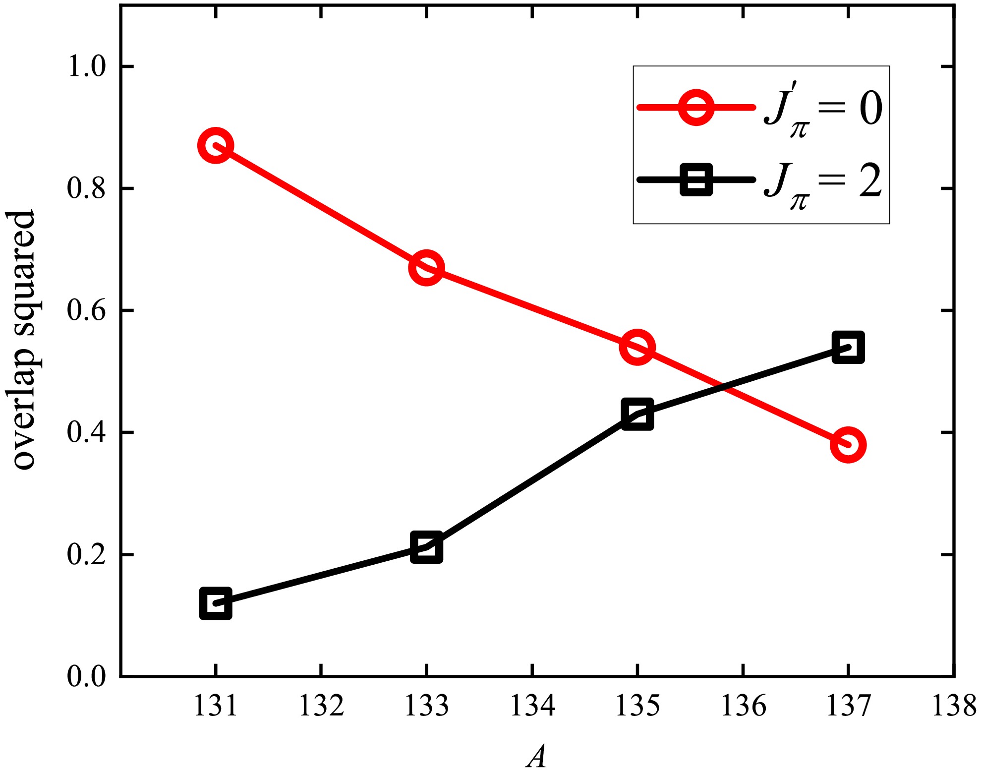
Figure 6. (color online) Overlap squared between the configurations
$|J_{\pi}=0\rangle$ (red circles) and$|J_{\pi}=2\rangle$ (black squares) with the wave functions of the$23/2_{1}^{+}$ state versus the mass number A. -
The
$ 23/2^{+}_{1} $ isomer of$ ^{131} {\rm{Te}}$ is proposed to have a three-quasineutron configuration obtained by coupling an$ h_{11/2} $ neutron hole to the$ 7^- $ core state [53]. According to the NSM calculations, the dominant configuration is 69%$ \pi g_{7/2}^2 \otimes \nu h_{11/2}^{-2}d_{3/2}^{-1} $ or 72%$ | J_{\pi} = 0 \rangle \otimes | J_{\nu} = 23/2 \rangle $ of the$ 23/2^{+}_{1} $ state for$ ^{131} {\rm{Te}}$ , and it is 56%$ | J_{\pi} = 0 \rangle \otimes | J_{\nu} = 23/2 \rangle $ with 29%$ | J_{\pi} = 2 \rangle \otimes | J_{\nu} = 23/2 \rangle $ mixing for$ ^{133} {\rm{Xe}}$ [54]. Reference [11] also indicates that the$ 23/2^{+}_{1} $ states contain 81%, 60%, and 44%$ \nu h_{11/2}^{-2}d_{3/2}^{-1} $ configurations or 72%, 54%, and 43%$ | J_{\pi} = 0 \rangle \otimes | J_{\nu} = 23/2 \rangle $ configurations for$ ^{131} {\rm{Te}}$ ,$ ^{133} {\rm{Xe}}$ , and$ ^{135} {\rm{Ba}}$ , respectively.The wave function of the
$ 23/2_{1}^{+} $ state for$ ^{131} {\rm{Te}}$ calculated using the NPA is$ \begin{split} \left|23/2_{1}^+\right\rangle = &|S_{\pi}^+\rangle \otimes [ 0.93|{\cal{J}}_{\nu}^-\otimes \nu h_{11/2}^{-1}\rangle -0.92|I_{\nu}^-\otimes \nu h_{11/2}^{-1}\rangle \\& -0.92|{\cal{A}}_{\nu}^{(10)}\otimes \nu d_{3/2}^{-1}\rangle ] +\cdots, \end{split}$
(24) which is dominated by the neutron excitation configuration. Because neutron collective pairs with negative parity are primarily composed of
$ \nu h_{11/2}^{-1}d_{3/2}^{-1} $ , the$ \nu h_{11/2}^{-2}d_{3/2}^{-1} $ configuration plays an important role in the$ 23/2_{1}^{+} $ state, as presented in Fig. 4, which agrees closely with Refs. [3, 11, 53, 54].The overlap squared between configurations
$ |J_{\pi} = 0\rangle $ and$ |J_{\pi} = 2\rangle $ with the wave functions of the$ 23/2_{1}^{+} $ state versus the mass number A is plotted in Fig. 6, denoted by red circles and black squares, respectively. The$ |J_{\pi} = 0\rangle $ ($ |J_{\pi} = 2\rangle $ ) configuration decreases (increases) with A. The NPA calculations provide 87%, 67%, and 54%$ |J_{\pi} = 0\rangle \otimes | J_{\nu} = 23/2 \rangle $ configurations for$ ^{131} {\rm{Te}}$ ,$ ^{133} {\rm{Xe}}$ , and$ ^{135} {\rm{Ba}}$ , respectively, which are close to the results in Refs. [11, 54].
Figure 6. (color online) Overlap squared between the configurations
$|J_{\pi}=0\rangle$ (red circles) and$|J_{\pi}=2\rangle$ (black squares) with the wave functions of the$23/2_{1}^{+}$ state versus the mass number A. -
For the
$ 11/2^{-}_{1} $ and$ 15/2^{-}_{1} $ states ($ 21/2^{-}_{1} $ and$ 23/2^{-}_{1} $ states) of$ ^{131} {\rm{Te}}$ and$ ^{133} {\rm{Xe}}$ , the NSM calculations indicate that the dominant proton configurations are$ |J_{\pi} = 0\rangle $ ($ |J_{\pi} = 6\rangle $ ), whereas for the$ 19/2^{-}_{1} $ states, the dominant configurations are$ |J_{\pi} = 4\rangle $ and$ |J_{\pi} = 6\rangle $ [11, 54]. For$ ^{137} {\rm{Ce}}$ , Ref. [55] suggests that the$ 11/2^{-}_{1} $ isomeric state is based on the$ h_{11/2} $ neutron hole coupled to the even–even nuclear core, and the$ 15/2^{-}_{1} $ ($ 19/2^{-}_{1} $ ) state may be assigned the$ \nu h_{11/2}^{-1} \otimes 2^+ $ ($ \nu h_{11/2}^{-1} \otimes 4^+ $ ) multiplet.The wave functions of the
$ 11/2^{-}_{1} $ state for$ ^{131} {\rm{Te}}$ ,$ ^{133} {\rm{Xe}}$ ,$ ^{135} {\rm{Ba}}$ , and$ ^{137} {\rm{Ce}}$ in this paper are$ \begin{split} & \left|11/2_{1}^-\right\rangle = 0.93|S_{\pi}^+\rangle\otimes|S_{\nu}^+\otimes \nu h_{11/2}^{-1}\rangle+\cdots, \\& \left|11/2_{1}^-\right\rangle = 0.98|(S_{\pi}^+)^{N_{\pi}/2}\rangle\otimes|S_{\nu}^+\otimes \nu h_{11/2}^{-1}\rangle+\cdots, \\& \left|11/2_{1}^-\right\rangle = 0.84|(S_{\pi}^+)^{N_{\pi}/2}\rangle\otimes|S_{\nu}^+\otimes \nu h_{11/2}^{-1}\rangle+\cdots, \\& \left|11/2_{1}^-\right\rangle = 0.93|(S_{\pi}^+)^{N_{\pi}/2}\rangle\otimes|S_{\nu}^+\otimes \nu h_{11/2}^{-1}\rangle+\cdots, \end{split} $

(25) respectively, which are all dominated by the neutron excitation configuration. The dominant components of
$ |S_{\nu}^{+} \otimes \nu h_{11/2}^{-1}\rangle $ configuration are$ \nu h^{-3}_{11/2} $ and$ \nu h^{-1}_{11/2}d^{-2}_{3/2} $ ; thus, the NPA calculations assign the$ \nu h^{-3}_{11/2} $ configuration percentages as 55%, 53%, 41%, and 30%, and the$ \nu h^{-1}_{11/2}d^{-2}_{3/2} $ configuration percentages as 38%, 36%, 48%, and 61% of the$ 11/2^{-}_{1} $ state for$ ^{131} {\rm{Te}}$ ,$ ^{133} {\rm{Xe}}$ ,$ ^{135} {\rm{Ba}}$ , and$ ^{137} {\rm{Ce}}$ , respectively.In our NPA calculations, the wave functions of
$ 13/2_{1}^{-} \sim 23/2_{1}^{-} $ and$ 27/2_{1}^{-} $ states for$ ^{131} {\rm{Te}}$ are$\begin{split} |13/2_{1}^-\rangle= & 0.74|S_{\pi}^+\rangle\otimes|D_{\nu}^+\otimes \nu h_{11/2}^{-1}\rangle \\& +0.52|D_{\pi}^+\rangle\otimes|S_{\nu}^+\otimes \nu h_{11/2}^{-1}\rangle+\cdots, \\ |15/2_{1}^-\rangle = & 0.82|S_{\pi}^+\rangle\otimes|D_{\nu}^+\otimes \nu h_{11/2}^{-1}\rangle \\& +0.59|S_{\pi}^+\rangle\otimes|I_{\nu}^-\otimes \nu d_{3/2}^{-1}\rangle+\cdots, \\ |17/2_{1}^-\rangle = & -0.91|G_{\pi}^+\rangle\otimes|S_{\nu}^+\otimes \nu h_{11/2}^{-1}\rangle \\& +0.57|G_{\pi}^+\rangle\otimes|{\cal{A}}_{\nu}^{(6)}\otimes \nu h_{11/2}^{-1}\rangle+\cdots, \\ |19/2_{1}^-\rangle = & -0.88|G_{\pi}^+\rangle\otimes|S_{\nu}^+\otimes \nu h_{11/2}^{-1}\rangle \\& +0.58|G_{\pi}^+\rangle\otimes|{\cal{A}}_{\nu}^{(6)}\otimes \nu h_{11/2}^{-1}\rangle+\cdots, \\ |21/2_{1}^-\rangle = & 0.79|I_{\pi}^+\rangle\otimes|S_{\nu}^+\otimes \nu h_{11/2}^{-1}\rangle +0.51|G_{\pi}^+\rangle\otimes|D_{\nu}^+\otimes \nu h_{11/2}^{-1}\rangle \\& -0.50|I_{\pi}^+\rangle\otimes|{\cal{A}}_{\nu}^{(6)}\otimes \nu h_{11/2}^{-1}\rangle+\cdots, \\ |23/2_{1}^-\rangle = & -0.73|I_{\pi}^+\rangle\otimes|S_{\nu}^+\otimes \nu h_{11/2}^{-1}\rangle -0.61|G_{\pi}^+\rangle\otimes|D_{\nu}^+\otimes \nu h_{11/2}^{-1}\rangle \\& +0.49|I_{\pi}^+\rangle\otimes|{\cal{A}}_{\nu}^{(6)}\otimes \nu h_{11/2}^{-1}\rangle+\cdots, \\ |27/2_{1}^-\rangle = & 0.96|S_{\pi}^+\rangle\otimes|{\cal{A}}_{\nu}^{(10)}\otimes \nu h_{11/2}^{-1}\rangle \\& -0.96|S_{\pi}^+\rangle\otimes|{\cal{A}}_{\nu}^{(8)}\otimes \nu h_{11/2}^{-1}\rangle+\cdots,\\[-1pt] \end{split} $

(26) respectively, and
$ 13/2_{1}^{-} $ ,$ 15/2_{1}^{-} $ , and$ 27/2_{1}^{-} $ states are dominated by the neutron excitation. In addition, all these states exhibit a significant component of$ \nu h_{11/2}^{-1} $ .The overlap squared between the neutron excitation and
$ |J_{\pi} = 2\rangle $ configurations with the wave functions of the$ 13/2_{1}^{-} $ and$ 15/2_{1}^{-} $ states are plotted in Fig. 7 versus the mass number A. The red circles (blue triangles) and black squares (green stars) correspond to the neutron excitation configuration and$ |J_{\pi} = 2\rangle $ components for the$ 13/2_{1}^{-} $ ($ 15/2_{1}^{-} $ ) state, respectively. Both the$ 13/2_{1}^{-} $ and$ 15/2_{1}^{-} $ states of$ ^{131} {\rm{Te}}$ are dominated by the neutron excitations, whereas those for$ ^{135} {\rm{Ba}}$ and$ ^{137} {\rm{Ce}}$ are dominated by the configuration$ |J_{\pi} = 2\rangle $ .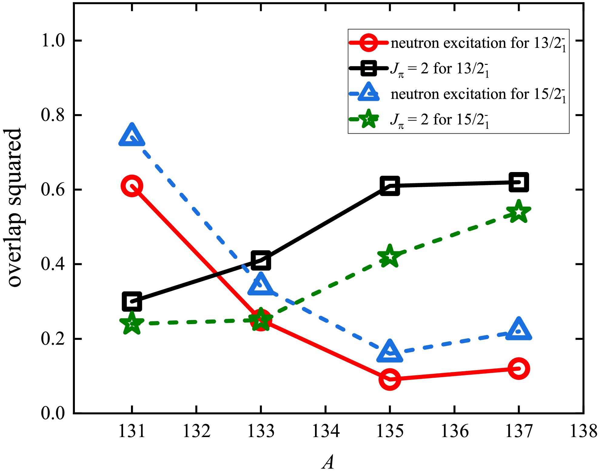
Figure 7. (color online) Overlap squared between the neutron excitation and
$|J_{\pi}=2\rangle$ configurations with the wave functions of the$13/2_{1}^{-}$ and$15/2_{1}^{-}$ states versus the mass number A. The red circles and black squares correspond to the neutron excitation configuration and$|J_{\pi}=2\rangle$ components for the$13/2_{1}^{-}$ state, respectively. The blue triangles and green stars correspond to the neutron excitation configuration and$|J_{\pi}=2\rangle$ components for the$15/2_{1}^{-}$ state, respectively.Similar overlap squared between configurations
$ |J_{\pi} = 4\rangle $ and$ |J_{\pi} = 2\rangle $ with the wave functions of the$ 17/2_{1}^{-} $ and$ 19/2_{1}^{-} $ states are presented in Fig. 8, and those between configurations$ |J_{\pi} = 6\rangle $ and the wave functions of the$ 21/2_{1}^{-} $ and$ 23/2_{1}^{-} $ states are presented in Fig. 9. The dominant component is$ |J_{\pi} = 4\rangle $ for$ 17/2_{1}^{-} $ and$ 19/2_{1}^{-} $ states of$ ^{131} {\rm{Te}}$ and$ ^{133} {\rm{Xe}}$ ,$ |J_{\pi} = 2\rangle $ for$ 17/2_{1}^{-} $ states of$ ^{135} {\rm{Ba}}$ and$ ^{137} {\rm{Ce}}$ , and$ |J_{\pi} = 6\rangle $ of$ 21/2_{1}^{-} $ and$ 23/2_{1}^{-} $ states of$ ^{131} {\rm{Te}}$ ,$ ^{133} {\rm{Xe}}$ ,$ ^{135} {\rm{Ba}}$ , and$ ^{137} {\rm{Ce}}$ .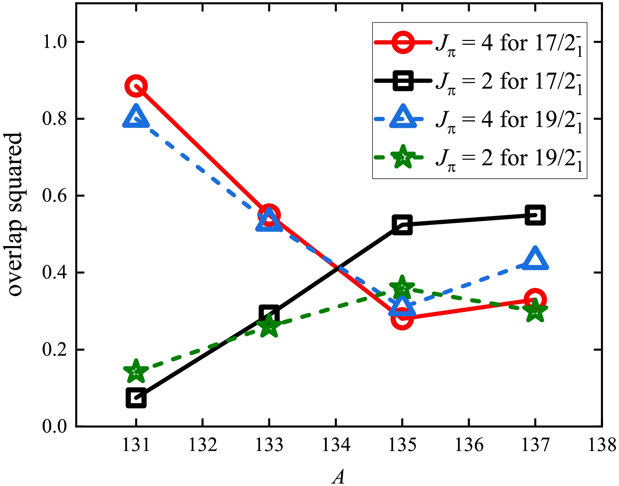
Figure 8. (color online) Overlap squared between configurations
$|J_{\pi}=4\rangle$ and$|J_{\pi}=2\rangle$ with the wave functions of the$17/2_{1}^{-}$ and$19/2_{1}^{-}$ states versus the mass number A. The red circles and black squares correspond to configurations$|J_{\pi}=4\rangle$ and$|J_{\pi}=2\rangle$ for the$17/2_{1}^{-}$ state. The blue triangles and green stars correspond to configurations$|J_{\pi}=4\rangle$ and$|J_{\pi}=2\rangle$ for the$19/2_{1}^{-}$ state.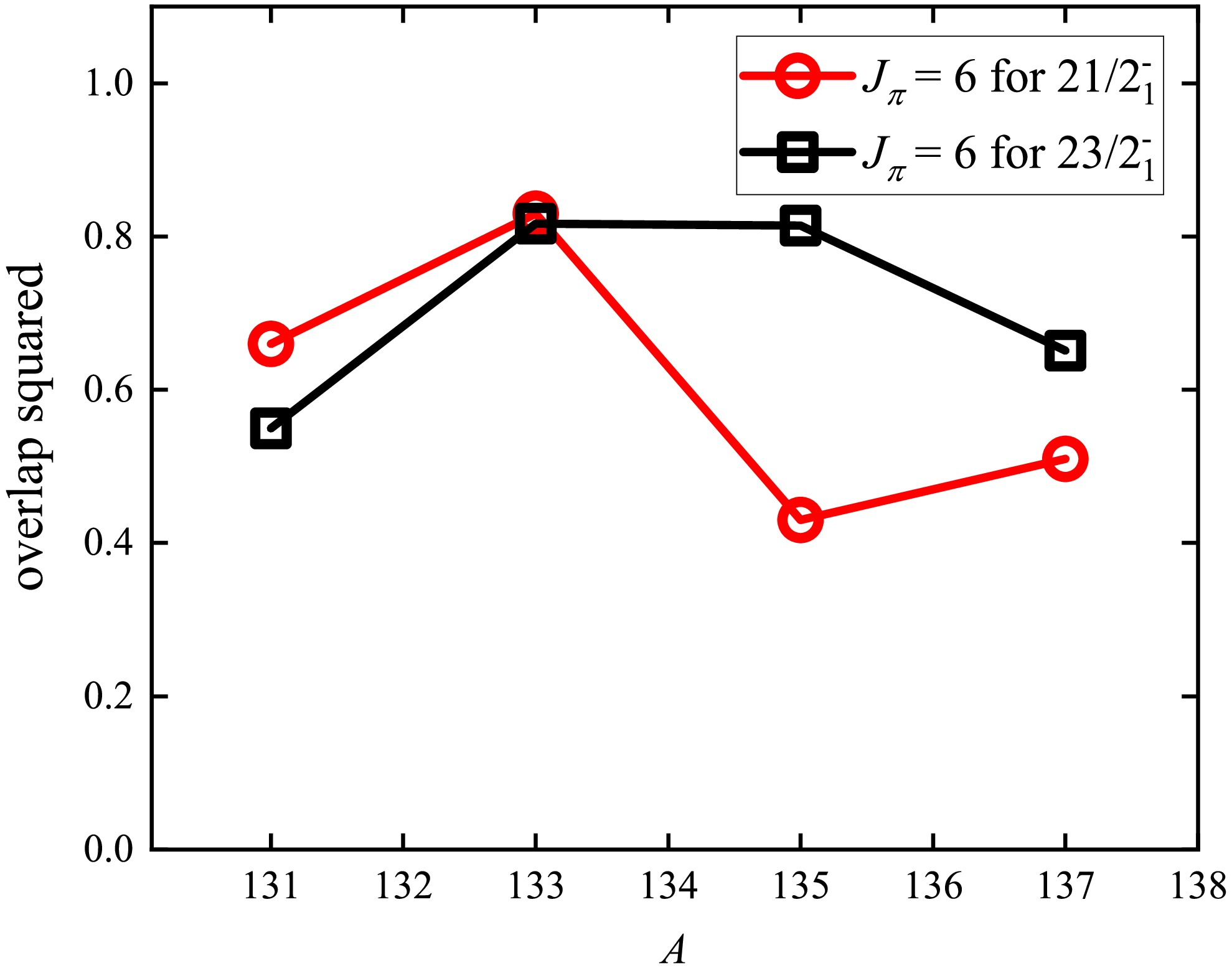
Figure 9. (color online) Overlap squared between configurations
$|J_{\pi}=6\rangle$ and the wave functions of the$21/2_{1}^{-}$ and$23/2_{1}^{-}$ states versus the mass number A. The red circles and black squares correspond to configurations$|J_{\pi}=6\rangle$ for the$21/2_{1}^{-}$ and$23/2_{1}^{-}$ states, respectively.Energies of the Hamiltonian
$ H_P $ and$ H_Q $ in single-j shells for an odd system with only one pair can be analytically obtained using the simplified Eqs. (30), (33), and (34) given in Appendix A. Thus, similar to Ref. [27], the configuration pictures of the$ 17/2_{1}^{-} $ ,$ 19/2_{1}^{-} $ ,$ 21/2_{1}^{-} $ , and$ 23/2_{1}^{-} $ states for$ ^{131} {\rm{Te}}$ can be understood from a simple perspective of single-j shells (protons in the$ g_{7/2} $ orbit and neutron holes in the$ h_{11/2} $ orbit). For valence protons, we consider the$ S^{+}_{\pi} $ and$ G^{+}_{\pi} $ ($ I^{+}_{\pi} $ ) pairs in the$ 17/2_{1}^{-} $ and$ 19/2_{1}^{-} $ ($ 21/2_{1}^{-} $ and$ 23/2_{1}^{-} $ ) states, whereas for valence neutron holes, we consider$ S_{\nu}^{+}\otimes \nu h_{11/2}^{-1} $ for all these four states, as well as$ {\cal{A}}_{\nu}^{(4)}\otimes \nu h_{11/2}^{-1} $ ($ {\cal{A}}_{\nu}^{(6)}\otimes \nu h_{11/2}^{-1} $ ) in the$ 17/2_{1}^{-} $ and$ 19/2_{1}^{-} $ ($ 21/2_{1}^{-} $ and$ 23/2_{1}^{-} $ ) states. The matrix elements of$ H_P $ and$ H_Q $ in single-j shells (and$ H_0 $ in many-j shells) are presented in Table 5.$^{131}{\rm{Te}}$ 

$H_{0}$ 

$-V_{0}$ 

$-V_{2}$ 

$-V_{4}$ 

$-V_{Q}$ 

$S_{\nu}^{+}\otimes \nu h_{11/2}^{-1}$ 

$0.422$ 

$\dfrac{553}{500}$ 

0 0 $\dfrac{677}{313\pi}$ 

$({\cal{A}}_{\nu}^{(4)}\otimes \nu h_{11/2}^{-1})_{J_{\nu} = 17/2}$ 

$0.109$ 

0 $<0.001$ 

$\dfrac{388}{785\pi}$ 

$\dfrac{1629}{1010\pi}$ 

$({\cal{A}}_{\nu}^{(4)}\otimes \nu h_{11/2}^{-1})_{J_{\nu} = 19/2}$ 

$0.089$ 

0 $<0.001$ 

$\dfrac{1038}{3079\pi}$ 

$\dfrac{801}{637\pi}$ 

$({\cal{A}}_{\nu}^{(6)}\otimes \nu h_{11/2}^{-1})_{J_{\nu} = 21/2}$ 

$0.170$ 

0 $<0.001$ 

$<0.001$ 

$\dfrac{2540}{1953\pi}$ 

$({\cal{A}}_{\nu}^{(6)}\otimes \nu h_{11/2}^{-1})_{J_{\nu} = 23/2}$ 

$0.097$ 

0 $<0.001$ 

$<0.001$ 

$\dfrac{989}{1070\pi}$ 

$S_{\pi}^{+}$ 

$0.925$ 

$\dfrac{21}{28}$ 

0 0 $\dfrac{121}{56\pi}$ 

$G_{\pi}^{+}$ 

$0.199$ 

0 0 $\dfrac{667}{1175\pi}$ 

$\dfrac{121}{168\pi}$ 

$I_{\pi}^{+}$ 

$0.003$ 

0 0 0 $\dfrac{121}{168\pi}$ 

Table 5. Matrix elements (in MeV) of
$H_{0}$ ,$V_{0}$ ,$V_{2}$ ,$V_{4}$ , and$V_{Q}$ for a few configurations of$^{131}{\rm{Te}}$ with the phenomenological NSM Hamiltonian. The matrix elements of single-particle energies$H_{0}$ are calculated in many-j shells. The results of$V_{0}$ ,$V_{2}$ ,$V_{4}$ , and$V_{Q}$ are for single-j shells with valence protons in the$g_{7/2}$ orbit and valence neutron holes in the$h_{11/2}$ orbit; these matrix elements are derived analytically using Eqs. (30), (33), and (34) in Appendix A. Both$V_{10}$ and$V_{Q_{\pi\nu}}$ equal zero in these configurations with such single-j shells and are not listed here.According to Table 5, we have
$ \begin{array}{r}\\ \langle G_{\pi}^+\otimes S_{\nu}^+\otimes \nu h_{11/2}^{-1}|H|G_{\pi}^+\otimes S_{\nu}^+\otimes \nu h_{11/2}^{-1}\rangle \approx -1.583\; {\rm{MeV}}, \\ \langle S_{\pi}^+ \otimes ({\cal{A}}^{(4)}_{\nu} \otimes \nu h_{11/2}^{-1})_{J_{\nu} = 17/2} | H | S_{\pi}^+ \otimes ({\cal{A}}^{(4)}_{\nu} \otimes \nu h_{11/2}^{-1})_{J_{\nu} = 17/2}\rangle \approx -1.074 \; {\rm{MeV}}, \\ \langle S_{\pi}^+\otimes ({\cal{A}}^{(4)}_{\nu} \otimes \nu h_{11/2}^{-1})_{J_{\nu} = 19/2} |H|S_{\pi}^+\otimes ({\cal{A}}^{(4)}_{\nu} \otimes \nu h_{11/2}^{-1})_{J_{\nu} = 19/2} \rangle \approx -0.931 \; {\rm{MeV}} \end{array} $

(27) for the
$ 17/2_{1}^{-} $ and$ 19/2_{1}^{-} $ states, and$ \begin{array}{r} \langle I_{\pi}^+\otimes S_{\nu}^+\otimes \nu h_{11/2}^{-1}|H|I_{\pi}^+\otimes S_{\nu}^+\otimes \nu h_{11/2}^{-1}\rangle \approx -1.599 \; {\rm{MeV}}, \\ \langle S_{\pi}^+\otimes ({\cal{A}}^{(6)}_{\nu} \otimes \nu h_{11/2}^{-1})_{J_{\nu} = 21/2} |H|S_{\pi}^+\otimes ({\cal{A}}^{(6)}_{\nu} \otimes \nu h_{11/2}^{-1})_{J_{\nu} = 21/2} \rangle \approx -0.757 \; {\rm{MeV}}, \\ \langle S_{\pi}^+\otimes ({\cal{A}}^{(6)}_{\nu} \otimes \nu h_{11/2}^{-1})_{J_{\nu} = 23/2} |H|S_{\pi}^+\otimes ({\cal{A}}^{(6)}_{\nu} \otimes \nu h_{11/2}^{-1})_{J_{\nu} = 23/2} \rangle \approx -0.710 \; {\rm{MeV}} \end{array} $

(28) for the
$ 21/2_{1}^{-} $ and$ 23/2_{1}^{-} $ states. The energies of neutron excitation configurations are much larger than those of$ G_{\pi}^{+}\otimes S_{\nu}^{+}\otimes \nu h_{11/2}^{-1} $ and$ I_{\pi}^{+}\otimes S_{\nu}^{+}\otimes \nu h_{11/2}^{-1} $ . Thus, the$ 17/2_{1}^{-} $ and$ 19/2_{1}^{-} $ ($ 21/2_{1}^{-} $ and$ 23/2_{1}^{-} $ ) states of$ ^{131} {\rm{Te}}$ are dominated by configuration$ G_{\pi}^{+}\otimes S_{\nu}^{+}\otimes \nu h_{11/2}^{-1} $ ($ I_{\pi}^{+}\otimes S_{\nu}^{+}\otimes \nu h_{11/2}^{-1} $ ), which is consistent with Eq. (26). This indicates that the$ 17/2_{1}^{-} $ and$ 19/2_{1}^{-} $ ($ 21/2_{1}^{-} $ and$ 23/2_{1}^{-} $ ) states of$ ^{131} {\rm{Te}}$ can be described as consisting of the$ 4^+_1 $ ($ 6^+_1 $ ) states of$ ^{132} {\rm{Te}}$ , which is suggested to be dominated by proton excitations$ G_{\pi}^{+}\otimes S_{\nu}^{+} $ ($ I_{\pi}^{+}\otimes S_{\nu}^{+} $ ) in Ref. [27], coupled with a neutron hole occupies the$ h_{11/2} $ orbit. -
For the
$ 11/2^{-}_{1} $ and$ 15/2^{-}_{1} $ states ($ 21/2^{-}_{1} $ and$ 23/2^{-}_{1} $ states) of$ ^{131} {\rm{Te}}$ and$ ^{133} {\rm{Xe}}$ , the NSM calculations indicate that the dominant proton configurations are$ |J_{\pi} = 0\rangle $ ($ |J_{\pi} = 6\rangle $ ), whereas for the$ 19/2^{-}_{1} $ states, the dominant configurations are$ |J_{\pi} = 4\rangle $ and$ |J_{\pi} = 6\rangle $ [11, 54]. For$ ^{137} {\rm{Ce}}$ , Ref. [55] suggests that the$ 11/2^{-}_{1} $ isomeric state is based on the$ h_{11/2} $ neutron hole coupled to the even–even nuclear core, and the$ 15/2^{-}_{1} $ ($ 19/2^{-}_{1} $ ) state may be assigned the$ \nu h_{11/2}^{-1} \otimes 2^+ $ ($ \nu h_{11/2}^{-1} \otimes 4^+ $ ) multiplet.The wave functions of the
$ 11/2^{-}_{1} $ state for$ ^{131} {\rm{Te}}$ ,$ ^{133} {\rm{Xe}}$ ,$ ^{135} {\rm{Ba}}$ , and$ ^{137} {\rm{Ce}}$ in this paper are$ \begin{split} & \left|11/2_{1}^-\right\rangle = 0.93|S_{\pi}^+\rangle\otimes|S_{\nu}^+\otimes \nu h_{11/2}^{-1}\rangle+\cdots, \\& \left|11/2_{1}^-\right\rangle = 0.98|(S_{\pi}^+)^{N_{\pi}/2}\rangle\otimes|S_{\nu}^+\otimes \nu h_{11/2}^{-1}\rangle+\cdots, \\& \left|11/2_{1}^-\right\rangle = 0.84|(S_{\pi}^+)^{N_{\pi}/2}\rangle\otimes|S_{\nu}^+\otimes \nu h_{11/2}^{-1}\rangle+\cdots, \\& \left|11/2_{1}^-\right\rangle = 0.93|(S_{\pi}^+)^{N_{\pi}/2}\rangle\otimes|S_{\nu}^+\otimes \nu h_{11/2}^{-1}\rangle+\cdots, \end{split} $
(25) respectively, which are all dominated by the neutron excitation configuration. The dominant components of
$ |S_{\nu}^{+} \otimes \nu h_{11/2}^{-1}\rangle $ configuration are$ \nu h^{-3}_{11/2} $ and$ \nu h^{-1}_{11/2}d^{-2}_{3/2} $ ; thus, the NPA calculations assign the$ \nu h^{-3}_{11/2} $ configuration percentages as 55%, 53%, 41%, and 30%, and the$ \nu h^{-1}_{11/2}d^{-2}_{3/2} $ configuration percentages as 38%, 36%, 48%, and 61% of the$ 11/2^{-}_{1} $ state for$ ^{131} {\rm{Te}}$ ,$ ^{133} {\rm{Xe}}$ ,$ ^{135} {\rm{Ba}}$ , and$ ^{137} {\rm{Ce}}$ , respectively.In our NPA calculations, the wave functions of
$ 13/2_{1}^{-} \sim 23/2_{1}^{-} $ and$ 27/2_{1}^{-} $ states for$ ^{131} {\rm{Te}}$ are$\begin{split} |13/2_{1}^-\rangle= & 0.74|S_{\pi}^+\rangle\otimes|D_{\nu}^+\otimes \nu h_{11/2}^{-1}\rangle \\& +0.52|D_{\pi}^+\rangle\otimes|S_{\nu}^+\otimes \nu h_{11/2}^{-1}\rangle+\cdots, \\ |15/2_{1}^-\rangle = & 0.82|S_{\pi}^+\rangle\otimes|D_{\nu}^+\otimes \nu h_{11/2}^{-1}\rangle \\& +0.59|S_{\pi}^+\rangle\otimes|I_{\nu}^-\otimes \nu d_{3/2}^{-1}\rangle+\cdots, \\ |17/2_{1}^-\rangle = & -0.91|G_{\pi}^+\rangle\otimes|S_{\nu}^+\otimes \nu h_{11/2}^{-1}\rangle \\& +0.57|G_{\pi}^+\rangle\otimes|{\cal{A}}_{\nu}^{(6)}\otimes \nu h_{11/2}^{-1}\rangle+\cdots, \\ |19/2_{1}^-\rangle = & -0.88|G_{\pi}^+\rangle\otimes|S_{\nu}^+\otimes \nu h_{11/2}^{-1}\rangle \\& +0.58|G_{\pi}^+\rangle\otimes|{\cal{A}}_{\nu}^{(6)}\otimes \nu h_{11/2}^{-1}\rangle+\cdots, \\ |21/2_{1}^-\rangle = & 0.79|I_{\pi}^+\rangle\otimes|S_{\nu}^+\otimes \nu h_{11/2}^{-1}\rangle +0.51|G_{\pi}^+\rangle\otimes|D_{\nu}^+\otimes \nu h_{11/2}^{-1}\rangle \\& -0.50|I_{\pi}^+\rangle\otimes|{\cal{A}}_{\nu}^{(6)}\otimes \nu h_{11/2}^{-1}\rangle+\cdots, \\ |23/2_{1}^-\rangle = & -0.73|I_{\pi}^+\rangle\otimes|S_{\nu}^+\otimes \nu h_{11/2}^{-1}\rangle -0.61|G_{\pi}^+\rangle\otimes|D_{\nu}^+\otimes \nu h_{11/2}^{-1}\rangle \\& +0.49|I_{\pi}^+\rangle\otimes|{\cal{A}}_{\nu}^{(6)}\otimes \nu h_{11/2}^{-1}\rangle+\cdots, \\ |27/2_{1}^-\rangle = & 0.96|S_{\pi}^+\rangle\otimes|{\cal{A}}_{\nu}^{(10)}\otimes \nu h_{11/2}^{-1}\rangle \\& -0.96|S_{\pi}^+\rangle\otimes|{\cal{A}}_{\nu}^{(8)}\otimes \nu h_{11/2}^{-1}\rangle+\cdots,\\[-1pt] \end{split} $
(26) respectively, and
$ 13/2_{1}^{-} $ ,$ 15/2_{1}^{-} $ , and$ 27/2_{1}^{-} $ states are dominated by the neutron excitation. In addition, all these states exhibit a significant component of$ \nu h_{11/2}^{-1} $ .The overlap squared between the neutron excitation and
$ |J_{\pi} = 2\rangle $ configurations with the wave functions of the$ 13/2_{1}^{-} $ and$ 15/2_{1}^{-} $ states are plotted in Fig. 7 versus the mass number A. The red circles (blue triangles) and black squares (green stars) correspond to the neutron excitation configuration and$ |J_{\pi} = 2\rangle $ components for the$ 13/2_{1}^{-} $ ($ 15/2_{1}^{-} $ ) state, respectively. Both the$ 13/2_{1}^{-} $ and$ 15/2_{1}^{-} $ states of$ ^{131} {\rm{Te}}$ are dominated by the neutron excitations, whereas those for$ ^{135} {\rm{Ba}}$ and$ ^{137} {\rm{Ce}}$ are dominated by the configuration$ |J_{\pi} = 2\rangle $ .
Figure 7. (color online) Overlap squared between the neutron excitation and
$|J_{\pi}=2\rangle$ configurations with the wave functions of the$13/2_{1}^{-}$ and$15/2_{1}^{-}$ states versus the mass number A. The red circles and black squares correspond to the neutron excitation configuration and$|J_{\pi}=2\rangle$ components for the$13/2_{1}^{-}$ state, respectively. The blue triangles and green stars correspond to the neutron excitation configuration and$|J_{\pi}=2\rangle$ components for the$15/2_{1}^{-}$ state, respectively.Similar overlap squared between configurations
$ |J_{\pi} = 4\rangle $ and$ |J_{\pi} = 2\rangle $ with the wave functions of the$ 17/2_{1}^{-} $ and$ 19/2_{1}^{-} $ states are presented in Fig. 8, and those between configurations$ |J_{\pi} = 6\rangle $ and the wave functions of the$ 21/2_{1}^{-} $ and$ 23/2_{1}^{-} $ states are presented in Fig. 9. The dominant component is$ |J_{\pi} = 4\rangle $ for$ 17/2_{1}^{-} $ and$ 19/2_{1}^{-} $ states of$ ^{131} {\rm{Te}}$ and$ ^{133} {\rm{Xe}}$ ,$ |J_{\pi} = 2\rangle $ for$ 17/2_{1}^{-} $ states of$ ^{135} {\rm{Ba}}$ and$ ^{137} {\rm{Ce}}$ , and$ |J_{\pi} = 6\rangle $ of$ 21/2_{1}^{-} $ and$ 23/2_{1}^{-} $ states of$ ^{131} {\rm{Te}}$ ,$ ^{133} {\rm{Xe}}$ ,$ ^{135} {\rm{Ba}}$ , and$ ^{137} {\rm{Ce}}$ .
Figure 8. (color online) Overlap squared between configurations
$|J_{\pi}=4\rangle$ and$|J_{\pi}=2\rangle$ with the wave functions of the$17/2_{1}^{-}$ and$19/2_{1}^{-}$ states versus the mass number A. The red circles and black squares correspond to configurations$|J_{\pi}=4\rangle$ and$|J_{\pi}=2\rangle$ for the$17/2_{1}^{-}$ state. The blue triangles and green stars correspond to configurations$|J_{\pi}=4\rangle$ and$|J_{\pi}=2\rangle$ for the$19/2_{1}^{-}$ state.
Figure 9. (color online) Overlap squared between configurations
$|J_{\pi}=6\rangle$ and the wave functions of the$21/2_{1}^{-}$ and$23/2_{1}^{-}$ states versus the mass number A. The red circles and black squares correspond to configurations$|J_{\pi}=6\rangle$ for the$21/2_{1}^{-}$ and$23/2_{1}^{-}$ states, respectively.Energies of the Hamiltonian
$ H_P $ and$ H_Q $ in single-j shells for an odd system with only one pair can be analytically obtained using the simplified Eqs. (30), (33), and (34) given in Appendix A. Thus, similar to Ref. [27], the configuration pictures of the$ 17/2_{1}^{-} $ ,$ 19/2_{1}^{-} $ ,$ 21/2_{1}^{-} $ , and$ 23/2_{1}^{-} $ states for$ ^{131} {\rm{Te}}$ can be understood from a simple perspective of single-j shells (protons in the$ g_{7/2} $ orbit and neutron holes in the$ h_{11/2} $ orbit). For valence protons, we consider the$ S^{+}_{\pi} $ and$ G^{+}_{\pi} $ ($ I^{+}_{\pi} $ ) pairs in the$ 17/2_{1}^{-} $ and$ 19/2_{1}^{-} $ ($ 21/2_{1}^{-} $ and$ 23/2_{1}^{-} $ ) states, whereas for valence neutron holes, we consider$ S_{\nu}^{+}\otimes \nu h_{11/2}^{-1} $ for all these four states, as well as$ {\cal{A}}_{\nu}^{(4)}\otimes \nu h_{11/2}^{-1} $ ($ {\cal{A}}_{\nu}^{(6)}\otimes \nu h_{11/2}^{-1} $ ) in the$ 17/2_{1}^{-} $ and$ 19/2_{1}^{-} $ ($ 21/2_{1}^{-} $ and$ 23/2_{1}^{-} $ ) states. The matrix elements of$ H_P $ and$ H_Q $ in single-j shells (and$ H_0 $ in many-j shells) are presented in Table 5.$^{131}{\rm{Te}}$ $H_{0}$ $-V_{0}$ $-V_{2}$ $-V_{4}$ $-V_{Q}$ $S_{\nu}^{+}\otimes \nu h_{11/2}^{-1}$ $0.422$ $\dfrac{553}{500}$ 0 0 $\dfrac{677}{313\pi}$ $({\cal{A}}_{\nu}^{(4)}\otimes \nu h_{11/2}^{-1})_{J_{\nu} = 17/2}$ $0.109$ 0 $<0.001$ $\dfrac{388}{785\pi}$ $\dfrac{1629}{1010\pi}$ $({\cal{A}}_{\nu}^{(4)}\otimes \nu h_{11/2}^{-1})_{J_{\nu} = 19/2}$ $0.089$ 0 $<0.001$ $\dfrac{1038}{3079\pi}$ $\dfrac{801}{637\pi}$ $({\cal{A}}_{\nu}^{(6)}\otimes \nu h_{11/2}^{-1})_{J_{\nu} = 21/2}$ $0.170$ 0 $<0.001$ $<0.001$ $\dfrac{2540}{1953\pi}$ $({\cal{A}}_{\nu}^{(6)}\otimes \nu h_{11/2}^{-1})_{J_{\nu} = 23/2}$ $0.097$ 0 $<0.001$ $<0.001$ $\dfrac{989}{1070\pi}$ $S_{\pi}^{+}$ $0.925$ $\dfrac{21}{28}$ 0 0 $\dfrac{121}{56\pi}$ $G_{\pi}^{+}$ $0.199$ 0 0 $\dfrac{667}{1175\pi}$ $\dfrac{121}{168\pi}$ $I_{\pi}^{+}$ $0.003$ 0 0 0 $\dfrac{121}{168\pi}$ Table 5. Matrix elements (in MeV) of
$H_{0}$ ,$V_{0}$ ,$V_{2}$ ,$V_{4}$ , and$V_{Q}$ for a few configurations of$^{131}{\rm{Te}}$ with the phenomenological NSM Hamiltonian. The matrix elements of single-particle energies$H_{0}$ are calculated in many-j shells. The results of$V_{0}$ ,$V_{2}$ ,$V_{4}$ , and$V_{Q}$ are for single-j shells with valence protons in the$g_{7/2}$ orbit and valence neutron holes in the$h_{11/2}$ orbit; these matrix elements are derived analytically using Eqs. (30), (33), and (34) in Appendix A. Both$V_{10}$ and$V_{Q_{\pi\nu}}$ equal zero in these configurations with such single-j shells and are not listed here.According to Table 5, we have
$ \begin{array}{r}\\ \langle G_{\pi}^+\otimes S_{\nu}^+\otimes \nu h_{11/2}^{-1}|H|G_{\pi}^+\otimes S_{\nu}^+\otimes \nu h_{11/2}^{-1}\rangle \approx -1.583\; {\rm{MeV}}, \\ \langle S_{\pi}^+ \otimes ({\cal{A}}^{(4)}_{\nu} \otimes \nu h_{11/2}^{-1})_{J_{\nu} = 17/2} | H | S_{\pi}^+ \otimes ({\cal{A}}^{(4)}_{\nu} \otimes \nu h_{11/2}^{-1})_{J_{\nu} = 17/2}\rangle \approx -1.074 \; {\rm{MeV}}, \\ \langle S_{\pi}^+\otimes ({\cal{A}}^{(4)}_{\nu} \otimes \nu h_{11/2}^{-1})_{J_{\nu} = 19/2} |H|S_{\pi}^+\otimes ({\cal{A}}^{(4)}_{\nu} \otimes \nu h_{11/2}^{-1})_{J_{\nu} = 19/2} \rangle \approx -0.931 \; {\rm{MeV}} \end{array} $
(27) for the
$ 17/2_{1}^{-} $ and$ 19/2_{1}^{-} $ states, and$ \begin{array}{r} \langle I_{\pi}^+\otimes S_{\nu}^+\otimes \nu h_{11/2}^{-1}|H|I_{\pi}^+\otimes S_{\nu}^+\otimes \nu h_{11/2}^{-1}\rangle \approx -1.599 \; {\rm{MeV}}, \\ \langle S_{\pi}^+\otimes ({\cal{A}}^{(6)}_{\nu} \otimes \nu h_{11/2}^{-1})_{J_{\nu} = 21/2} |H|S_{\pi}^+\otimes ({\cal{A}}^{(6)}_{\nu} \otimes \nu h_{11/2}^{-1})_{J_{\nu} = 21/2} \rangle \approx -0.757 \; {\rm{MeV}}, \\ \langle S_{\pi}^+\otimes ({\cal{A}}^{(6)}_{\nu} \otimes \nu h_{11/2}^{-1})_{J_{\nu} = 23/2} |H|S_{\pi}^+\otimes ({\cal{A}}^{(6)}_{\nu} \otimes \nu h_{11/2}^{-1})_{J_{\nu} = 23/2} \rangle \approx -0.710 \; {\rm{MeV}} \end{array} $
(28) for the
$ 21/2_{1}^{-} $ and$ 23/2_{1}^{-} $ states. The energies of neutron excitation configurations are much larger than those of$ G_{\pi}^{+}\otimes S_{\nu}^{+}\otimes \nu h_{11/2}^{-1} $ and$ I_{\pi}^{+}\otimes S_{\nu}^{+}\otimes \nu h_{11/2}^{-1} $ . Thus, the$ 17/2_{1}^{-} $ and$ 19/2_{1}^{-} $ ($ 21/2_{1}^{-} $ and$ 23/2_{1}^{-} $ ) states of$ ^{131} {\rm{Te}}$ are dominated by configuration$ G_{\pi}^{+}\otimes S_{\nu}^{+}\otimes \nu h_{11/2}^{-1} $ ($ I_{\pi}^{+}\otimes S_{\nu}^{+}\otimes \nu h_{11/2}^{-1} $ ), which is consistent with Eq. (26). This indicates that the$ 17/2_{1}^{-} $ and$ 19/2_{1}^{-} $ ($ 21/2_{1}^{-} $ and$ 23/2_{1}^{-} $ ) states of$ ^{131} {\rm{Te}}$ can be described as consisting of the$ 4^+_1 $ ($ 6^+_1 $ ) states of$ ^{132} {\rm{Te}}$ , which is suggested to be dominated by proton excitations$ G_{\pi}^{+}\otimes S_{\nu}^{+} $ ($ I_{\pi}^{+}\otimes S_{\nu}^{+} $ ) in Ref. [27], coupled with a neutron hole occupies the$ h_{11/2} $ orbit. -
In this paper, we study the low-lying states of five odd-A nuclei with neutron number
$ N = 79 $ , i.e.,$ ^{129} {\rm{Sn}}$ ,$ ^{131} {\rm{Te}}$ ,$ ^{133} {\rm{Xe}}$ ,$ ^{135} {\rm{Ba}}$ , and$ ^{137} {\rm{Ce}}$ , within NPA. Low-lying energy spectra for these nuclei with both positive and negative parities, as well as$ B(E2) $ transition rates and g factors of these low-lying states, are calculated. Most of them agree closely with experimental data. Some of the unknown$ B(E2) $ and g factors are predicted based on the NPA wave functions obtained in this paper.The wave functions of some low-lying states of these nuclei are discussed in detail, and the NPA calculations show that many of these states have a simple structure in the nucleon-pair basis. The neutron part of the
$ 1/2^+_1 $ states of these five nuclei is dominated by the configuration$ |S_{\nu}^{+} \otimes \nu s_{1/2}^{-1}\rangle $ . The dominant components of the$ 5/2^+_1 $ and$ 7/2^+_1 $ states for$ ^{129} {\rm{Sn}}$ and$ ^{131} {\rm{Te}}$ are the neutron excitation configuration$ |D_{\nu}^{+} \otimes \nu d_{3/2}^{-1}\rangle $ , whereas that for$ ^{135} {\rm{Ba}}$ and$ ^{137} {\rm{Ce}}$ is$ |J_{\pi} = 2\rangle $ . The$ 23/2^+_1 $ state is primarily composed of$ \nu h_{11/2}^{-2}d_{3/2}^{-1} $ coupled with$ |J_{\pi} = 0 \rangle $ for$ ^{129} {\rm{Sn}}$ ,$ ^{131} {\rm{Te}}$ , and$ ^{133} {\rm{Xe}}$ . For the negative parity$ 11/2^-_1 $ states of these five nuclei, the dominant neutron configuration is$ |S_{\nu}^{+} \otimes \nu h_{11/2}^{-1}\rangle $ . The$ 13/2_{1}^{-} $ ,$ 15/2_{1}^{-} $ , and$ 27/2_{1}^{-} $ states of$ ^{131} {\rm{Te}}$ are dominated by the neutron excitation, and the configurations of the$ 17/2_{1}^{-} $ ,$ 19/2_{1}^{-} $ ,$ 21/2_{1}^{-} $ , and$ 23/2_{1}^{-} $ states for$ ^{131} {\rm{Te}}$ are analyzed in single-j shells.In combination with the previous NPA calculations of even-even N = 80 isotones [27], we show that the NPA is an efficient and convenient method for studying the structure for nuclei with
$ A \sim 130 $ . The simple structure of the low-lying states within the nucleon-pair basis appears in both even-even and odd-A nuclei. Therefore, an interesting aspect to explore is whether a similar phenomenon exists in odd-odd nuclei, and this can be discussed in the future. -
In this Appendix, we present the expressions of the overlaps and matrix elements of
$ P^{(s)\dagger}\cdot P^{(s)} $ and$ Q^{(t)}\cdot Q^{(t)} $ for odd systems based on Ref. [30]. -
In this Appendix, we present the expressions of the overlaps and matrix elements of
$ P^{(s)\dagger}\cdot P^{(s)} $ and$ Q^{(t)}\cdot Q^{(t)} $ for odd systems based on Ref. [30]. -
In this Appendix, we present the expressions of the overlaps and matrix elements of
$ P^{(s)\dagger}\cdot P^{(s)} $ and$ Q^{(t)}\cdot Q^{(t)} $ for odd systems based on Ref. [30]. -
In this Appendix, we present the expressions of the overlaps and matrix elements of
$ P^{(s)\dagger}\cdot P^{(s)} $ and$ Q^{(t)}\cdot Q^{(t)} $ for odd systems based on Ref. [30]. -
According to Eq. (6.2) in Ref. [30], the overlap for one pair in an odd system is
$ \begin{split} & \langle j'_{0}s_{1};J_{1}|j_{0}r_{1};J_{1}\rangle = 2\delta_{s_{1}r_{1}}\delta_{j_{0}j'_{0}}\sum\limits_{ab}y(abs_{1})y(abr_{1}) \\& \qquad+ 4\hat{r}_{1}\hat{s}_{1}\sum\limits_{j'}y(j'j'_{0}r_{1})y(j'j_{0}s_{1}) \begin{Bmatrix} r_{1} & j'_{0} & j' \\ s_{1} & j_{0} & J_{1} \end{Bmatrix}, \end{split} $

(A1) where
$ \hat{r} = \sqrt{2r+1} $ , and "{ }" denotes the 6j symbol. For nucleons in a single-j shell, Eq. (29) can be further simplified to$ \begin{split} & \langle js_{1};J_{1}|jr_{1};J_{1}\rangle = 2\delta_{s_{1}r_{1}} y(jjs_{1})y\\& \qquad+ 4\hat{r}_{1}\hat{s}_{1}y(jjr_{1})y(jjs_{1}) \begin{Bmatrix} r_{1} & j & j \\ s_{1} & j & J_{1} \end{Bmatrix}. \end{split} $

(A2) -
According to Eq. (6.2) in Ref. [30], the overlap for one pair in an odd system is
$ \begin{split} & \langle j'_{0}s_{1};J_{1}|j_{0}r_{1};J_{1}\rangle = 2\delta_{s_{1}r_{1}}\delta_{j_{0}j'_{0}}\sum\limits_{ab}y(abs_{1})y(abr_{1}) \\& \qquad+ 4\hat{r}_{1}\hat{s}_{1}\sum\limits_{j'}y(j'j'_{0}r_{1})y(j'j_{0}s_{1}) \begin{Bmatrix} r_{1} & j'_{0} & j' \\ s_{1} & j_{0} & J_{1} \end{Bmatrix}, \end{split} $
(A1) where
$ \hat{r} = \sqrt{2r+1} $ , and "{ }" denotes the 6j symbol. For nucleons in a single-j shell, Eq. (29) can be further simplified to$ \begin{split} & \langle js_{1};J_{1}|jr_{1};J_{1}\rangle = 2\delta_{s_{1}r_{1}} y(jjs_{1})y\\& \qquad+ 4\hat{r}_{1}\hat{s}_{1}y(jjr_{1})y(jjs_{1}) \begin{Bmatrix} r_{1} & j & j \\ s_{1} & j & J_{1} \end{Bmatrix}. \end{split} $
(A2) -
According to Eq. (6.5) in Ref. [30], the matrix elements of
$ P^{(s)\dagger}\cdot P^{(s)} $ for one pair in an odd system is$ \begin{split} & \langle j'_{0}r_{1};J_{1}|P^{(s)\dagger}\cdot P^{(s)}|j_{0}s_{1};J_{1}\rangle =\phi_{0}\hat{s}\delta_{s r_{1}}\langle j'_{0}s;J_{1}|j_{0}s_{1};J_{1}\rangle\\& \qquad+ 4\displaystyle\sum\limits_{tj'b}(-1)^{t-s-r_{1}}\dfrac{\hat{s}}{\hat{j'}}(2t+1)U(j'_{0}tJ_{1}s;j'r_{1})y(j'br_{1})y_{0}(bj'_{0}s) \\& \qquad \times \begin{Bmatrix} r_{1} & s & t \\ j'_{0} & j' & b \end{Bmatrix}\langle j's;J_{1}|j_0 s_{1};J_{1}\rangle, \end{split}$

(A3) where
$ U(abcd;ef) $ is a unitary Racha coefficient,$\phi_{0} = \dfrac{2}{\hat{s}} \sum\limits_{ab}y(abs)y_{0}(abs), $

(A4) and
$ y_{0}(abs) $ is the pair structure coefficient of$ P^{(s)\dagger} $ . For nucleons in a single-j shell, Eq. (31) can be further simplified to$\begin{split} & \langle jr_{1};J_{1}|P^{(s)\dagger}\cdot P^{(s)}|js_{1};J_{1}\rangle = 2 y(jjs)y_{0}(jjs) \delta_{s r_{1}} \langle js;J_{1}|j s_{1};J_{1} \rangle \\& \qquad+ 4 \displaystyle\sum\limits_{t}(-1)^{t-s-r_{1}}\dfrac{\hat{s}}{\hat{j}}(2t+1) U(jtJ_{1}s;jr_{1})y(jjr_{1})y_{0}(jjs) \\ & \qquad \times\begin{Bmatrix} r_{1} & s & t \\ j & j & j \end{Bmatrix}\langle js;J_{1}|j s_{1};J_{1}\rangle, \end{split}$

(A5) where
$ \langle js;J_{1}|j s_{1};J_{1}\rangle $ is given by Eq. (30) with$ r_1 $ replaced by s and$ y(jjr_1) $ replaced by$ y_0(jjs) $ . -
According to Eq. (6.5) in Ref. [30], the matrix elements of
$ P^{(s)\dagger}\cdot P^{(s)} $ for one pair in an odd system is$ \begin{split} & \langle j'_{0}r_{1};J_{1}|P^{(s)\dagger}\cdot P^{(s)}|j_{0}s_{1};J_{1}\rangle =\phi_{0}\hat{s}\delta_{s r_{1}}\langle j'_{0}s;J_{1}|j_{0}s_{1};J_{1}\rangle\\& \qquad+ 4\displaystyle\sum\limits_{tj'b}(-1)^{t-s-r_{1}}\dfrac{\hat{s}}{\hat{j'}}(2t+1)U(j'_{0}tJ_{1}s;j'r_{1})y(j'br_{1})y_{0}(bj'_{0}s) \\& \qquad \times \begin{Bmatrix} r_{1} & s & t \\ j'_{0} & j' & b \end{Bmatrix}\langle j's;J_{1}|j_0 s_{1};J_{1}\rangle, \end{split}$
(A3) where
$ U(abcd;ef) $ is a unitary Racha coefficient,$\phi_{0} = \dfrac{2}{\hat{s}} \sum\limits_{ab}y(abs)y_{0}(abs), $
(A4) and
$ y_{0}(abs) $ is the pair structure coefficient of$ P^{(s)\dagger} $ . For nucleons in a single-j shell, Eq. (31) can be further simplified to$\begin{split} & \langle jr_{1};J_{1}|P^{(s)\dagger}\cdot P^{(s)}|js_{1};J_{1}\rangle = 2 y(jjs)y_{0}(jjs) \delta_{s r_{1}} \langle js;J_{1}|j s_{1};J_{1} \rangle \\& \qquad+ 4 \displaystyle\sum\limits_{t}(-1)^{t-s-r_{1}}\dfrac{\hat{s}}{\hat{j}}(2t+1) U(jtJ_{1}s;jr_{1})y(jjr_{1})y_{0}(jjs) \\ & \qquad \times\begin{Bmatrix} r_{1} & s & t \\ j & j & j \end{Bmatrix}\langle js;J_{1}|j s_{1};J_{1}\rangle, \end{split}$
(A5) where
$ \langle js;J_{1}|j s_{1};J_{1}\rangle $ is given by Eq. (30) with$ r_1 $ replaced by s and$ y(jjr_1) $ replaced by$ y_0(jjs) $ . -
According to Eq. (6.4) in Ref. [30], the matrix elements of
$ Q^{(t)}\cdot Q^{(t)} $ for one pair in an odd system is$ \begin{split} & \langle j'_{0}r_{1};J_{1}|Q^{(t)}\cdot Q^{(t)}|j_{0}s_{1};J_{1}\rangle =\displaystyle\sum\limits_{r^{'}_{1}}(-1)^{r^{'}_{1}-r_{1}-t}\dfrac{\hat{r}^{'}_{1}}{\hat{r}_{1}} \langle j'_{0} (r_{1})_{{\bf{B}}}; \\& \qquad J_{1}|j_{0}s_{1};J_{1}\rangle +\displaystyle\sum\limits_{j'}\dfrac{2t+1}{2j'_{0}+1}q(j'_{0}j't)^{2}\langle j'_{0}r_{1};J_{1}|j_{0}s_{1};J_{1}\rangle \\ & \qquad - 2\displaystyle\sum\limits_{r^{'}_{1}j'}\dfrac{\hat{r}^{'}_{1}\hat{t}}{\hat{r}_{1}\hat{j}^{'}}U(j'_{0}tJ_{1}r^{'}_{1};j'r_{1})q(j'j'_{0}t) \langle j'({\bf{r}}^{'}_{1});J_{1} | j_{0}s_{1};J_{1} \rangle, \end{split}$

(A6) where
$ (r_{1})_{{\bf{B}}} \equiv {\tilde{\bf{B}}}^{r_{1}}(r^{'}_{1}) $ is defined as$\begin{split} {\tilde{\bf{B}}}^{r_{k}}(r^{'}_{k}) =& [[\tilde{A}^{r_{k}},Q^{(t)}]^{(r^{'}_{k})},Q^{(t)}] = \displaystyle\sum\limits_{ab}\bar{y}(abr_{k})\tilde{A}^{r_{k}}(ab), \\ \bar{y}(abr_{k}) =& \bar{z}(abr_{k})-(-1)^{a+b+r_{k}}\bar{z}(abr_{k}), \\ \bar{z}(abr_{k}) =& 2\hat{r^{'}_{k}}\hat{r_{k}}(2t+1)\displaystyle\sum\limits_{dd^{'}}y(dd^{'}r_{k})q(d^{'}bt)\\& q(dat)\begin{Bmatrix} r_{k} & t & r^{'}_{k} \\ b & d & d^{'} \end{Bmatrix} \begin{Bmatrix} r_{k} & t & r^{'}_{k} \\ d & b & a \end{Bmatrix}, \end{split}$

(A7) and
$ ({\bf{r}}^{'}_{1}) \equiv {\tilde{\cal{A}}}^{r'_1} $ is defined as$ \begin{split} {\tilde{\cal{A}}}^{r^{'}_{k}} =& [\tilde{A}^{r_{k}},Q^{(t)}]^{(r^{'}_{k})} = \displaystyle\sum\limits_{ad}y^{'}(dar^{'}_{k})\tilde{A}^{r^{'}_{k}}(da), \\ y^{'}(dar^{'}_{k}) =& z(dar^{'}_{k})-(-1)^{d+a+r^{'}_{k}}z(adr^{'}_{k}), \\ z(dar^{'}_{k}) =& \hat{r_{k}}\hat{t}\displaystyle\sum\limits_{b_k}y(ab_kr_{k})q(b_kdt)\begin{Bmatrix} r_{k} & t & r^{'}_{k} \\ d & a & b_k \end{Bmatrix} \end{split} $

(A8) with
$ k = 1 $ . For nucleons in a single-j shell with$ t = 2 $ , Eq. (34) can be further simplified to$ \begin{split} & \langle jr_{1};J_{1}|Q^{(2)}\cdot Q^{(2)}|js_{1};J_{1}\rangle = \displaystyle\sum\limits_{r^{'}_{1}}(-1)^{r^{'}_{1}-r_{1}}\dfrac{\hat{r}^{'}_{1}}{\hat{r}_{1}} \langle j (r_{1})_{{\bf{B}}};J_{1}|js_{1};J_{1}\rangle \\& \qquad +\dfrac{5}{2j+1}q(jj2)^{2}\langle jr_{1};J_{1}|js_{1};J_{1}\rangle \\ & \qquad -2\sqrt{5}\sum\limits_{r^{'}_{1}}\dfrac{\hat{r}^{'}_{1}}{\hat{r}_{1}\hat{j}}U(j2J_{1}r^{'}_{1};jr_{1})q(jj2) \langle j({\bf{r}}^{'}_{1});J_{1} | js_{1};J_{1} \rangle, \end{split}$

(A9) where
$ \langle jr_{1};J_{1}|js_{1};J_{1}\rangle $ is given by Eq. (30), and$\begin{split} & \langle j (r_{1})_{{\bf{B}}};J_{1}|js_{1};J_{1}\rangle = 2\delta_{s_{1}r_{1}}y(jjs_{1})\bar{y}(jjr_{1})\\& \qquad +4\hat{r}_{1}\hat{s}_{1}\bar{y}(jjr_{1})y(jjs_{1})\begin{Bmatrix} s_{1} & j & j \\ r_{1} & j & J_{1} \end{Bmatrix}, \\ & \langle j({\bf{r}}^{'}_{1});J_{1} | js_{1};J_{1} \rangle = 2\delta_{s_{1}r^{'}_{1}}y(jjs_{1})y^{'}(jjr^{'}_{1})\\& \qquad +4\hat{r}^{'}_{1}\hat{s}_{1}y^{'}(jjr^{'}_{1})y(jjs_{1})\begin{Bmatrix} s_{1} & j & j \\ r^{'}_{1} & j & J_{1} \end{Bmatrix}, \end{split} $

(A10) with
$ \begin{split} & \bar{y}(jjr_{1}) = 20\hat{r}_{1}\hat{r}^{'}_{1}y(jjr_{1})[q(jj2)]^{2} \begin{Bmatrix} r_{1} & 2 & r^{'}_{1} \\ j & j & j \end{Bmatrix}^{2}, \\ & y^{'}(jjr_{1}) = 2\sqrt{5}\hat{r}_{1}y(jjr_{1})q(jj2)\begin{Bmatrix} r_{1} & 2 & r^{'}_{1} \\ j & j & j \end{Bmatrix}. \end{split} $

(A11) -
According to Eq. (6.4) in Ref. [30], the matrix elements of
$ Q^{(t)}\cdot Q^{(t)} $ for one pair in an odd system is$ \begin{split} & \langle j'_{0}r_{1};J_{1}|Q^{(t)}\cdot Q^{(t)}|j_{0}s_{1};J_{1}\rangle =\displaystyle\sum\limits_{r^{'}_{1}}(-1)^{r^{'}_{1}-r_{1}-t}\dfrac{\hat{r}^{'}_{1}}{\hat{r}_{1}} \langle j'_{0} (r_{1})_{{\bf{B}}}; \\& \qquad J_{1}|j_{0}s_{1};J_{1}\rangle +\displaystyle\sum\limits_{j'}\dfrac{2t+1}{2j'_{0}+1}q(j'_{0}j't)^{2}\langle j'_{0}r_{1};J_{1}|j_{0}s_{1};J_{1}\rangle \\ & \qquad - 2\displaystyle\sum\limits_{r^{'}_{1}j'}\dfrac{\hat{r}^{'}_{1}\hat{t}}{\hat{r}_{1}\hat{j}^{'}}U(j'_{0}tJ_{1}r^{'}_{1};j'r_{1})q(j'j'_{0}t) \langle j'({\bf{r}}^{'}_{1});J_{1} | j_{0}s_{1};J_{1} \rangle, \end{split}$
(A6) where
$ (r_{1})_{{\bf{B}}} \equiv {\tilde{\bf{B}}}^{r_{1}}(r^{'}_{1}) $ is defined as$\begin{split} {\tilde{\bf{B}}}^{r_{k}}(r^{'}_{k}) =& [[\tilde{A}^{r_{k}},Q^{(t)}]^{(r^{'}_{k})},Q^{(t)}] = \displaystyle\sum\limits_{ab}\bar{y}(abr_{k})\tilde{A}^{r_{k}}(ab), \\ \bar{y}(abr_{k}) =& \bar{z}(abr_{k})-(-1)^{a+b+r_{k}}\bar{z}(abr_{k}), \\ \bar{z}(abr_{k}) =& 2\hat{r^{'}_{k}}\hat{r_{k}}(2t+1)\displaystyle\sum\limits_{dd^{'}}y(dd^{'}r_{k})q(d^{'}bt)\\& q(dat)\begin{Bmatrix} r_{k} & t & r^{'}_{k} \\ b & d & d^{'} \end{Bmatrix} \begin{Bmatrix} r_{k} & t & r^{'}_{k} \\ d & b & a \end{Bmatrix}, \end{split}$
(A7) and
$ ({\bf{r}}^{'}_{1}) \equiv {\tilde{\cal{A}}}^{r'_1} $ is defined as$ \begin{split} {\tilde{\cal{A}}}^{r^{'}_{k}} =& [\tilde{A}^{r_{k}},Q^{(t)}]^{(r^{'}_{k})} = \displaystyle\sum\limits_{ad}y^{'}(dar^{'}_{k})\tilde{A}^{r^{'}_{k}}(da), \\ y^{'}(dar^{'}_{k}) =& z(dar^{'}_{k})-(-1)^{d+a+r^{'}_{k}}z(adr^{'}_{k}), \\ z(dar^{'}_{k}) =& \hat{r_{k}}\hat{t}\displaystyle\sum\limits_{b_k}y(ab_kr_{k})q(b_kdt)\begin{Bmatrix} r_{k} & t & r^{'}_{k} \\ d & a & b_k \end{Bmatrix} \end{split} $
(A8) with
$ k = 1 $ . For nucleons in a single-j shell with$ t = 2 $ , Eq. (34) can be further simplified to$ \begin{split} & \langle jr_{1};J_{1}|Q^{(2)}\cdot Q^{(2)}|js_{1};J_{1}\rangle = \displaystyle\sum\limits_{r^{'}_{1}}(-1)^{r^{'}_{1}-r_{1}}\dfrac{\hat{r}^{'}_{1}}{\hat{r}_{1}} \langle j (r_{1})_{{\bf{B}}};J_{1}|js_{1};J_{1}\rangle \\& \qquad +\dfrac{5}{2j+1}q(jj2)^{2}\langle jr_{1};J_{1}|js_{1};J_{1}\rangle \\ & \qquad -2\sqrt{5}\sum\limits_{r^{'}_{1}}\dfrac{\hat{r}^{'}_{1}}{\hat{r}_{1}\hat{j}}U(j2J_{1}r^{'}_{1};jr_{1})q(jj2) \langle j({\bf{r}}^{'}_{1});J_{1} | js_{1};J_{1} \rangle, \end{split}$
(A9) where
$ \langle jr_{1};J_{1}|js_{1};J_{1}\rangle $ is given by Eq. (30), and$\begin{split} & \langle j (r_{1})_{{\bf{B}}};J_{1}|js_{1};J_{1}\rangle = 2\delta_{s_{1}r_{1}}y(jjs_{1})\bar{y}(jjr_{1})\\& \qquad +4\hat{r}_{1}\hat{s}_{1}\bar{y}(jjr_{1})y(jjs_{1})\begin{Bmatrix} s_{1} & j & j \\ r_{1} & j & J_{1} \end{Bmatrix}, \\ & \langle j({\bf{r}}^{'}_{1});J_{1} | js_{1};J_{1} \rangle = 2\delta_{s_{1}r^{'}_{1}}y(jjs_{1})y^{'}(jjr^{'}_{1})\\& \qquad +4\hat{r}^{'}_{1}\hat{s}_{1}y^{'}(jjr^{'}_{1})y(jjs_{1})\begin{Bmatrix} s_{1} & j & j \\ r^{'}_{1} & j & J_{1} \end{Bmatrix}, \end{split} $
(A10) with
$ \begin{split} & \bar{y}(jjr_{1}) = 20\hat{r}_{1}\hat{r}^{'}_{1}y(jjr_{1})[q(jj2)]^{2} \begin{Bmatrix} r_{1} & 2 & r^{'}_{1} \\ j & j & j \end{Bmatrix}^{2}, \\ & y^{'}(jjr_{1}) = 2\sqrt{5}\hat{r}_{1}y(jjr_{1})q(jj2)\begin{Bmatrix} r_{1} & 2 & r^{'}_{1} \\ j & j & j \end{Bmatrix}. \end{split} $
(A11)
Low-lying states of odd-even N = 79 isotones within the nucleon-pair approximation
- Received Date: 2025-04-24
- Available Online: 2025-12-15
Abstract: In this paper, we study low-lying states of odd-even


 DownLoad: