


 Abstract
 HTML
HTML Reference
 Related
 PDF
PDF


-
The dimensional reduction (DR) formalism [1, 2] has become a cornerstone in the study of equilibrium phenomena in quantum field theory at finite temperature (T). By leveraging the hierarchy of scales between the Matsubara modes [3], with masses
$ m_n \sim \pi n T $ , and the light field masses,$ m \ll T $ , DR recasts the dynamics of a 4-dimensional (4D) theory into a simpler static 3-dimensional (3D) effective field theory (EFT) [4, 5] resulting from integrating out the non-zero Matsubara modes, whose effects are encoded in the Wilson coefficients (WC) of local operators. This framework offers several advantages over direct 4D methods, including the possibility of simulating long-distance non-perturbative physics on the lattice [6–17] as well as improved convergence of perturbative expansions [18–21]. For these reasons, DR has been widely employed in studies of hot QCD [22–27] and, more recently, in the characterization of phase transitions (PT) beyond the Standard Model (SM) [17, 18, 28–55]. This effort is largely motivated by the prospect of observing stochastic gravitational waves (GW) from PT in the early universe [56–60], a promising probe of new physics complementary to collider experiments.While most existing analyses focus on leading-order contributions in the 3D EFT, typically dominated by dimension-4 interactions, there is mounting evidence that higher-dimensional operators play a decisive role in the dynamics of very strong PT [50, 61, 62]. (Note that we quote energy dimensions in 4-dimensional units.) In Ref. [50], it was first proven, within a simple model consisting of a real scalar coupled to a fermion [46], that dimension-6 operators generated at 1 loop through matching can modify the amplitude and peak frequency of GW spectra by orders of magnitude. This result has been further strengthened in Refs. [61] and [62] in the context of the Abelian Higgs model and the SMEFT [63, 64], respectively, where it was also proven that higher-dimensional operators are relevant for obtaining gauge-independent physical results.
However, using standard power counting rules [18], 1-loop dimension-6 matching corrections are parametrically of the same order as 3-loop thermal masses and 2-loop quartic couplings. Even though dimension-6 operators can be expected to become more relevant at larger values of
$ m/T $ , where PT occur, a quantitative assessment of the relative size of these corrections remains important. We address this quantitative analysis in the present study. To this end, we consider a toy version of the SMEFT, consisting of a complex scalar ϕ together with left- and right-handed fermions, including$ \phi^6 $ corrections that generate a potential barrier at tree level. All sum-integrals arising in matching to 3 loops are known. We also briefly comment on the relative importance of different loop corrections in a model with a real scalar and a fermion in which the barrier is provided by a trilinear coupling [46, 50] but where 3-loop sum-integrals are unknown.The paper is organized as follows. We introduce the main model in section II, with a discussion of the matching, cancellation of UV and IR divergences and renormalization-scale dependence. We explore the impact of different loop corrections on PT parameters in section III, briefly mentioning the impact on GWs. We conclude the study in section IV, where we also comment on the implications for the model with a real scalar. Technical details on sum-integrals, matching, running, the effective potential, and the real scalar model are given in Appendices A, B, C, D, and E, respectively.
-
We consider a model consisting of a complex scalar field ϕ with global
$ U(1)_X $ charge$ X=1 $ and$ N=3 $ fermions$ \psi_L $ and$ \psi_R $ with charges$ X=1 $ and$ X=0 $ , respectively, with the following Lagrangian in Minkowski space-time:$ \begin{split} {\cal{L}}_{4} &= \partial_\mu\phi^\dagger \partial^\mu\phi - m^2 \phi^\dagger\phi - \lambda(\phi^\dagger\phi)^2 - \frac{c_{\phi^6}}{\Lambda^2}(\phi^\dagger\phi)^3 \\ &\hphantom= + i\overline{\psi_L}{\not {\partial}}\psi_L + i\overline{\psi_R}\not {\partial}\psi_R - y (\phi \overline{\psi_L}\psi_R+\text{h.c.})\,, \end{split} $

(1) where Λ is some energy cut-off. We will work in TeV units throughout and assume that
$ \Lambda=1 $ TeV without loss of generality.The high-temperature limit of this theory is described by a 3D EFT involving only the (loop-corrected) zeroth mode of ϕ, which we call φ. The most general off-shell parametrization of the corresponding Lagrangian up to dimension-6 operators (in 4D units), built using
$\mathtt{ABC4EFT}$ [65], reads as follows in Euclidean space:$ \begin{split} {\cal{L}}_{\text{EFT}} = &K_3\partial_{\mu} \varphi^{\dagger} \partial^{\mu} \varphi + m_3^2 \varphi^{\dagger} \varphi + \lambda_3 (\varphi^{\dagger} \varphi)^2 \\&+ c_{\varphi^6}(\varphi^{\dagger} \varphi)^3 + c^{(1)}_{\partial^2 \varphi^4} (\varphi^{\dagger} \varphi) (\partial_{\mu} \varphi^{\dagger} \partial^{\mu} \varphi) \hphantom= \\ &+ r^{(2)}_{\partial^2 \varphi^4} \left[(\varphi^{\dagger} \varphi) (\partial^2 \varphi^{\dagger} \varphi) + \text{h.c.}\right] \\&+ r^{(3)}_{\partial^2 \varphi^4} \left[i(\varphi^{\dagger} \varphi) (\partial^2 \varphi^{\dagger} \varphi) + \text{h.c.}\right] + r_{\partial^4 \varphi^2} \varphi^{\dagger} \partial^4 \varphi\,. \end{split} $

(2) The WCs named with r are redundant on-shell; that is, they can be removed via field redefinitions. Upon canonically normalizing
$ {\cal{L}}_\text{EFT} $ (such that$ K_3=1 $ ), the equation of motion of φ up to dimension 4 is$ \partial^2 \varphi = m_3^2 \varphi + 2\lambda_3 (\varphi^{\dagger} \varphi)\varphi\,, $

(3) from which the reduction of the redundant operators up to dimension 6 can be deduced as
$ {\cal{R}}^{(2)}_{\partial^2 \varphi^4} = (\varphi^{\dagger} \varphi) (\partial^2 \varphi^{\dagger} \varphi) + \text{h.c.} = 2 m_3^2(\varphi^{\dagger} \varphi)^2 + 4\lambda_3 (\varphi^{\dagger} \varphi)^3 \,, $

(4) $ {\cal{R}}^{(3)}_{\partial^2 \varphi^4} = i(\varphi^{\dagger} \varphi) (\partial^2 \varphi^{\dagger} \varphi) + \text{h.c.} = 0 \,, $

(5) $ {\cal{R}}_{\partial^4 \varphi^2} = (\varphi^{\dagger} \partial^4 \varphi) = m_3^4 (\varphi^{\dagger} \varphi) + 4\lambda_3 m_3^2 (\varphi^{\dagger} \varphi)^2 + 4\lambda^2_3 (\varphi^{\dagger} \varphi)^3 \,. $

(6) Hence, the physical Lagrangian reads
$ \begin{split} {\cal{L}}^{\text{phys}}_{\text{EFT}} =& \partial_{\mu} \varphi^{\dagger} \partial^{\mu} \varphi + m'_3{}^2 \varphi^{\dagger} \varphi + \lambda'_3 (\varphi^{\dagger} \varphi)^2 \\&+ c'_{\varphi^6}(\varphi^{\dagger} \varphi)^3 + c'_{\partial^2 \varphi^4} (\varphi^{\dagger} \varphi) (\partial_{\mu} \varphi^{\dagger} \partial^{\mu} \varphi) \,, \end{split}$

(7) and the above WCs are connected to those in Eq. (2) by
$ \begin{split} &m'_3{}^2 = m_3^2 + m_3^4 r_{\partial^4 \varphi^2} \,, \quad \lambda'_3 = \lambda_3 + 2m_3^2 r^{(2)}_{\partial^2 \varphi^4} + 4\lambda_3 m_3^2 r_{\partial^4 \varphi^2} \,, \\ &c'_{\varphi^6} = c_{\varphi^6} + 4\lambda_3 r^{(2)}_{\partial^2 \varphi^4} + 4\lambda^2_3 r_{\partial^4 \varphi^2} \,, \quad c'_{\partial^2 \varphi^4} = c_{\partial^2 \varphi^4} \,. \end{split} $

(8) This model is appealing in the following respects: (i) it resembles the Higgs sector of the SMEFT, while being significantly simpler; (ii) it is not as simple as the real scalar model [50], which presents no physical derivative interactions beyond the kinetic term; (iii) it can deliver two minima separated by a barrier while maintaining
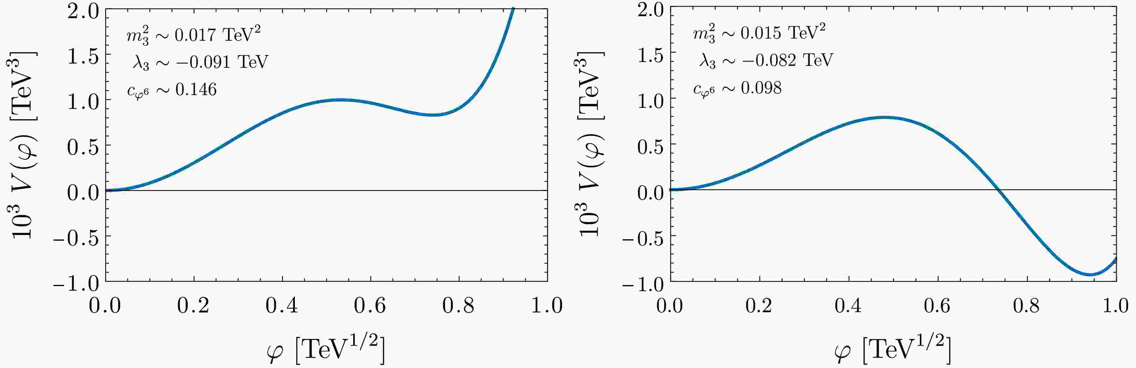
$ \mathbb{Z}_2 $ symmetry$ \varphi\to-\varphi $ , thus avoiding tadpole terms (see e.g., Fig. 1).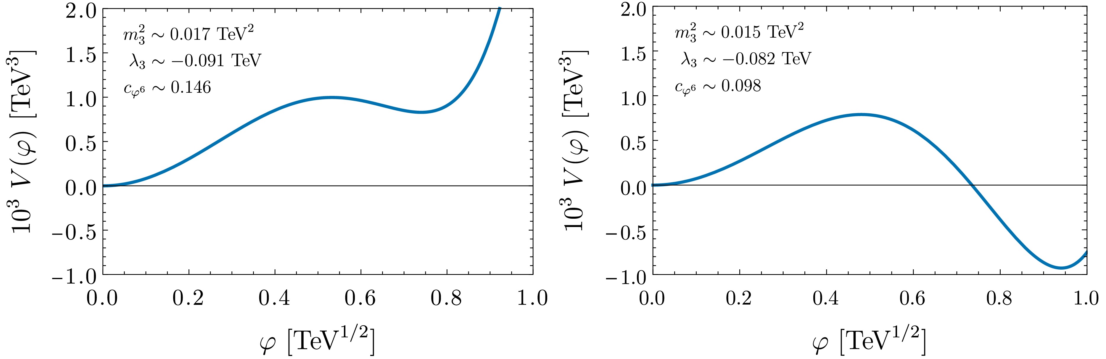
Figure 1. (Color online) Leading scalar potential for different values of the 3D parameters. With slight abuse of notation, φ represents the real component of the complex scalar.
We assume an
$ {\cal{O}}(1) $ Yukawa coupling. For fixed λ, we characterize the parameter space of the model in terms of the physical squared mass ($ m_P^2 $ ) and vacuum expectation value ($ v_P $ ) of ϕ at zero temperature:$ m^2 = \frac{1}{4} (-m_P^2-2 \lambda v_P^2)\,,\quad \frac{c_{\phi^6}}{\Lambda^2} = \frac{1}{3 v_P^4} (m_P^2-2\lambda v_P^2)\,. $

(9) We consider λ as our power counting parameter. The remaining couplings obey different power counting rules in different regions of the parameter space where there are PT
1 . For SM-like values of$ m_P^2 $ and$ v_P $ , we have$ (m / T)^2\sim y^2\sim\lambda $ ,$ c_{\phi^6}\sim\lambda^2 $ [18, 53, 62]. However, for relatively large values of λ and$ m_P^2 $ , we have$ (m/T)^2\sim y\sim\lambda $ ,$ c_{\phi^6}\sim\lambda^2 $ . Within this latter parameter space region, all sum-integrals needed for computing the 3D EFT WCs to order$ \lambda^3 $ , including 3-loop ones, are known2 (see Appendix A). Therefore, a fully consistent study of PT at this order is achievable, which constitutes another major advantage of this model.Hence, in what follows, we consider two benchmark scenarios within this region of the parameter space:
$ \begin{split} & \text{BP1}: (v_P, m_P^2) = (0.5\,\text{TeV}, 0.2\,\text{TeV}^2)\,,\\& \text{BP2}: (v_P, m_P^2) = (0.4\,\text{TeV}, 0.1\,\text{TeV}^2)\,, \end{split} $

(10) and
$ y=0.9 $ in both cases. (For relatively smaller values of y, there is no PT within this regime; for larger ones, SM-like power counting holds.) The region of the parameter space where a PT occurs is very small (occurring for$ -0.5\lesssim\lambda\lesssim 0.3 $ ) and shrinks for larger parameter values, which are also in tension with the assumed EFT cut-off of$ \Lambda=1 $ TeV.The 4D and 3D parameters run following the corresponding renormalization group equations (RGE), which in turn depend on the counterterms (CT). In the 4D theory, the latter are listed below:
$ \delta K_\phi = -\frac{3}{16\pi^2\epsilon}y^2-\frac{1}{128\pi^4\epsilon}\lambda^2, $

(11) $ \delta m^2 = \frac{1}{4\pi^2\epsilon}m^2\lambda + \frac{1}{64\pi^4}\left(-\frac{3}{\epsilon}m^2\lambda^2+\frac{7}{\epsilon^2}m^2\lambda^2\right)\,, $

(12) $ \begin{split} \delta\lambda = & \frac{1}{8 \pi^2\epsilon} \left( 5\lambda^2 + \frac{9}{2}m^2\frac{c_{\phi^6}}{\Lambda^2} \right) + \frac{1}{64\pi^4} \left( - \frac{1}{\epsilon} 16\lambda^3 + \frac{1}{\epsilon^2}25\lambda^3 \right)\,, \end{split}$

(13) $ \delta c_{\phi^6} = \frac{3}{\pi^2\epsilon}\lambda\frac{c_{\phi^6}}{\Lambda^2}\,, $

(14) $ \delta K_\psi = -\frac{3}{32\pi^2\epsilon}y^2, $

(15) $ \delta y = 0 \,, $

(16) where
$ K_\phi $ and$ K_\psi $ are the kinetic terms of the scalar and fermions, respectively. Here,$ \delta K_\psi $ and$ \delta y $ are computed only up to 1-loop because the 2-loop CTs of the fermionic interactions are irrelevant for matching to order$ \lambda^3 $ . In the 3D theory, the CTs are as follows:$ \delta m_3^2 = \frac{1}{8\pi^2\epsilon} \lambda_3^2 \,,\quad \delta\lambda_3 = \frac{9}{8\pi^2\epsilon} \lambda_3 c_{\varphi^6}\,. $

(17) All other terms vanish at order
$ \lambda^3 $ .We refer to Appendix B for the relevant diagrams and for the explicit computations of
$ \delta\lambda $ and$ \delta\lambda_3 $ . Note that 1-loop integrals are not divergent in 3D, and that the squared mass does not renormalize at 3-loops in 4D or 3D. This is because the 3-loop diagrams necessarily scale with$ \lambda c_{\phi^6} $ or$ \lambda^3 $ , which, contrary to$ m^2 $ ($ m_3^2 $ ), have energy dimensions$ -2 $ and$ 0 $ ($ 1 $ and$ 3 $ ) in 4D (3D), respectively.The perturbative solution to the 4D RGEs reads:
$ \begin{split} m^2(\mu) =& m^2 \left[1 + \frac{1}{8\pi^2}(4 \lambda + 3 y^2) \log \frac{\mu}{\Lambda} \right.\\&\left.+\frac{1}{32\pi^4} \lambda^2 \left(14 \log^2 \frac{\mu}{\Lambda} - 5 \log \frac{\mu}{\Lambda}\right)\right]\,, \end{split} $

(18) $ \begin{split} \lambda(\mu) =& \lambda \left[ 1 + \frac{1}{4 \pi^2} (5 \lambda + 3 y^2) \log \frac{\mu}{\Lambda} + \frac{5}{16 \pi^4} \lambda^2\right. \\ &\left. \left( 5 \log^2 \frac{\mu}{\Lambda} - 3 \log \frac{\mu}{\Lambda} \right) \right] + \frac{9}{8 \pi^2} m^2 \frac{c_{\phi^6}}{\Lambda^2} \log \frac{\mu}{\Lambda} \,, \end{split} $

(19) $ y(\mu)= y \left[ 1 + \frac{3}{8 \pi^2} y^2 \log \frac{\mu}{\Lambda} + \frac{1}{256 \pi^4} \lambda^2 \log \frac{\mu}{\Lambda}\right]\,, $

(20) $ c_{\phi^6}(\mu) = c_{\phi^6} \left[ 1 + \frac{6}{ \pi^2} \lambda \log \frac{\mu}{\Lambda} \right] \,, $

(21) where the couplings on the right-hand side of the equations are implicitly evaluated at Λ. We note that the running of the WCs above also encodes the running of ϕ and ψ, as they have been canonically normalized by their corresponding RGEs —this is precisely why, before canonical normalization, y runs despite
$ \delta y = 0 $ in Eq. (16). Some of these results can be cross-checked against$\mathtt{PyR@TE 3}$ [66], where we observe complete agreement.In order to determine the EFT WCs in terms of 4D couplings, we compute the hard region expansion of off-shell correlators involving the zeroth mode of ϕ in the Euclidean version of Eq. (1) in the static limit
$ P^2=(0,\mathbf{p}^2) $ at order$ \lambda^3 $ . This includes 1-loop diagrams for dimension-6 terms, up to 2-loop diagrams for the quartic and up to 3-loop diagrams for the squared mass. Subsequently, we match the result onto the tree-level counterpart in the EFT; see Appendix C. This computation comprises the most demanding part of this work.To simplify the expressions below, we introduce the following notation [5]:
$ L_b = L_b(\mu) \equiv 2 \log \frac{e^{\gamma_E} \mu}{4 \pi T} \,,\quad L_f = L_f(\mu) \equiv 2 \log \frac{e^{\gamma_E} \mu}{\pi T} \,, $

(22) where μ is the matching scale. All numerical constants and special functions that appear in the solution to sum-integrals are defined in Appendix A.
We first determine how the 4D zeroth mode of ϕ is related to φ in the 3D EFT. This is given by the kinetic-term-matching equation:
$ K_3 = 1 + \frac{3}{16 \pi^2} y^2 L_f + \frac{1}{768 \pi^4} \lambda^2 \left(19 + 12 L_b \right) \,. $

(23) Then, we canonically normalize the 3D EFT through
$ \varphi \to \varphi / \sqrt{K_3} $ . With a slight abuse of notation, we use the same names for the canonically normalized WCs and for the unnormalized WCs shown in Eq. (2). The rest of the (normalized) matching equations read:$ \begin{split} m_3^2 = & m^2 + \lambda \left[\frac{1}{3}T^2 - \frac{1}{4 \pi^2} m^2 L_b + \frac{\zeta(3)}{32 \pi^4 T^2} m^4\right]+ y^2 \left( \frac{1}{4}T^2 - \frac{3}{16 \pi^2} m^2 L_f \right) + \frac{c_{\phi^6}}{\Lambda^2} \left( \frac{1}{8}T^4 - \frac{3}{16\pi^2} m^2 T^2 L_b\right) - \frac{1}{32 \pi^2} \lambda y^2 T^2 \left( 3 L_b + L_f \right) \\ & + \frac{1}{16 \pi^2} \lambda^2 \left[ T^2 \left( L_f - \frac{1}{3} L_b + 4 \log\pi - \frac{24 \zeta'(2)}{\pi^2} {+ \color{blue}\frac{2}{\epsilon}\,} \right) + \frac{1}{4 \pi^2}m^2 \left( 7 L_b^2 + 5 L_b + \frac{89}{12} + \frac{4 \zeta(3)}{3} \right) \right] \\ & + \frac{1}{16 \pi^2} \lambda\frac{c_{\phi^6}}{\Lambda^2} T^4 \left[\frac{3}{2} \left( L_b + L_f \right) +\frac{29}{10} - \frac{36 \zeta '(2)}{\pi ^2} + 360 \zeta'(-3) - 3 \gamma + 6 \log\pi + {\color{blue}\frac{3}{\epsilon}\,} \right] \\ & + \frac{1}{128 \pi^4}\lambda^3 T^2 \left[ 2 C_{b} - 10 C_{s} - \frac{85}{3} L_b^2 - 5 L_f^2 + L_b \left( \frac{89}{3} + \frac{240 \zeta'(2)}{\pi^2} - \frac{80 \gamma}{3} {\color{blue}- \frac{20}{\epsilon}\,} \right) \right. \\ & - L_f \left( \frac{29}{3} - \frac{80 \gamma}{3} + 40 \log\pi \right) - \frac{1}{9} \left( 313 \pi^2 + 509 \right) + \frac{4 \zeta(3)}{3} + \left( 41 - 20 \gamma \right) \frac{8 \zeta'(2)}{\pi^2} \\ & - 160 \zeta''(-1) + 8 \gamma \left( 19 \gamma - 2 \right) + \frac{992 \gamma_1}{3} + \frac{4}{3} \left( -29 + 80 \gamma - 60 \log\pi \right) \log\pi ] \,, \end{split} $

(24) $ \begin{split} \lambda_3 &= \lambda T + \frac{c_{\phi^6}}{\Lambda^2} \left(\frac{3}{4}T^3 - \frac{9}{16\pi^2} m^2 T L_b\right) - \frac{5}{8 \pi^2}\lambda^2 \left[T L_b - \frac{\zeta(3)}{4 \pi^2 T} m^2 \right] - \frac{3}{8 \pi^2}\lambda y^2 T L_f\\ &+ \frac{9}{8 \pi^2} \lambda \frac{c_{\phi^6}}{\Lambda^2} T^3 \left[2 \log 2\pi - \frac{12\zeta'(2)}{\pi^2} {+ \color{blue}\frac{1}{\epsilon}\,} \right] + \frac{\lambda^3 T}{128 \pi^4} \left[50 L_b^2 + 60 L_b + \frac{269}{3} + \frac{20 \zeta(3)}{3} \right] \,, \end{split} $

(25) $ \begin{split} c_{\varphi^6} =\;& \frac{c_{\phi^6}}{\Lambda^2} T^2 - \frac{3}{\pi^2 } \lambda \frac{c_{\phi^6}}{\Lambda^2} T^2 L_b + \frac{7 \zeta(3)}{24\pi^4} \lambda^3\,,\\ c_{\partial^2\varphi^4}^{(1)} = \;& r_{\partial^2\varphi^4}^{(2)} =-\frac{\zeta(3)}{48 \pi^4 T} \lambda^2\,; \end{split} $

(26) while all others vanish at order
$ \lambda^3 $ .Note that, upon replacing
$ \lambda_3 $ and$ c_{\varphi_6} $ in Eq. (17) with their matching expressions in Eqs. (25) and (26), we obtain:$ \delta m_3^2 = \frac{1}{\epsilon} \left[ \frac{1}{16 \pi^2} \left( 2 \lambda^2 T^2 + 3 \lambda\frac{ c_{\phi^6}}{\Lambda^2} T^4 \right) - \frac{5}{32 \pi^4} \lambda^3 T^2 L_b \right] \,, $

(27) $ \delta\lambda_3 = \frac{9}{8 \pi^2 \epsilon} \lambda \frac{c_{\phi^6}}{\Lambda^2} T^3\,. $

(28) These are precisely the leftover divergences, shown in blue, in Eqs. (24) and (25); all others are UV poles that are renormalized away. We remark that this is the result of a large number of cancellations, involving different loop orders, with and without CTs (see Appendix C). It therefore constitutes an important cross-check for the matching. In particular, all double poles, of the form
$ 1/\epsilon^2 $ , vanish.The expressions above get further corrections from light loops, captured by the Coleman-Weinberg potential (see Appendix D). Adding these to Eqs. (24) and (25) and taking into account the dependence of
$ m^2 $ , λ, y, and$ c_{\phi^6} $ on μ given in Eqs. (18)–(21), the potential becomes renormalization-scale invariant up to order$ \lambda^3 $ , as shown in Fig. 2. (This is not exact in the case of$ m_3^2 $ because we neglect the 3-loop Coleman-Weinberg potential; however, the dependence of the renormalization scale is minute and becomes generally imperceptible in numerical results). For$ \lambda\sim -0.5 $ , ignoring both 4D and 3D running introduces renormalization-scale dependence of approximately 20% in$ \lambda_3 $ and of approximately 40% in$ c_{\varphi^6} $ . The rest of the action is trivially independent of μ.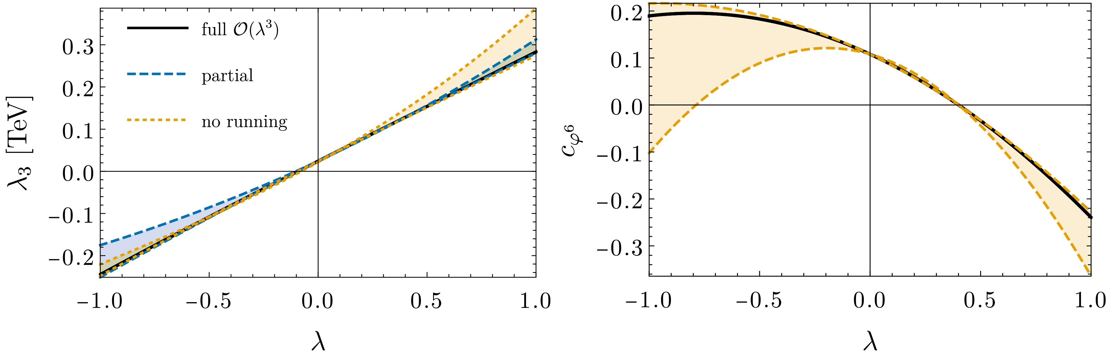
Figure 2. (Color online)
$ \lambda_3 $ (left) and$ c_{\varphi^6} $ (right) for$ T=\Lambda/\pi $ as a function of λ in BP1, including both the running of 4D parameters and Coleman-Weinberg corrections (solid black), only the former (dashed blue) and none (dotted orange). The bands represent variations of the renormalization scale μ in the range$ \mu\in [\overline{T}/2, 2\overline{T}] $ , with$ \overline{T} = \Lambda e^{-\gamma_E} $ .As an example, let us show how
$ \lambda_3 $ , as determined from Eq. (25), becomes scale-independent upon inserting the running of the UV WCs in Eqs. (18)–(21) and the effective potential. Neglecting$ {\cal{O}}(\lambda^4) $ corrections, we have:$ \begin{split} \dot{\lambda}^{\rm full}_3 &\equiv \dot{\lambda}_3 + \dot{\lambda}_3^\text{eff} = \mu\frac{\rm d}{{\rm d}\mu} \left[ \lambda_3 - \frac{9}{4 \pi^2} \left(1 + 2\log\mu \right) c_{\varphi^6} \lambda_3 \right] \\& = \dot{\lambda} T + \frac{3}{4} \frac{\dot{c}_{\phi^6}}{\Lambda^2} T^3 - \frac{9}{8 \pi^2} \frac{c_{\phi^6}}{\Lambda^2} m^2 T \\&- \frac{5}{2 \pi^2} \dot{\lambda} \lambda T \left( \log\mu + \log \frac{e^\gamma}{4 \pi T} \right) - \frac{5}{4 \pi^2} \lambda^2 T \hphantom= - \frac{3}{4 \pi^2} \lambda y^2 T \\& + \frac{1}{16 \pi^4} \lambda^3 T \left[50 \log\mu + \left(50 \log \frac{e^\gamma}{4 \pi T} + 15 \right) \right] - \frac{9}{2 \pi^2} \frac{c_{\phi^6}}{\Lambda^2} \lambda T^3 \\ &= \left( \frac{5}{4\pi^2}\lambda^2 + \frac{9}{8 \pi^2} \frac{c_{\phi^6}}{\Lambda^2} m^2 + \frac{3}{4 \pi^2} \lambda y^2 - \frac{15}{16 \pi^4} \lambda^3 \right) T + \frac{9}{2 \pi^2} \frac{c_{\phi^6}}{\Lambda^2} \lambda T^3 \\ \hphantom= &- \frac{9}{8 \pi^2} \frac{c_{\phi^6}}{\Lambda^2} m^2 T - \frac{5}{4 \pi^2} \lambda^2 T - \frac{25}{8 \pi^4} \lambda^3 T \left( \log\mu + \log \frac{e^\gamma}{4 \pi T} \right) \\ \hphantom= & - \frac{3}{4 \pi^2} \lambda y^2 T+ \frac{1}{16 \pi^4} \lambda^3 T \left[50 \log\mu + \left(50 \log \frac{e^\gamma}{4 \pi T} + 15 \right) \right] \\&- \frac{9}{2 \pi^2} \frac{c_{\phi^6}}{\Lambda^2} \lambda T^3 = 0\,, \end{split} $

(29) where
$ \lambda_3^{\text{eff}} $ is the effective potential contribution to the quartic coupling, which can be read directly from Eq. (D10), and the dot represents$ \mu \dfrac{\rm d}{\rm d\mu} $ .Non-local terms in the effective potential spoil the power counting in λ. In what follows, we include the 1-loop effective potential in the
$ \lambda^2 $ and count$ \log{\mu/m_3} $ as order$ \lambda^0 $ for the 2-loop part. (The latter ones are negligible in any case; their effect is mainly to cancel the scale dependence of physical parameters.) -
We consider a model consisting of a complex scalar field ϕ with global
$ U(1)_X $ charge$ X=1 $ and$ N=3 $ fermions$ \psi_L $ and$ \psi_R $ with charges$ X=1 $ and$ X=0 $ , respectively, with the following Lagrangian in Minkowski space-time:$ \begin{split} {\cal{L}}_{4} &= \partial_\mu\phi^\dagger \partial^\mu\phi - m^2 \phi^\dagger\phi - \lambda(\phi^\dagger\phi)^2 - \frac{c_{\phi^6}}{\Lambda^2}(\phi^\dagger\phi)^3 \\ &\hphantom= + i\overline{\psi_L}{\not {\partial}}\psi_L + i\overline{\psi_R}\not {\partial}\psi_R - y (\phi \overline{\psi_L}\psi_R+\text{h.c.})\,, \end{split} $
(1) where Λ is some energy cut-off. We will work in TeV units throughout and assume that
$ \Lambda=1 $ TeV without loss of generality.The high-temperature limit of this theory is described by a 3D EFT involving only the (loop-corrected) zeroth mode of ϕ, which we call φ. The most general off-shell parametrization of the corresponding Lagrangian up to dimension-6 operators (in 4D units), built using
$\mathtt{ABC4EFT}$ [65], reads as follows in Euclidean space:$ \begin{split} {\cal{L}}_{\text{EFT}} = &K_3\partial_{\mu} \varphi^{\dagger} \partial^{\mu} \varphi + m_3^2 \varphi^{\dagger} \varphi + \lambda_3 (\varphi^{\dagger} \varphi)^2 \\&+ c_{\varphi^6}(\varphi^{\dagger} \varphi)^3 + c^{(1)}_{\partial^2 \varphi^4} (\varphi^{\dagger} \varphi) (\partial_{\mu} \varphi^{\dagger} \partial^{\mu} \varphi) \hphantom= \\ &+ r^{(2)}_{\partial^2 \varphi^4} \left[(\varphi^{\dagger} \varphi) (\partial^2 \varphi^{\dagger} \varphi) + \text{h.c.}\right] \\&+ r^{(3)}_{\partial^2 \varphi^4} \left[i(\varphi^{\dagger} \varphi) (\partial^2 \varphi^{\dagger} \varphi) + \text{h.c.}\right] + r_{\partial^4 \varphi^2} \varphi^{\dagger} \partial^4 \varphi\,. \end{split} $
(2) The WCs named with r are redundant on-shell; that is, they can be removed via field redefinitions. Upon canonically normalizing
$ {\cal{L}}_\text{EFT} $ (such that$ K_3=1 $ ), the equation of motion of φ up to dimension 4 is$ \partial^2 \varphi = m_3^2 \varphi + 2\lambda_3 (\varphi^{\dagger} \varphi)\varphi\,, $
(3) from which the reduction of the redundant operators up to dimension 6 can be deduced as
$ {\cal{R}}^{(2)}_{\partial^2 \varphi^4} = (\varphi^{\dagger} \varphi) (\partial^2 \varphi^{\dagger} \varphi) + \text{h.c.} = 2 m_3^2(\varphi^{\dagger} \varphi)^2 + 4\lambda_3 (\varphi^{\dagger} \varphi)^3 \,, $
(4) $ {\cal{R}}^{(3)}_{\partial^2 \varphi^4} = i(\varphi^{\dagger} \varphi) (\partial^2 \varphi^{\dagger} \varphi) + \text{h.c.} = 0 \,, $
(5) $ {\cal{R}}_{\partial^4 \varphi^2} = (\varphi^{\dagger} \partial^4 \varphi) = m_3^4 (\varphi^{\dagger} \varphi) + 4\lambda_3 m_3^2 (\varphi^{\dagger} \varphi)^2 + 4\lambda^2_3 (\varphi^{\dagger} \varphi)^3 \,. $
(6) Hence, the physical Lagrangian reads
$ \begin{split} {\cal{L}}^{\text{phys}}_{\text{EFT}} =& \partial_{\mu} \varphi^{\dagger} \partial^{\mu} \varphi + m'_3{}^2 \varphi^{\dagger} \varphi + \lambda'_3 (\varphi^{\dagger} \varphi)^2 \\&+ c'_{\varphi^6}(\varphi^{\dagger} \varphi)^3 + c'_{\partial^2 \varphi^4} (\varphi^{\dagger} \varphi) (\partial_{\mu} \varphi^{\dagger} \partial^{\mu} \varphi) \,, \end{split}$
(7) and the above WCs are connected to those in Eq. (2) by
$ \begin{split} &m'_3{}^2 = m_3^2 + m_3^4 r_{\partial^4 \varphi^2} \,, \quad \lambda'_3 = \lambda_3 + 2m_3^2 r^{(2)}_{\partial^2 \varphi^4} + 4\lambda_3 m_3^2 r_{\partial^4 \varphi^2} \,, \\ &c'_{\varphi^6} = c_{\varphi^6} + 4\lambda_3 r^{(2)}_{\partial^2 \varphi^4} + 4\lambda^2_3 r_{\partial^4 \varphi^2} \,, \quad c'_{\partial^2 \varphi^4} = c_{\partial^2 \varphi^4} \,. \end{split} $
(8) This model is appealing in the following respects: (i) it resembles the Higgs sector of the SMEFT, while being significantly simpler; (ii) it is not as simple as the real scalar model [50], which presents no physical derivative interactions beyond the kinetic term; (iii) it can deliver two minima separated by a barrier while maintaining
$ \mathbb{Z}_2 $ symmetry$ \varphi\to-\varphi $ , thus avoiding tadpole terms (see e.g., Fig. 1).
Figure 1. (Color online) Leading scalar potential for different values of the 3D parameters. With slight abuse of notation, φ represents the real component of the complex scalar.
We assume an
$ {\cal{O}}(1) $ Yukawa coupling. For fixed λ, we characterize the parameter space of the model in terms of the physical squared mass ($ m_P^2 $ ) and vacuum expectation value ($ v_P $ ) of ϕ at zero temperature:$ m^2 = \frac{1}{4} (-m_P^2-2 \lambda v_P^2)\,,\quad \frac{c_{\phi^6}}{\Lambda^2} = \frac{1}{3 v_P^4} (m_P^2-2\lambda v_P^2)\,. $
(9) We consider λ as our power counting parameter. The remaining couplings obey different power counting rules in different regions of the parameter space where there are PT
1 . For SM-like values of$ m_P^2 $ and$ v_P $ , we have$ (m / T)^2\sim y^2\sim\lambda $ ,$ c_{\phi^6}\sim\lambda^2 $ [18, 53, 62]. However, for relatively large values of λ and$ m_P^2 $ , we have$ (m/T)^2\sim y\sim\lambda $ ,$ c_{\phi^6}\sim\lambda^2 $ . Within this latter parameter space region, all sum-integrals needed for computing the 3D EFT WCs to order$ \lambda^3 $ , including 3-loop ones, are known2 (see Appendix A). Therefore, a fully consistent study of PT at this order is achievable, which constitutes another major advantage of this model.Hence, in what follows, we consider two benchmark scenarios within this region of the parameter space:
$ \begin{split} & \text{BP1}: (v_P, m_P^2) = (0.5\,\text{TeV}, 0.2\,\text{TeV}^2)\,,\\& \text{BP2}: (v_P, m_P^2) = (0.4\,\text{TeV}, 0.1\,\text{TeV}^2)\,, \end{split} $
(10) and
$ y=0.9 $ in both cases. (For relatively smaller values of y, there is no PT within this regime; for larger ones, SM-like power counting holds.) The region of the parameter space where a PT occurs is very small (occurring for$ -0.5\lesssim\lambda\lesssim 0.3 $ ) and shrinks for larger parameter values, which are also in tension with the assumed EFT cut-off of$ \Lambda=1 $ TeV.The 4D and 3D parameters run following the corresponding renormalization group equations (RGE), which in turn depend on the counterterms (CT). In the 4D theory, the latter are listed below:
$ \delta K_\phi = -\frac{3}{16\pi^2\epsilon}y^2-\frac{1}{128\pi^4\epsilon}\lambda^2, $
(11) $ \delta m^2 = \frac{1}{4\pi^2\epsilon}m^2\lambda + \frac{1}{64\pi^4}\left(-\frac{3}{\epsilon}m^2\lambda^2+\frac{7}{\epsilon^2}m^2\lambda^2\right)\,, $
(12) $ \begin{split} \delta\lambda = & \frac{1}{8 \pi^2\epsilon} \left( 5\lambda^2 + \frac{9}{2}m^2\frac{c_{\phi^6}}{\Lambda^2} \right) + \frac{1}{64\pi^4} \left( - \frac{1}{\epsilon} 16\lambda^3 + \frac{1}{\epsilon^2}25\lambda^3 \right)\,, \end{split}$
(13) $ \delta c_{\phi^6} = \frac{3}{\pi^2\epsilon}\lambda\frac{c_{\phi^6}}{\Lambda^2}\,, $
(14) $ \delta K_\psi = -\frac{3}{32\pi^2\epsilon}y^2, $
(15) $ \delta y = 0 \,, $
(16) where
$ K_\phi $ and$ K_\psi $ are the kinetic terms of the scalar and fermions, respectively. Here,$ \delta K_\psi $ and$ \delta y $ are computed only up to 1-loop because the 2-loop CTs of the fermionic interactions are irrelevant for matching to order$ \lambda^3 $ . In the 3D theory, the CTs are as follows:$ \delta m_3^2 = \frac{1}{8\pi^2\epsilon} \lambda_3^2 \,,\quad \delta\lambda_3 = \frac{9}{8\pi^2\epsilon} \lambda_3 c_{\varphi^6}\,. $
(17) All other terms vanish at order
$ \lambda^3 $ .We refer to Appendix B for the relevant diagrams and for the explicit computations of
$ \delta\lambda $ and$ \delta\lambda_3 $ . Note that 1-loop integrals are not divergent in 3D, and that the squared mass does not renormalize at 3-loops in 4D or 3D. This is because the 3-loop diagrams necessarily scale with$ \lambda c_{\phi^6} $ or$ \lambda^3 $ , which, contrary to$ m^2 $ ($ m_3^2 $ ), have energy dimensions$ -2 $ and$ 0 $ ($ 1 $ and$ 3 $ ) in 4D (3D), respectively.The perturbative solution to the 4D RGEs reads:
$ \begin{split} m^2(\mu) =& m^2 \left[1 + \frac{1}{8\pi^2}(4 \lambda + 3 y^2) \log \frac{\mu}{\Lambda} \right.\\&\left.+\frac{1}{32\pi^4} \lambda^2 \left(14 \log^2 \frac{\mu}{\Lambda} - 5 \log \frac{\mu}{\Lambda}\right)\right]\,, \end{split} $
(18) $ \begin{split} \lambda(\mu) =& \lambda \left[ 1 + \frac{1}{4 \pi^2} (5 \lambda + 3 y^2) \log \frac{\mu}{\Lambda} + \frac{5}{16 \pi^4} \lambda^2\right. \\ &\left. \left( 5 \log^2 \frac{\mu}{\Lambda} - 3 \log \frac{\mu}{\Lambda} \right) \right] + \frac{9}{8 \pi^2} m^2 \frac{c_{\phi^6}}{\Lambda^2} \log \frac{\mu}{\Lambda} \,, \end{split} $
(19) $ y(\mu)= y \left[ 1 + \frac{3}{8 \pi^2} y^2 \log \frac{\mu}{\Lambda} + \frac{1}{256 \pi^4} \lambda^2 \log \frac{\mu}{\Lambda}\right]\,, $
(20) $ c_{\phi^6}(\mu) = c_{\phi^6} \left[ 1 + \frac{6}{ \pi^2} \lambda \log \frac{\mu}{\Lambda} \right] \,, $
(21) where the couplings on the right-hand side of the equations are implicitly evaluated at Λ. We note that the running of the WCs above also encodes the running of ϕ and ψ, as they have been canonically normalized by their corresponding RGEs —this is precisely why, before canonical normalization, y runs despite
$ \delta y = 0 $ in Eq. (16). Some of these results can be cross-checked against$\mathtt{PyR@TE 3}$ [66], where we observe complete agreement.In order to determine the EFT WCs in terms of 4D couplings, we compute the hard region expansion of off-shell correlators involving the zeroth mode of ϕ in the Euclidean version of Eq. (1) in the static limit
$ P^2=(0,\mathbf{p}^2) $ at order$ \lambda^3 $ . This includes 1-loop diagrams for dimension-6 terms, up to 2-loop diagrams for the quartic and up to 3-loop diagrams for the squared mass. Subsequently, we match the result onto the tree-level counterpart in the EFT; see Appendix C. This computation comprises the most demanding part of this work.To simplify the expressions below, we introduce the following notation [5]:
$ L_b = L_b(\mu) \equiv 2 \log \frac{e^{\gamma_E} \mu}{4 \pi T} \,,\quad L_f = L_f(\mu) \equiv 2 \log \frac{e^{\gamma_E} \mu}{\pi T} \,, $
(22) where μ is the matching scale. All numerical constants and special functions that appear in the solution to sum-integrals are defined in Appendix A.
We first determine how the 4D zeroth mode of ϕ is related to φ in the 3D EFT. This is given by the kinetic-term-matching equation:
$ K_3 = 1 + \frac{3}{16 \pi^2} y^2 L_f + \frac{1}{768 \pi^4} \lambda^2 \left(19 + 12 L_b \right) \,. $
(23) Then, we canonically normalize the 3D EFT through
$ \varphi \to \varphi / \sqrt{K_3} $ . With a slight abuse of notation, we use the same names for the canonically normalized WCs and for the unnormalized WCs shown in Eq. (2). The rest of the (normalized) matching equations read:$ \begin{split} m_3^2 = & m^2 + \lambda \left[\frac{1}{3}T^2 - \frac{1}{4 \pi^2} m^2 L_b + \frac{\zeta(3)}{32 \pi^4 T^2} m^4\right]+ y^2 \left( \frac{1}{4}T^2 - \frac{3}{16 \pi^2} m^2 L_f \right) + \frac{c_{\phi^6}}{\Lambda^2} \left( \frac{1}{8}T^4 - \frac{3}{16\pi^2} m^2 T^2 L_b\right) - \frac{1}{32 \pi^2} \lambda y^2 T^2 \left( 3 L_b + L_f \right) \\ & + \frac{1}{16 \pi^2} \lambda^2 \left[ T^2 \left( L_f - \frac{1}{3} L_b + 4 \log\pi - \frac{24 \zeta'(2)}{\pi^2} {+ \color{blue}\frac{2}{\epsilon}\,} \right) + \frac{1}{4 \pi^2}m^2 \left( 7 L_b^2 + 5 L_b + \frac{89}{12} + \frac{4 \zeta(3)}{3} \right) \right] \\ & + \frac{1}{16 \pi^2} \lambda\frac{c_{\phi^6}}{\Lambda^2} T^4 \left[\frac{3}{2} \left( L_b + L_f \right) +\frac{29}{10} - \frac{36 \zeta '(2)}{\pi ^2} + 360 \zeta'(-3) - 3 \gamma + 6 \log\pi + {\color{blue}\frac{3}{\epsilon}\,} \right] \\ & + \frac{1}{128 \pi^4}\lambda^3 T^2 \left[ 2 C_{b} - 10 C_{s} - \frac{85}{3} L_b^2 - 5 L_f^2 + L_b \left( \frac{89}{3} + \frac{240 \zeta'(2)}{\pi^2} - \frac{80 \gamma}{3} {\color{blue}- \frac{20}{\epsilon}\,} \right) \right. \\ & - L_f \left( \frac{29}{3} - \frac{80 \gamma}{3} + 40 \log\pi \right) - \frac{1}{9} \left( 313 \pi^2 + 509 \right) + \frac{4 \zeta(3)}{3} + \left( 41 - 20 \gamma \right) \frac{8 \zeta'(2)}{\pi^2} \\ & - 160 \zeta''(-1) + 8 \gamma \left( 19 \gamma - 2 \right) + \frac{992 \gamma_1}{3} + \frac{4}{3} \left( -29 + 80 \gamma - 60 \log\pi \right) \log\pi ] \,, \end{split} $
(24) $ \begin{split} \lambda_3 &= \lambda T + \frac{c_{\phi^6}}{\Lambda^2} \left(\frac{3}{4}T^3 - \frac{9}{16\pi^2} m^2 T L_b\right) - \frac{5}{8 \pi^2}\lambda^2 \left[T L_b - \frac{\zeta(3)}{4 \pi^2 T} m^2 \right] - \frac{3}{8 \pi^2}\lambda y^2 T L_f\\ &+ \frac{9}{8 \pi^2} \lambda \frac{c_{\phi^6}}{\Lambda^2} T^3 \left[2 \log 2\pi - \frac{12\zeta'(2)}{\pi^2} {+ \color{blue}\frac{1}{\epsilon}\,} \right] + \frac{\lambda^3 T}{128 \pi^4} \left[50 L_b^2 + 60 L_b + \frac{269}{3} + \frac{20 \zeta(3)}{3} \right] \,, \end{split} $
(25) $ \begin{split} c_{\varphi^6} =\;& \frac{c_{\phi^6}}{\Lambda^2} T^2 - \frac{3}{\pi^2 } \lambda \frac{c_{\phi^6}}{\Lambda^2} T^2 L_b + \frac{7 \zeta(3)}{24\pi^4} \lambda^3\,,\\ c_{\partial^2\varphi^4}^{(1)} = \;& r_{\partial^2\varphi^4}^{(2)} =-\frac{\zeta(3)}{48 \pi^4 T} \lambda^2\,; \end{split} $
(26) while all others vanish at order
$ \lambda^3 $ .Note that, upon replacing
$ \lambda_3 $ and$ c_{\varphi_6} $ in Eq. (17) with their matching expressions in Eqs. (25) and (26), we obtain:$ \delta m_3^2 = \frac{1}{\epsilon} \left[ \frac{1}{16 \pi^2} \left( 2 \lambda^2 T^2 + 3 \lambda\frac{ c_{\phi^6}}{\Lambda^2} T^4 \right) - \frac{5}{32 \pi^4} \lambda^3 T^2 L_b \right] \,, $
(27) $ \delta\lambda_3 = \frac{9}{8 \pi^2 \epsilon} \lambda \frac{c_{\phi^6}}{\Lambda^2} T^3\,. $
(28) These are precisely the leftover divergences, shown in blue, in Eqs. (24) and (25); all others are UV poles that are renormalized away. We remark that this is the result of a large number of cancellations, involving different loop orders, with and without CTs (see Appendix C). It therefore constitutes an important cross-check for the matching. In particular, all double poles, of the form
$ 1/\epsilon^2 $ , vanish.The expressions above get further corrections from light loops, captured by the Coleman-Weinberg potential (see Appendix D). Adding these to Eqs. (24) and (25) and taking into account the dependence of
$ m^2 $ , λ, y, and$ c_{\phi^6} $ on μ given in Eqs. (18)–(21), the potential becomes renormalization-scale invariant up to order$ \lambda^3 $ , as shown in Fig. 2. (This is not exact in the case of$ m_3^2 $ because we neglect the 3-loop Coleman-Weinberg potential; however, the dependence of the renormalization scale is minute and becomes generally imperceptible in numerical results). For$ \lambda\sim -0.5 $ , ignoring both 4D and 3D running introduces renormalization-scale dependence of approximately 20% in$ \lambda_3 $ and of approximately 40% in$ c_{\varphi^6} $ . The rest of the action is trivially independent of μ.
Figure 2. (Color online)
$ \lambda_3 $ (left) and$ c_{\varphi^6} $ (right) for$ T=\Lambda/\pi $ as a function of λ in BP1, including both the running of 4D parameters and Coleman-Weinberg corrections (solid black), only the former (dashed blue) and none (dotted orange). The bands represent variations of the renormalization scale μ in the range$ \mu\in [\overline{T}/2, 2\overline{T}] $ , with$ \overline{T} = \Lambda e^{-\gamma_E} $ .As an example, let us show how
$ \lambda_3 $ , as determined from Eq. (25), becomes scale-independent upon inserting the running of the UV WCs in Eqs. (18)–(21) and the effective potential. Neglecting$ {\cal{O}}(\lambda^4) $ corrections, we have:$ \begin{split} \dot{\lambda}^{\rm full}_3 &\equiv \dot{\lambda}_3 + \dot{\lambda}_3^\text{eff} = \mu\frac{\rm d}{{\rm d}\mu} \left[ \lambda_3 - \frac{9}{4 \pi^2} \left(1 + 2\log\mu \right) c_{\varphi^6} \lambda_3 \right] \\& = \dot{\lambda} T + \frac{3}{4} \frac{\dot{c}_{\phi^6}}{\Lambda^2} T^3 - \frac{9}{8 \pi^2} \frac{c_{\phi^6}}{\Lambda^2} m^2 T \\&- \frac{5}{2 \pi^2} \dot{\lambda} \lambda T \left( \log\mu + \log \frac{e^\gamma}{4 \pi T} \right) - \frac{5}{4 \pi^2} \lambda^2 T \hphantom= - \frac{3}{4 \pi^2} \lambda y^2 T \\& + \frac{1}{16 \pi^4} \lambda^3 T \left[50 \log\mu + \left(50 \log \frac{e^\gamma}{4 \pi T} + 15 \right) \right] - \frac{9}{2 \pi^2} \frac{c_{\phi^6}}{\Lambda^2} \lambda T^3 \\ &= \left( \frac{5}{4\pi^2}\lambda^2 + \frac{9}{8 \pi^2} \frac{c_{\phi^6}}{\Lambda^2} m^2 + \frac{3}{4 \pi^2} \lambda y^2 - \frac{15}{16 \pi^4} \lambda^3 \right) T + \frac{9}{2 \pi^2} \frac{c_{\phi^6}}{\Lambda^2} \lambda T^3 \\ \hphantom= &- \frac{9}{8 \pi^2} \frac{c_{\phi^6}}{\Lambda^2} m^2 T - \frac{5}{4 \pi^2} \lambda^2 T - \frac{25}{8 \pi^4} \lambda^3 T \left( \log\mu + \log \frac{e^\gamma}{4 \pi T} \right) \\ \hphantom= & - \frac{3}{4 \pi^2} \lambda y^2 T+ \frac{1}{16 \pi^4} \lambda^3 T \left[50 \log\mu + \left(50 \log \frac{e^\gamma}{4 \pi T} + 15 \right) \right] \\&- \frac{9}{2 \pi^2} \frac{c_{\phi^6}}{\Lambda^2} \lambda T^3 = 0\,, \end{split} $
(29) where
$ \lambda_3^{\text{eff}} $ is the effective potential contribution to the quartic coupling, which can be read directly from Eq. (D10), and the dot represents$ \mu \dfrac{\rm d}{\rm d\mu} $ .Non-local terms in the effective potential spoil the power counting in λ. In what follows, we include the 1-loop effective potential in the
$ \lambda^2 $ and count$ \log{\mu/m_3} $ as order$ \lambda^0 $ for the 2-loop part. (The latter ones are negligible in any case; their effect is mainly to cancel the scale dependence of physical parameters.) -
The fundamental quantity to determine in any PT-related computation is the nucleation rate, which has the following form:
$ \Gamma = A_{\rm{stat}} A_{\rm{dyn}} {\rm e}^{-S_3[\varphi_c]}\,, $

(30) where
$ S_3[\varphi_c] $ is the effective 3D action evaluated at the bounce solution [67], of which it is an extremal,$ A_{\rm{stat}} $ is the statistical pre-factor and$ A_{\rm{dyn}} $ is the dynamical pre-factor [68]. The first pre-factor accounts for equilibrium physics, and the latter captures non-equilibrium effects. In this work, we assume the high-temperature approximation$ \Gamma \thickapprox T^4 {\rm e}^{-S_3[\varphi_c]} $ .Since our aim is to quantify the effect of different matching corrections on PT parameters, for simplicity, we restrict our analyses to PT in the real direction of φ. We take
$ \varphi = (\varphi_1 + {\rm i} \varphi_2)/\sqrt{2} $ and with a little abuse of notation, we use φ to denote$ \varphi_1 $ .We compute
$ S_3[\varphi_c] $ using strict perturbation theory [50]:$ S_3[\varphi_c] = S_3^{(0)}[\varphi_c^{(0)}] + S_3^{(1)}[\varphi_c^{(0)}]\,, $

(31) where
$ S_3^{(0)} $ is the 3D action up to order$ \lambda^2 $ and$ S_3^{(1)} $ stands for the$ {\cal{O}}(\lambda^3) $ corrections. Similarly,$ \varphi_c^{(0)} $ is the spherically-symmetric solution of the Euler-Lagrange equation [67]:$ \ddot{\varphi}_c^{(0)} + \frac{2}{r}\dot{\varphi}_c^{(0)} = V_3'(\varphi_c^{(0)}), $

(32) with boundary conditions
$ \dot{\varphi_c}^{(0)}(0)=0 $ and$ V^{(0)'}(\varphi_\infty^{(0)}) = 0 $ , where$ \varphi_\infty^{(0)} \equiv \lim_{r \to \infty} \varphi^{(0)}(r) $ .We compute
$ \varphi_c^{(0)} $ using${\mathtt{FindBounce}}$ [69]; see Refs. [70–74] for similar dedicated tools. We assume that the PT takes place when the probability$ {\cal{P}}\sim (M_{\rm Pl} / T)^4 \, {\rm e}^{-S_3[\varphi_c]} $ for a single bubble to nucleate within a Hubble horizon volume is$ \sim 1 $ . Numerically, this occurs when$ S_3[\varphi_c]\sim 140 $ [75]. We denote by$ T_* $ the temperature at which this holds.Assuming that the Universe is radiation-dominated at the time of the PT, we define the following PT parameters, relevant for the production of GWs [60].
● Strength parameter (α). It is defined as the ratio of the trace anomaly difference of the energy momentum tensor between the symmetric and broken phases to the energy density of the radiation bath
$ \rho_r(T) = g(T) \pi^2 T^4/30 $ [76]:$ \alpha = \frac{T_*}{\rho_r(T_*)}\left.\Delta \left[ V_3(\varphi) - \frac{T}{4} \frac{\rm d}{{\rm d}T} V_3(\varphi) \right]\right|_{T_*}\,, $

(33) with
$ g(T) $ being the number of relativistic degrees of freedom in the plasma at a given temperature. For the SM, at the time of the transition,$ g(T_*) = 106.75 $ [77].● Inverse duration (
$ \beta/H_* $ ). It is a characteristic timescale of the PT, corresponding to an exponentially growing transition rate as the temperature decreases (or equivalently, after linearising the bounce action with respect to the temperature) [60]:$ \frac{\beta}{H_*} = T_* \frac{{\rm d} S_3[\varphi_c]}{{\rm d} T}\bigg|_{T_*}\,. $

(34) ● Terminal bubble wall velocity (
$ v_\omega $ ). In this work, we use the approximation [78]$ v_w = \begin{cases} \sqrt{\dfrac{T_* \Delta V_3}{\alpha \rho_r}} & \text{for} \quad \sqrt{\dfrac{T_* \Delta V_3}{\alpha \rho_r}} < v_J(\alpha) \\ 1 & \text{for} \quad \sqrt{\dfrac{T_* \Delta V_3}{\alpha \rho_r}} \geq v_J(\alpha) \end{cases}\,,\quad v_J = \dfrac{1}{\sqrt{3}} \dfrac{1 + \sqrt{3 \alpha^2 + 2 \alpha}}{1 + \alpha}\,, $

(35) where
$ \Delta V_3 = V_3(\varphi_T) $ is the difference in the potential between the phases.The bubble wall velocity is determined from non-equilibrium processes, namely the interplay between the pressure between the scalar phases and the friction and back-reaction from the plasma. The precise computation of this parameter is a matter of ongoing study, as it is known to significantly affect the GW production from a FOPT; see Refs. [79–86] and the references therein.
To order
$ \lambda^2 $ , which in particular neglects effective interactions, we show α and$ \beta/H_* $ in Fig. 3.$ T_* $ varies much less, ranging from$ \sim 0.3 (0.2) $ to$ 0.15 (0.1) $ for BP1 (BP2).3 Regarding$ {\cal{O}}(\lambda^3) $ corrections, since our principal goal is to clarify the relative size of 1-loop effects of 3D effective operators versus 2-loop and 3-loop corrections to the mass and quartic coupling, in Fig. 4, we compare only the$ {\cal{O}}(\lambda^3) $ contributions to the above PT parameters.4 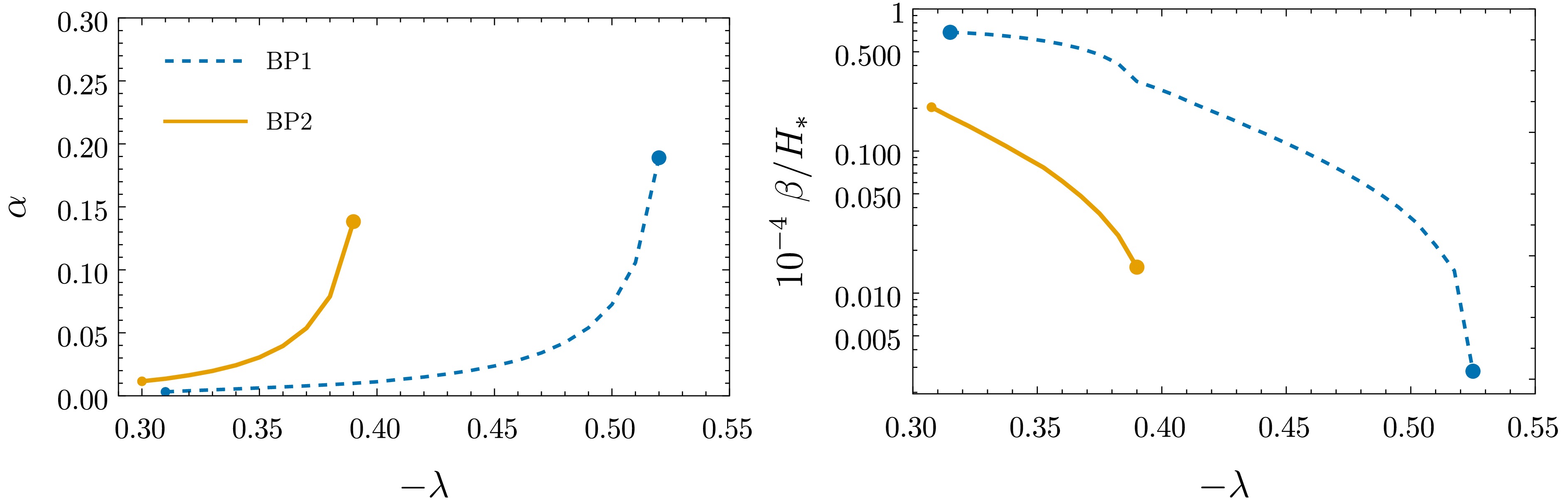
Figure 3. (Color online) α (left) and
$ \beta/H_* $ (right) for BP1 (dashed blue) and BP2 (solid orange). The minimum and maximum values of λ where a PT occurs are marked.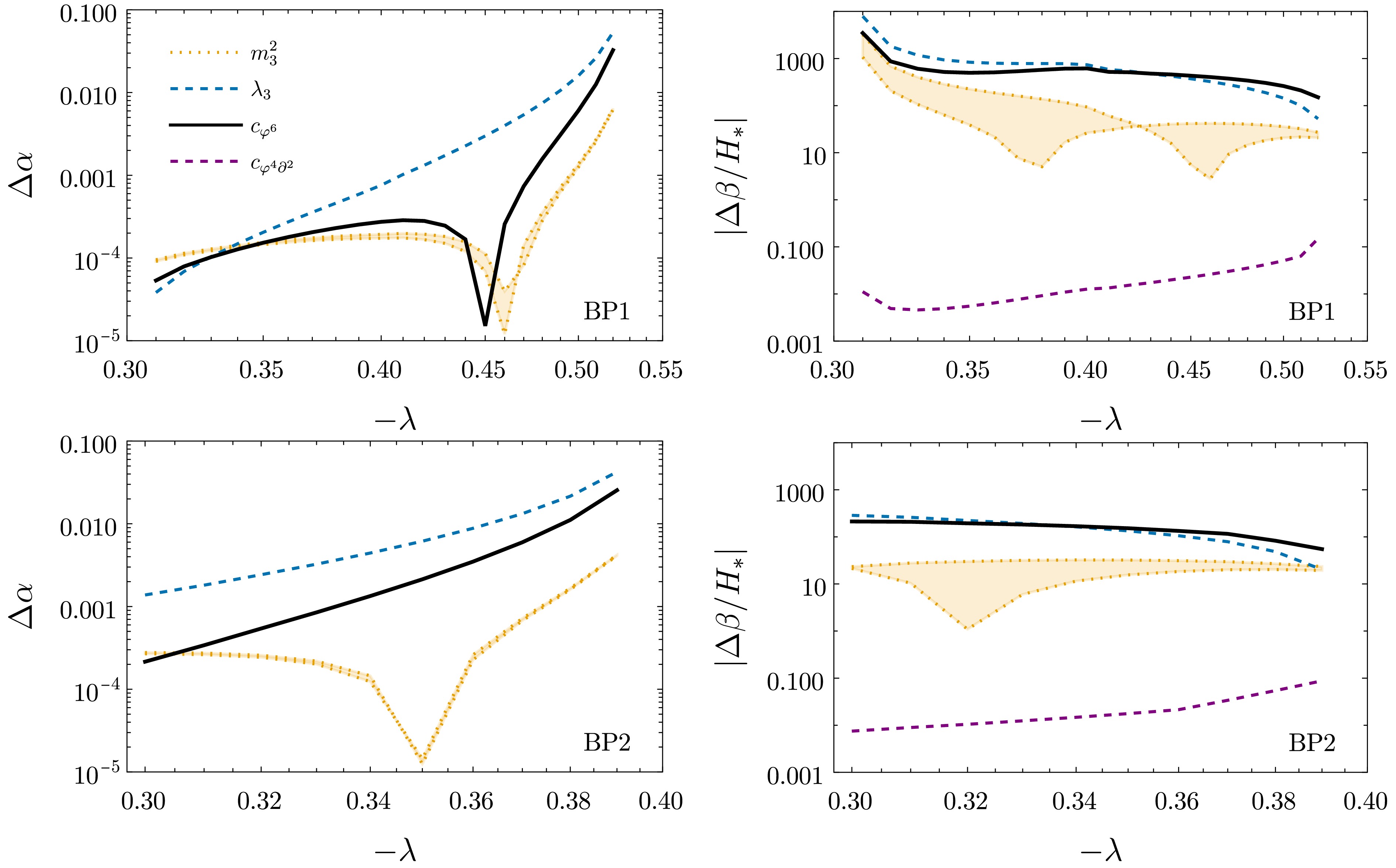
Figure 4. (Color online)
$ {\cal{O}}(\lambda^3) $ contributions from all 3D physical operators to the strength parameter (left) and inverse duration (right) in BP1 (top) and BP2 (bottom). The bands represent variations of the renormalization scale$ \mu\in [\overline{T}/2, 2\overline{T}] $ , with$ \overline{T} = \Lambda {\rm e}^{-\gamma_E} $ .The spiky shape of the
$ m_3^2 $ curves is due to the corresponding$ {\cal{O}}(\lambda^3) $ corrections changing sign. From the plot, we infer that 1-loop corrections from$ \varphi^6 $ compete with the 2-loop quartic and far dominate over the 3-loop mass for sufficiently strong PT (in particular, for those with$ \alpha\gtrsim 0.1 $ , which are the ones that lead to observable GWs [60]). Note that corrections to$ \beta/H_* $ from$ c_{\varphi^6} $ (and from$ \lambda_3 $ ) are negative. This can be understood as follows. In good approximation,$ T_* $ and, therefore, the leading bounce are barely modified upon the introduction of$ {\cal{O}}(\lambda^3) $ corrections. Consequently,$ \begin{split} \frac{\beta}{H_*} & =T_* \frac{\rm d}{{\rm d} T}\left(S_3^{(0)}[\varphi_c^{(0)}]+S_3^{(1)}[\varphi_c^{(0)}]\right)\bigg|_{T_*}\\& \thickapprox \frac{\beta^{(0)}}{H_*} + T_*\frac{{\rm d}S_3^{(1)}[\varphi_c^{(0)}]}{{\rm d}T}\bigg|_{T_*} \,, \end{split}$

(36) where
$ \beta^{(0)}/H_* $ is the value of$ \beta/H_* $ computed without$ {\cal{O}}(\lambda^3) $ corrections and the remainder is the correction we are interested in. Now, since$ T_* $ and$ \varphi_c^{(0)} $ are fixed, all the dependence on T is encoded in the WCs. For the case of$ c_{\varphi^6} $ , we have$ \Delta\frac{\beta}{H_*} = T_*\frac{{\rm d}S_3^{(1)}[\varphi_c^{(0)}]}{{\rm d}T}\bigg|_{T_*} \thickapprox 4\pi T_* \int {\rm d}r r^2 [\varphi_c^{(0)}(r)]^6 \; \frac{1}{8} \frac{{\rm d}c_{\varphi^6}}{{\rm d} T}\bigg|_{T_*}\,, $

(37) which is negative for
$ \begin{split} \frac{{\rm d}c_{\varphi^6}}{{\rm d}T}\bigg|_{T_*} &= \frac{\rm d}{{\rm d}T}\left[\frac{6}{\pi^2} \left(\log{\frac{4\pi T}{\Lambda}}-\gamma_E\right) \lambda c_{\phi^6} T^2 + \frac{7 \zeta(3)}{24\pi^4}\lambda^3\right]\\ &= \frac{6}{\pi^2}\left(1-2\gamma_E+2\log{\frac{4\pi T}{\Lambda}}\right) \lambda c_{\phi^6}T <0\\& \Rightarrow T > \frac{e^{\gamma_E-\frac{1}{2}}}{4\pi}\Lambda < 0.1\; \text{TeV},\, \end{split} $

(38) for
$ \Lambda=1 $ TeV, and therefore, this correction is negative for all temperatures of interest. This implies that, for$ \lambda\gtrsim 0.5 $ , there is no PT within BP1, because the correction to$ \beta/H_* $ makes it negative.To conclude this analysis, we show the impact of
$ {\cal{O}}(\lambda^3) $ corrections in the GW spectrum of two different parameter space points in BP1 and BP2 computed using${\mathtt{PTPlot}}$ [60, 88]; see Fig. 5. It is apparent that 1-loop dimension-6 corrections can significantly dominate over 2-loop and 3-loop corrections on lower-dimensional interactions.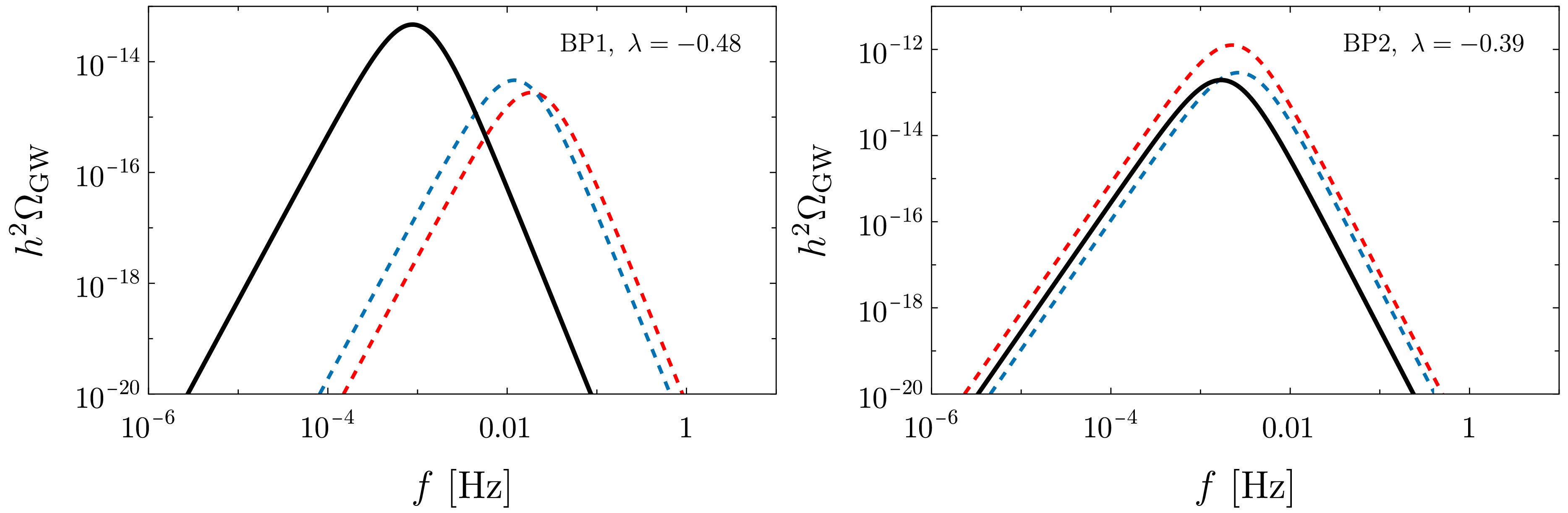
Figure 5. (Color online) GW stochastic background generated during a PT computed at order
$ \lambda^2 $ (dashed red), including 2-loop and 3-loop corrections from the mass and the quartic (dashed blue) and with 1-loop effective-operator corrections (solid black) in BP1 (left) and BP2 (right). -
The fundamental quantity to determine in any PT-related computation is the nucleation rate, which has the following form:
$ \Gamma = A_{\rm{stat}} A_{\rm{dyn}} e^{-S_3[\varphi_c]}\,, $
(30) where
$ S_3[\varphi_c] $ is the effective 3D action evaluated at the bounce solution [67], of which it is an extremal,$ A_{\rm{stat}} $ is the statistical pre-factor and$ A_{\rm{dyn}} $ is the dynamical pre-factor [68]. The first pre-factor accounts for equilibrium physics, and the latter captures non-equilibrium effects. In this work, we assume the high-temperature approximation$ \Gamma \thickapprox T^4 e^{-S_3[\varphi_c]} $ .Since our aim is to quantify the effect of different matching corrections on PT parameters, for simplicity, we restrict our analyses to PT in the real direction of φ. We take
$ \varphi = (\varphi_1 + i \varphi_2)/\sqrt{2} $ and with a little abuse of notation, we use φ to denote$ \varphi_1 $ .We compute
$ S_3[\varphi_c] $ using strict perturbation theory [50]:$ S_3[\varphi_c] = S_3^{(0)}[\varphi_c^{(0)}] + S_3^{(1)}[\varphi_c^{(0)}]\,, $
(31) where
$ S_3^{(0)} $ is the 3D action up to order$ \lambda^2 $ and$ S_3^{(1)} $ stands for the$ {\cal{O}}(\lambda^3) $ corrections. Similarly,$ \varphi_c^{(0)} $ is the spherically-symmetric solution of the Euler-Lagrange equation [67]:$ \ddot{\varphi}_c^{(0)} + \frac{2}{r}\dot{\varphi}_c^{(0)} = V_3'(\varphi_c^{(0)}), $
(32) with boundary conditions
$ \dot{\varphi_c}^{(0)}(0)=0 $ and$ V^{(0)'}(\varphi_\infty^{(0)}) = 0 $ , where$ \varphi_\infty^{(0)} \equiv \lim_{r \to \infty} \varphi^{(0)}(r) $ .We compute
$ \varphi_c^{(0)} $ using${\mathtt{FindBounce}}$ [69]; see Refs. [70–74] for similar dedicated tools. We assume that the PT takes place when the probability$ {\cal{P}}\sim (M_{\rm Pl} / T)^4 \, {\rm e}^{-S_3[\varphi_c]} $ for a single bubble to nucleate within a Hubble horizon volume is$ \sim 1 $ . Numerically, this occurs when$ S_3[\varphi_c]\sim 140 $ [75]. We denote by$ T_* $ the temperature at which this holds.Assuming that the Universe is radiation-dominated at the time of the PT, we define the following PT parameters, relevant for the production of GWs [60].
● Strength parameter (α). It is defined as the ratio of the trace anomaly difference of the energy momentum tensor between the symmetric and broken phases to the energy density of the radiation bath
$ \rho_r(T) = g(T) \pi^2 T^4/30 $ [76]:$ \alpha = \frac{T_*}{\rho_r(T_*)}\left.\Delta \left[ V_3(\varphi) - \frac{T}{4} \frac{\rm d}{{\rm d}T} V_3(\varphi) \right]\right|_{T_*}\,, $
(33) with
$ g(T) $ being the number of relativistic degrees of freedom in the plasma at a given temperature. For the SM, at the time of the transition,$ g(T_*) = 106.75 $ [77].● Inverse duration (
$ \beta/H_* $ ). It is a characteristic timescale of the PT, corresponding to an exponentially growing transition rate as the temperature decreases (or equivalently, after linearising the bounce action with respect to the temperature) [60]:$ \frac{\beta}{H_*} = T_* \frac{{\rm d} S_3[\varphi_c]}{{\rm d} T}\bigg|_{T_*}\,. $
(34) ● Terminal bubble wall velocity (
$ v_\omega $ ). In this work, we use the approximation [78]$ v_w = \begin{cases} \sqrt{\dfrac{T_* \Delta V_3}{\alpha \rho_r}} & \text{for} \quad \sqrt{\dfrac{T_* \Delta V_3}{\alpha \rho_r}} < v_J(\alpha) \\ 1 & \text{for} \quad \sqrt{\dfrac{T_* \Delta V_3}{\alpha \rho_r}} \geq v_J(\alpha) \end{cases}\,,\quad v_J = \dfrac{1}{\sqrt{3}} \dfrac{1 + \sqrt{3 \alpha^2 + 2 \alpha}}{1 + \alpha}\,, $
(35) where
$ \Delta V_3 = V_3(\varphi_T) $ is the difference in the potential between the phases.The bubble wall velocity is determined from non-equilibrium processes, namely the interplay between the pressure between the scalar phases and the friction and back-reaction from the plasma. The precise computation of this parameter is a matter of ongoing study, as it is known to significantly affect the GW production from a FOPT; see Refs [79–86] and the references therein.
To order
$ \lambda^2 $ , which in particular neglects effective interactions, we show α and$ \beta/H_* $ in Fig. 3.$ T_* $ varies much less, ranging from$ \sim 0.3 (0.2) $ to$ 0.15 (0.1) $ for BP1 (BP2).3 Regarding$ {\cal{O}}(\lambda^3) $ corrections, since our principal goal is to clarify the relative size of 1-loop effects of 3D effective operators versus 2-loop and 3-loop corrections to the mass and quartic coupling, in Fig. 4, we compare only the$ {\cal{O}}(\lambda^3) $ contributions to the above PT parameters.4
Figure 3. (Color online) α (left) and
$ \beta/H_* $ (right) for BP1 (dashed blue) and BP2 (solid orange). The minimum and maximum values of λ where a PT occurs are marked.
Figure 4. (Color online)
$ {\cal{O}}(\lambda^3) $ contributions from all 3D physical operators to the strength parameter (left) and inverse duration (right) in BP1 (top) and BP2 (bottom). The bands represent variations of the renormalization scale$ \mu\in [\overline{T}/2, 2\overline{T}] $ , with$ \overline{T} = \Lambda {\rm e}^{-\gamma_E} $ .The spiky shape of the
$ m_3^2 $ curves is due to the corresponding$ {\cal{O}}(\lambda^3) $ corrections changing sign. From the plot, we infer that 1-loop corrections from$ \varphi^6 $ compete with the 2-loop quartic and far dominate over the 3-loop mass for sufficiently strong PT (in particular, for those with$ \alpha\gtrsim 0.1 $ , which are the ones that lead to observable GWs [60]). Note that corrections to$ \beta/H_* $ from$ c_{\varphi^6} $ (and from$ \lambda_3 $ ) are negative. This can be understood as follows. In good approximation,$ T_* $ and, therefore, the leading bounce are barely modified upon the introduction of$ {\cal{O}}(\lambda^3) $ corrections. Consequently,$ \begin{split} \frac{\beta}{H_*} & =T_* \frac{\rm d}{{\rm d} T}\left(S_3^{(0)}[\varphi_c^{(0)}]+S_3^{(1)}[\varphi_c^{(0)}]\right)\bigg|_{T_*}\\& \thickapprox \frac{\beta^{(0)}}{H_*} + T_*\frac{{\rm d}S_3^{(1)}[\varphi_c^{(0)}]}{{\rm d}T}\bigg|_{T_*} \,, \end{split}$
(36) where
$ \beta^{(0)}/H_* $ is the value of$ \beta/H_* $ computed without$ {\cal{O}}(\lambda^3) $ corrections and the remainder is the correction we are interested in. Now, since$ T_* $ and$ \varphi_c^{(0)} $ are fixed, all the dependence on T is encoded in the WCs. For the case of$ c_{\varphi^6} $ , we have$ \Delta\frac{\beta}{H_*} = T_*\frac{{\rm d}S_3^{(1)}[\varphi_c^{(0)}]}{{\rm d}T}\bigg|_{T_*} \thickapprox 4\pi T_* \int {\rm d}r r^2 [\varphi_c^{(0)}(r)]^6 \; \frac{1}{8} \frac{{\rm d}c_{\varphi^6}}{{\rm d} T}\bigg|_{T_*}\,, $
(37) which is negative for
$ \begin{split} \frac{{\rm d}c_{\varphi^6}}{{\rm d}T}\bigg|_{T_*} &= \frac{\rm d}{{\rm d}T}\left[\frac{6}{\pi^2} \left(\log{\frac{4\pi T}{\Lambda}}-\gamma_E\right) \lambda c_{\phi^6} T^2 + \frac{7 \zeta(3)}{24\pi^4}\lambda^3\right]\\ &= \frac{6}{\pi^2}\left(1-2\gamma_E+2\log{\frac{4\pi T}{\Lambda}}\right) \lambda c_{\phi^6}T <0\\& \Rightarrow T > \frac{e^{\gamma_E-\frac{1}{2}}}{4\pi}\Lambda < 0.1\; \text{TeV},\, \end{split} $
(38) for
$ \Lambda=1 $ TeV, and therefore, this correction is negative for all temperatures of interest. This implies that, for$ \lambda\gtrsim 0.5 $ , there is no PT within BP1, because the correction to$ \beta/H_* $ makes it negative.To conclude this analysis, we show the impact of
$ {\cal{O}}(\lambda^3) $ corrections in the GW spectrum of two different parameter space points in BP1 and BP2 computed using${\mathtt{PTPlot}}$ [60, 88]; see Fig. 5. It is apparent that 1-loop dimension-6 corrections can significantly dominate over 2-loop and 3-loop corrections on lower-dimensional interactions.
Figure 5. (Color online) GW stochastic background generated during a PT computed at order
$ \lambda^2 $ (dashed red), including 2-loop and 3-loop corrections from the mass and the quartic (dashed blue) and with 1-loop effective-operator corrections (solid black) in BP1 (left) and BP2 (right). -
We have studied thermal-PT parameters within a model consisting of a complex scalar ϕ coupled to fermions, and in which the scalar potential exhibits two minima at zero temperature due to a
$ \phi^6 $ interaction. We have done so within the framework of dimensional reduction, computing matching corrections to the mass, quartic, and dimension-6 terms up to 3, 2, and 1 loops, respectively. This has been possible due to the unique characteristics of this model, which ensure that all 3-loop sum-integrals involved in the process are already known from studies in hot QCD.In this way, we have been able to compare, for the first time, the relative importance of the different matching corrections, which, according to standard power counting, are nominally of the same order. We have found that while 2-loop corrections to the quartic coupling compete with 1-loop corrections to
$ \varphi^6 $ , the latter generally dominate by a large margin over 3-loop corrections to the mass.To further demonstrate the relevance of higher-order-operator corrections on PT parameters, we compute α and
$ \beta/H_* $ , as well as the corresponding spectrum of GWs within the model of Appendix E, involving a real scalar singlet, a fermion, and no dimension-6 terms. We include matching corrections up to 2-loops. (Unfortunately, 3-loop sum-integrals within this model are unknown.) The results are depicted in Fig. 6. (Note that, unlike in Ref. [50], here we use$ S_3[\varphi_c]\sim 140 $ instead of$ \sim 100 $ as the nucleation criterion.) They provide even clearer evidence of the dominance of 1-loop corrections arising from dimension-6 terms. We see no reason to expect qualitatively different behavior in other models of new physics.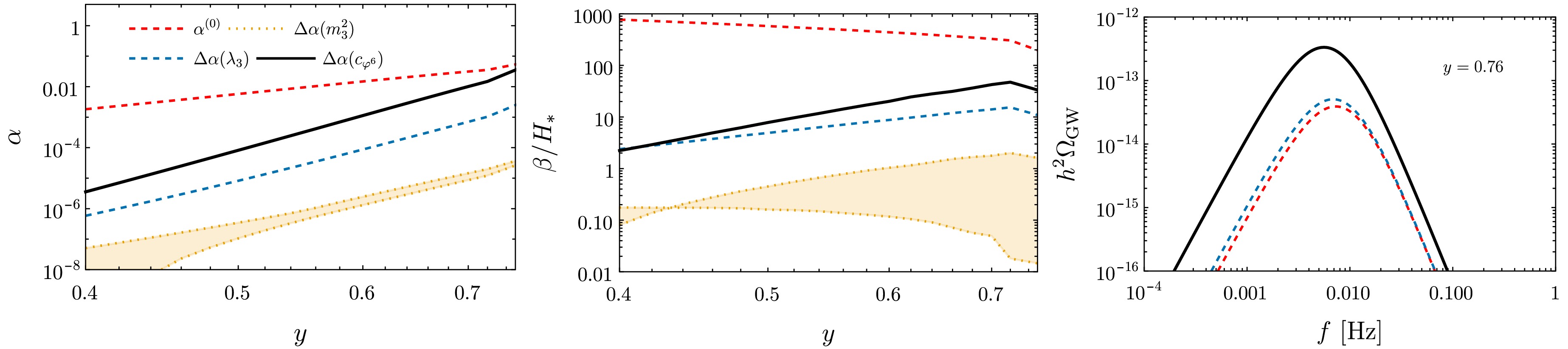
Figure 6. (Color online) Strength parameter (left), inverse duration time (middle), and corresponding GW spectrum (right) in the model of Appendix E, which extends Ref. [50] with 2-loop matching corrections and running, for a benchmark point with
$ (m^2,\kappa,\lambda) = (0.02\,{\rm{TeV}}^2, -0.04\,{\rm{TeV}}, 0.1) $ . Renormalization-scale independent holds up to order$ y^4 $ ($ y^6 $ ) for the mass (quartic coupling and higher-dimensional operators). The bands represent variations of the renormalization scale$ \mu\in [\overline{T}/2, 2\overline{T}] $ , with$ \overline{T} = \Lambda {\rm e}^{-\gamma_E} $ .Altogether, our results provide the strongest evidence to date for the central role of dimension-6 operators relative to higher-loop corrections to lower-dimensional interactions in the 3D EFT framework, particularly in the study of strong PT relevant for detection at current and future facilities. This does not necessarily imply that the high-temperature expansion is questioned, provided dimension-8-operator effects are sub-leading, which can be assessed following the methods of Ref. [50], and as we have ensured in all our results.
-
We have studied thermal-PT parameters within a model consisting of a complex scalar ϕ coupled to fermions, and in which the scalar potential exhibits two minima at zero temperature due to a
$ \phi^6 $ interaction. We have done so within the framework of dimensional reduction, computing matching corrections to the mass, quartic, and dimension-6 terms up to 3, 2, and 1 loops, respectively. This has been possible due to the unique characteristics of this model, which ensure that all 3-loop sum-integrals involved in the process are already known from studies in hot QCD.In this way, we have been able to compare, for the first time, the relative importance of the different matching corrections, which, according to standard power counting, are nominally of the same order. We have found that while 2-loop corrections to the quartic coupling compete with 1-loop corrections to
$ \varphi^6 $ , the latter generally dominate by a large margin over 3-loop corrections to the mass.To further demonstrate the relevance of higher-order-operator corrections on PT parameters, we compute α and
$ \beta/H_* $ , as well as the corresponding spectrum of GWs within the model of Appendix E, involving a real scalar singlet, a fermion, and no dimension-6 terms. We include matching corrections up to 2-loops. (Unfortunately, 3-loop sum-integrals within this model are unknown.) The results are depicted in Fig. 6. (Note that, unlike in Ref. [50], here we use$ S_3[\varphi_c]\sim 140 $ instead of$ \sim 100 $ as the nucleation criterion.) They provide even clearer evidence of the dominance of 1-loop corrections arising from dimension-6 terms. We see no reason to expect qualitatively different behavior in other models of new physics.
Figure 6. (Color online) Strength parameter (left), inverse duration time (middle), and corresponding GW spectrum (right) in the model of Appendix E, which extends Ref. [50] with 2-loop matching corrections and running, for a benchmark point with
$ (m^2,\kappa,\lambda) = $ $ (0.02\,{\rm{TeV}}^2, -0.04\,{\rm{TeV}}, 0.1) $ . Renormalization-scale independent holds up to order$ y^4 $ ($ y^6 $ ) for the mass (quartic coupling and higher-dimensional operators). The bands represent variations of the renormalization scale$ \mu\in [\overline{T}/2, 2\overline{T}] $ , with$ \overline{T} = \Lambda {\rm e}^{-\gamma_E} $ .Altogether, our results provide the strongest evidence to date for the central role of dimension-6 operators relative to higher-loop corrections to lower-dimensional interactions in the 3D EFT framework, particularly in the study of strong PT relevant for detection at current and future facilities. This does not necessarily imply that the high-temperature expansion is questioned, provided dimension-8-operator effects are sub-leading, which can be assessed following the methods of Ref. [50], and as we have ensured in all our results.
-
We are indebted to York Schröder for providing us with the analytic solution to two-loop fermionic sum-integrals. We are also grateful to Renato Fonseca for useful discussions. MC would like to thank the organisers and participants of the Portoroz 2025 workshop for valuable exchanges.
-
We are indebted to York Schröder for providing us with the analytic solution to two-loop fermionic sum-integrals. We are also grateful to Renato Fonseca for useful discussions. MC would like to thank the organisers and participants of the Portoroz 2025 workshop for valuable exchanges.
-
In what follows, we use a notation similar to that in Ref. [26] and present all our results in the
$ \overline{{\rm{MS}}} $ scheme in dimensional regularization, with$ d = 3 - 2\epsilon $ . We adopt the usual notation for sum-integrals:$ \sum {\displaystyle\int_{Q \; {\rm{or}}\; \{Q\}} } \equiv T \sum\limits_{n=-\infty}^\infty \int_q\,\,, $

(A1) where
$ Q = (Q_0, \mathbf{q}) = (m_n, \mathbf{q}) $ is a loop 4-momentum, and n labels the Matsubara modes running in the loop. The brackets denote a sum over fermionic modes —for which we have$ m_n = 2 \pi\left(n + \dfrac{1}{2}\right) T $ —, while their absence means we sum over bosonic modes —$ m_n = 2 \pi n T $ —.Furthermore,
$ \int_q \equiv \tilde{\mu}^{2\epsilon} \int \frac{d^{3-2\epsilon}q}{(2 \pi)^{3-2\epsilon}}\,, $

(A2) where
$ \tilde{\mu}^2 \equiv e^{\gamma_E} \mu^2 / (4 \pi) $ , μ being the$ \overline{{\rm{MS}}} $ scale, and$ \gamma_E $ the Euler-Mascheroni constant. -
In what follows, we use a notation similar to that in Ref. [26] and present all our results in the
$ \overline{{\rm{MS}}} $ scheme in dimensional regularization, with$ d = 3 - 2\epsilon $ . We adopt the usual notation for sum-integrals:$ \sum {\displaystyle\int_{Q \; {\rm{or}}\; \{Q\}} } \equiv T \sum\limits_{n=-\infty}^\infty \int_q\,\,, $
(A1) where
$ Q = (Q_0, \mathbf{q}) = (m_n, \mathbf{q}) $ is a loop 4-momentum, and n labels the Matsubara modes running in the loop. The brackets denote a sum over fermionic modes —for which we have$ m_n = 2 \pi\left(n + \dfrac{1}{2}\right) T $ —, while their absence means we sum over bosonic modes —$ m_n = 2 \pi n T $ —.Furthermore,
$ \int_q \equiv \tilde{\mu}^{2\epsilon} \int \frac{d^{3-2\epsilon}q}{(2 \pi)^{3-2\epsilon}}\,, $
(A2) where
$ \tilde{\mu}^2 \equiv e^{\gamma_E} \mu^2 / (4 \pi) $ , μ being the$ \overline{{\rm{MS}}} $ scale, and$ \gamma_E $ the Euler-Mascheroni constant. -
At 1-loop order, all bosonic sum-integrals, massive or massless, are known analytically. Because we expand sum-integrals in the scalar mass, we only require the massless cases, which read:
$ \hat{I}_{\alpha}^{r} \equiv \sum {\displaystyle\int_Q } \frac{Q_0^r}{Q^{2 \alpha}} = \tilde{\mu}^{2\epsilon} \frac{\left( 1 + (-1)^r \right) T}{(2 \pi T)^{2 \alpha - r - d}} \frac{\Gamma\left( \alpha - d/2 \right)}{(4 \pi)^{d/2} \Gamma\left( \alpha \right)} \zeta\left( 2 \alpha - r - d \right) \,, $

(A3) where
$ \Gamma(x) $ is the Euler gamma function, and$ \zeta(x) $ is the Riemann zeta function.In the fermionic case, when the mass is non-zero, no analytic expressions are available. In the massless case, however, one can derive a simple relation with their bosonic counterpart. Scaling the spatial loop momentum
$ q \to 2 q $ and splitting the regularized infinite sum in odd and even integers, yields$ I_{\alpha}^{r} \equiv \sum {\displaystyle\int_{\{Q\}} } \frac{Q_0^r}{Q^{2 \alpha}} = \left( 2^{2\alpha - r - d} - 1 \right) \hat{I}_{\alpha}^{r}\,. $

(A4) -
At 1-loop order, all bosonic sum-integrals, massive or massless, are known analytically. Because we expand sum-integrals in the scalar mass, we only require the massless cases, which read:
$ \hat{I}_{\alpha}^{r} \equiv \sum {\displaystyle\int_Q } \frac{Q_0^r}{Q^{2 \alpha}} = \tilde{\mu}^{2\epsilon} \frac{\left( 1 + (-1)^r \right) T}{(2 \pi T)^{2 \alpha - r - d}} \frac{\Gamma\left( \alpha - d/2 \right)}{(4 \pi)^{d/2} \Gamma\left( \alpha \right)} \zeta\left( 2 \alpha - r - d \right) \,, $
(A3) where
$ \Gamma(x) $ is the Euler gamma function, and$ \zeta(x) $ is the Riemann zeta function.In the fermionic case, when the mass is non-zero, no analytic expressions are available. In the massless case, however, one can derive a simple relation with their bosonic counterpart. Scaling the spatial loop momentum
$ q \to 2 q $ and splitting the regularized infinite sum in odd and even integers, yields$ I_{\alpha}^{r} \equiv \sum {\displaystyle\int_{\{Q\}} } \frac{Q_0^r}{Q^{2 \alpha}} = \left( 2^{2\alpha - r - d} - 1 \right) \hat{I}_{\alpha}^{r}\,. $
(A4) -
All 2-loop sum-integrals in the matching can be written in terms of two bosonic or two fermionic loop momenta. The most general 2-loop bosonic sum-integral reads:
$ \hat{I}_{\alpha \beta \gamma}^{r s} \equiv \sum {\displaystyle\int_{QR} } \frac{Q_0^r R_0^s}{Q^{2 \alpha} R^{2 \beta} (Q - R)^{2\gamma}}\,. $

(A5) To solve these, we use a recently developed algorithm [89] that fully reduces any such structure to the 1-loop masters above.
Similarly, the most general 2-loop fermionic sum-integral reads:
$ I_{\alpha \beta \gamma}^{r s} \equiv \sum {\displaystyle\int_{\{QR\}} } \frac{Q_0^r R_0^s}{Q^{2 \alpha} R^{2 \beta} ( Q - R )^{2\gamma}}\,. $

(A6) These are also known to factorize into 1-loop masters; however, in this case, no closed formula exists in the literature. Instead, these sum-integrals must be reduced on a case-by-case basis by means of symmetries induced by 4-momentum shifts and integration-by-parts relations involving spatial momenta [90].
By denoting
$ I_{\alpha \beta \gamma}^{00} \equiv I_{\alpha \beta \gamma} $ (resp.$ \hat{I}_{\alpha \beta \gamma}^{00} \equiv \hat{I}_{\alpha \beta \gamma} $ ), we present below the specific 2-loop fermionic sum-integrals we require and their corresponding reductions:$ I_{111} = 0 \,, $

(A7) $ I_{112} = \frac{1}{(d-2)(d-5)} \left( I_{220} - 2 I_{022} \right)\,, $

(A8) $ I_{121} = I_{211} = -\frac{1}{(d-2)(d-5)} I_{220}\,, $

(A9) $ I_{113}^{02} = I_{113}^{20} = \frac{(d-3)(d-4)}{2 (d-2) (d-5) (d-7)} I_{022} + \frac{d-4}{d-7} I_{013}\,, $

(A10) $ I_{131}^{02} = I_{311}^{20} = \frac{d-4}{2 (d-2) (d-7)} \left( I_{220} + \frac{d-3}{d-5} I_{022} \right)\,, $

(A11) $ I_{113}^{11} = -\frac{d-4}{2 (d-2) (d-5) (d-7)} \left( I_{220} - 2 I_{022} \right) + \frac{d-4}{d-7} I_{013}\,, $

(A12) $ I_{122}^{02} = I_{212}^{20} = -\frac{d-4}{2 (d-2) (d-7)} \left( I_{220} + \frac{4}{d-5} I_{022} \right)\,, $

(A13) $ I_{212}^{02} = I_{122}^{20} = \frac{(d-4) (d^2 - 8d + 13)}{(d-2) (d-5) (d-7)} I_{022} + \frac{1}{d-7} \left( I_{031} - I_{130} \right)\,, $

(A14) $ I_{122}^{11} = I_{212}^{11} = \frac{d-4}{(d - 2) (d - 5) (d - 7)} \left( I_{220} + \frac{d^2 - 8d + 11}{2} I_{022} \right)\,. $

(A15) Finally, these can be straightforwardly reduced to 1-loop master integrals through
$ I_{\alpha \beta 0} = I_{\alpha} I_{\beta}\,, I_{\alpha 0 \beta} = I_{0 \alpha \beta} = I_{\alpha} \hat{I}_{\beta}\,, $

(A16) where, in the second line, we have used the shifts
$ R \to R - Q $ and$ R \to -R $ . Note that if Q and R are fermionic, shifting$ R \to R - Q $ changes the nature of R to bosonic. -
All 2-loop sum-integrals in the matching can be written in terms of two bosonic or two fermionic loop momenta. The most general 2-loop bosonic sum-integral reads:
$ \hat{I}_{\alpha \beta \gamma}^{r s} \equiv \sum {\displaystyle\int_{QR} } \frac{Q_0^r R_0^s}{Q^{2 \alpha} R^{2 \beta} (Q - R)^{2\gamma}}\,. $
(A5) To solve these, we use a recently developed algorithm [89] that fully reduces any such structure to the 1-loop masters above.
Similarly, the most general 2-loop fermionic sum-integral reads:
$ I_{\alpha \beta \gamma}^{r s} \equiv \sum {\displaystyle\int_{\{QR\}} } \frac{Q_0^r R_0^s}{Q^{2 \alpha} R^{2 \beta} ( Q - R )^{2\gamma}}\,. $
(A6) These are also known to factorize into 1-loop masters; however, in this case, no closed formula exists in the literature. Instead, these sum-integrals must be reduced on a case-by-case basis by means of symmetries induced by 4-momentum shifts and integration-by-parts relations involving spatial momenta [90].
By denoting
$ I_{\alpha \beta \gamma}^{00} \equiv I_{\alpha \beta \gamma} $ (resp.$ \hat{I}_{\alpha \beta \gamma}^{00} \equiv \hat{I}_{\alpha \beta \gamma} $ ), we present below the specific 2-loop fermionic sum-integrals we require and their corresponding reductions:$ I_{111} = 0 \,, $
(A7) $ I_{112} = \frac{1}{(d-2)(d-5)} \left( I_{220} - 2 I_{022} \right)\,, $
(A8) $ I_{121} = I_{211} = -\frac{1}{(d-2)(d-5)} I_{220}\,, $
(A9) $ I_{113}^{02} = I_{113}^{20} = \frac{(d-3)(d-4)}{2 (d-2) (d-5) (d-7)} I_{022} + \frac{d-4}{d-7} I_{013}\,, $
(A10) $ I_{131}^{02} = I_{311}^{20} = \frac{d-4}{2 (d-2) (d-7)} \left( I_{220} + \frac{d-3}{d-5} I_{022} \right)\,, $
(A11) $ I_{113}^{11} = -\frac{d-4}{2 (d-2) (d-5) (d-7)} \left( I_{220} - 2 I_{022} \right) + \frac{d-4}{d-7} I_{013}\,, $
(A12) $ I_{122}^{02} = I_{212}^{20} = -\frac{d-4}{2 (d-2) (d-7)} \left( I_{220} + \frac{4}{d-5} I_{022} \right)\,, $
(A13) $ I_{212}^{02} = I_{122}^{20} = \frac{(d-4) (d^2 - 8d + 13)}{(d-2) (d-5) (d-7)} I_{022} + \frac{1}{d-7} \left( I_{031} - I_{130} \right)\,, $
(A14) $ I_{122}^{11} = I_{212}^{11} = \frac{d-4}{(d - 2) (d - 5) (d - 7)} \left( I_{220} + \frac{d^2 - 8d + 11}{2} I_{022} \right)\,. $
(A15) Finally, these can be straightforwardly reduced to 1-loop master integrals through
$ I_{\alpha \beta 0} = I_{\alpha} I_{\beta}\,, I_{\alpha 0 \beta} = I_{0 \alpha \beta} = I_{\alpha} \hat{I}_{\beta}\,, $
(A16) where, in the second line, we have used the shifts
$ R \to R - Q $ and$ R \to -R $ . Note that if Q and R are fermionic, shifting$ R \to R - Q $ changes the nature of R to bosonic. -
The evaluation of general 3-loop vacuum sum-integrals (bosonic, fermionic, or mixed) is currently an open problem. However, for our present purpose, all cases have been conveniently solved in the context of hot QCD.
The first subset that we find are trivial products of 1-loop masters:
$ \sum {\displaystyle\int_{QRH} } \frac{1}{Q^{2 \alpha} R^{2 \beta} H^{2 \gamma}} = \hat{I}_{\alpha} \hat{I}_{\beta} \hat{I}_{\gamma} \,. $

(A17) Others factorize into products of 1-loop masters and 2-loop sum-integrals, which we know how to further reduce to 1-loop masters. An example would be:
$ \sum {\displaystyle\int_{QRH} } \frac{1}{Q^{2 \alpha} R^{2 \beta} H^{2 \gamma} (R-H)^{2 \delta}} = \hat{I}_{\alpha} \hat{I}_{\beta \gamma \delta}\,. $

(A18) Finally, we also find non-trivial cases that are known analytically in the literature. In Eq. (25) of Ref. [91], we find
$ \begin{split}& \sum {\displaystyle\int_{QRH} } \frac{1}{Q^4 H^2 (Q-R)^2 (R-H)^2}\\& \qquad = \tilde{\mu}^{6 \epsilon} \left\{ \frac{T^2 (4\pi T^2)^{-3\epsilon}}{8(4\pi)^4\epsilon^2} \left[ 1+b_{21}\epsilon +b_{22}\epsilon^2 + {\cal{O}}(\epsilon^3) \right] \right\}\\ & \qquad b_{21}= \frac{17}{6} + \gamma_E + 2 \frac{\zeta'(-1)}{\zeta(-1)} \\& \qquad b_{22} = \frac{131}{12} +\frac{31\pi^2}{36} +8\log 2\pi -\frac{9\gamma_E}{2} \\ & \qquad - \frac{15\gamma_E^2}{2} + (5+2\gamma_E) \frac{\zeta'(-1)}{\zeta(-1)} + 2 \frac{\zeta''(-1)}{\zeta(-1)} - 16 \gamma_1 \\ & \qquad + \frac{4\zeta(3)}{9} + C_{b} \,, \end{split} $

(A19) where
$ \gamma_1 $ is one of the Stieltjes constants:$ \zeta(1+\epsilon) = 1/\epsilon + \displaystyle\sum_{n=0}^\infty (-1)^n \gamma_n \epsilon^n /n! $ ; and the constant$ C_{b} = -0.145652981107 (4) $ is a sum of several dimensionless integrals that have been evaluated numerically. We have manually added the scale factor according to our definition of the integral measure.Additionally, in Eq. (36) of Ref. [92], we find
$ \begin{split} &\sum {\displaystyle\int_{QRH} } \frac{1}{Q^2 R^2 H^2 (Q+R+H)^2} \\& \qquad = \frac{1}{(4 \pi)^2} \left( \frac{T^2}{12} \right)^2 \bigg[\frac{6}{\epsilon} + 36 \log\frac{\mu}{4 \pi T} - 12 \frac{\zeta'(-3)}{\zeta(-3)} \\ & \qquad + 48 \frac{\zeta'(-1)}{\zeta(-1)} + \frac{182}{5} \bigg] + {\cal{O}}(\epsilon)\,, \end{split} $

(A20) which assumes the same integral measure we use. Note that the result is expressed in terms of the
$ \overline{{\rm{MS}}} $ scale μ, and not in terms of$ \tilde{\mu} $ .Finally, from Eq. (15) of Ref. [93], we have
$ \begin{split} &\sum {\displaystyle\int_{QRH} } \frac{1}{Q^2 R^2 H^2 (Q-R)^2 (Q-H)^2} \\ & \qquad = \tilde{\mu}^{6 \epsilon} \left\{-\frac{1}{4} \frac{T^2}{(4 \pi)^4} \frac{(4 \pi e^{\gamma_E} T^2)^{-3 \epsilon}}{\epsilon^2} \left[ 1 + v_1 \epsilon + v_2 \epsilon^2 + {\cal{O}}(\epsilon^3)\right] \right\}\,; \\ & \qquad v_1 = \frac{4}{3} + 4 \gamma_E + 2 \frac{\zeta'(-1)}{\zeta(-1)} \,, v_2 = \frac{1}{3} \left[ 46 - 16 \gamma_E^2 \right. \\& \qquad+ \frac{45 \pi^2}{4} + 24 \log^2 2 \pi - 104 \gamma_1 - 8 \gamma_E -24 \gamma_E \log 2 \pi \\ & \left. \qquad+ 16 \gamma_E \frac{\zeta'(-1)}{\zeta(-1)} + 24 \frac{\zeta'(-1)}{\zeta(-1)} + 2 \frac{\zeta''(-1)}{\zeta(-1)} \right] + C_{s} \,, \end{split} $

(A21) where the constant
$ C_{s} = - 38.5309 $ is a sum of several dimensionless integrals that have been evaluated numerically. -
The evaluation of general 3-loop vacuum sum-integrals (bosonic, fermionic, or mixed) is currently an open problem. However, for our present purpose, all cases have been conveniently solved in the context of hot QCD.
The first subset that we find are trivial products of 1-loop masters:
$ \sum {\displaystyle\int_{QRH} } \frac{1}{Q^{2 \alpha} R^{2 \beta} H^{2 \gamma}} = \hat{I}_{\alpha} \hat{I}_{\beta} \hat{I}_{\gamma} \,. $
(A17) Others factorize into products of 1-loop masters and 2-loop sum-integrals, which we know how to further reduce to 1-loop masters. An example would be:
$ \sum {\displaystyle\int_{QRH} } \frac{1}{Q^{2 \alpha} R^{2 \beta} H^{2 \gamma} (R-H)^{2 \delta}} = \hat{I}_{\alpha} \hat{I}_{\beta \gamma \delta}\,. $
(A18) Finally, we also find non-trivial cases that are known analytically in the literature. In Eq. (25) of Ref. [91], we find
$ \begin{split}& \sum {\displaystyle\int_{QRH} } \frac{1}{Q^4 H^2 (Q-R)^2 (R-H)^2}\\& \qquad = \tilde{\mu}^{6 \epsilon} \left\{ \frac{T^2 (4\pi T^2)^{-3\epsilon}}{8(4\pi)^4\epsilon^2} \left[ 1+b_{21}\epsilon +b_{22}\epsilon^2 + {\cal{O}}(\epsilon^3) \right] \right\}\\ & \qquad b_{21}= \frac{17}{6} + \gamma_E + 2 \frac{\zeta'(-1)}{\zeta(-1)} \\& \qquad b_{22} = \frac{131}{12} +\frac{31\pi^2}{36} +8\log 2\pi -\frac{9\gamma_E}{2} \\ & \qquad - \frac{15\gamma_E^2}{2} + (5+2\gamma_E) \frac{\zeta'(-1)}{\zeta(-1)} + 2 \frac{\zeta''(-1)}{\zeta(-1)} - 16 \gamma_1 \\ & \qquad + \frac{4\zeta(3)}{9} + C_{b} \,, \end{split} $
(A19) where
$ \gamma_1 $ is one of the Stieltjes constants:$ \zeta(1+\epsilon) = 1/\epsilon + \displaystyle\sum_{n=0}^\infty (-1)^n \gamma_n \epsilon^n /n! $ ; and the constant$ C_{b} = -0.145652981107 (4) $ is a sum of several dimensionless integrals that have been evaluated numerically. We have manually added the scale factor according to our definition of the integral measure.Additionally, in Eq. (36) of Ref. [92], we find
$ \begin{split} &\sum {\displaystyle\int_{QRH} } \frac{1}{Q^2 R^2 H^2 (Q+R+H)^2} \\& \qquad = \frac{1}{(4 \pi)^2} \left( \frac{T^2}{12} \right)^2 \bigg[\frac{6}{\epsilon} + 36 \log\frac{\mu}{4 \pi T} - 12 \frac{\zeta'(-3)}{\zeta(-3)} \\ & \qquad + 48 \frac{\zeta'(-1)}{\zeta(-1)} + \frac{182}{5} \bigg] + {\cal{O}}(\epsilon)\,, \end{split} $
(A20) which assumes the same integral measure we use. Note that the result is expressed in terms of the
$ \overline{{\rm{MS}}} $ scale μ, and not in terms of$ \tilde{\mu} $ .Finally, from Eq. (15) of Ref. [93], we have
$ \begin{split} &\sum {\displaystyle\int_{QRH} } \frac{1}{Q^2 R^2 H^2 (Q-R)^2 (Q-H)^2} \\ & \qquad = \tilde{\mu}^{6 \epsilon} \left\{-\frac{1}{4} \frac{T^2}{(4 \pi)^4} \frac{(4 \pi e^{\gamma_E} T^2)^{-3 \epsilon}}{\epsilon^2} \left[ 1 + v_1 \epsilon + v_2 \epsilon^2 + {\cal{O}}(\epsilon^3)\right] \right\}\,; \\ & \qquad v_1 = \frac{4}{3} + 4 \gamma_E + 2 \frac{\zeta'(-1)}{\zeta(-1)} \,, v_2 = \frac{1}{3} \left[ 46 - 16 \gamma_E^2 \right. \\& \qquad+ \frac{45 \pi^2}{4} + 24 \log^2 2 \pi - 104 \gamma_1 - 8 \gamma_E -24 \gamma_E \log 2 \pi \\ & \left. \qquad+ 16 \gamma_E \frac{\zeta'(-1)}{\zeta(-1)} + 24 \frac{\zeta'(-1)}{\zeta(-1)} + 2 \frac{\zeta''(-1)}{\zeta(-1)} \right] + C_{s} \,, \end{split} $
(A21) where the constant
$ C_{s} = - 38.5309 $ is a sum of several dimensionless integrals that have been evaluated numerically. -
We start describing the CT Lagrangian in the 4D theory:
$ \begin{split} {\cal{L}}_{4, \rm ct} &= \delta K_\phi \partial_\mu\phi^\dagger \partial^\mu\phi - \delta m^2 \phi^\dagger\phi - \delta\lambda(\phi^\dagger\phi)^2 - \frac{\delta c_{\phi^6}}{\Lambda^2}(\phi^\dagger\phi)^3\,, \\ &\hphantom= + {\rm i} \delta K_\psi \left( \overline{\psi_L}\not{\partial}\psi_L + {\rm i} \overline{\psi_R}\not{\partial}\psi_R \right) - \delta y (\phi \overline{\psi_L}\psi_R+\text{h.c.})\,, \end{split} $

(B1) as well as the counterpart in the 3D EFT:
$ \begin{split} {\cal{L}}_{\text{EFT}, \rm ct} &= \delta Z_\varphi (\partial_{\mu} \varphi)^{\dagger} (\partial^{\mu} \varphi) + \delta m_3^2 \varphi^{\dagger} \varphi + \delta\lambda_3 (\varphi^{\dagger} \varphi)^2 + \delta c_{\varphi^6}(\varphi^{\dagger} \varphi)^3 \\ &\hphantom= + \delta c^{(1)}_{\partial^2 \varphi^4} (\varphi^{\dagger} \varphi) (\partial_{\mu} \varphi^{\dagger} \partial^{\mu} \varphi) + \delta r^{(2)}_{\partial^2 \varphi^4} \left[(\varphi^{\dagger} \varphi) (\partial^2 \varphi^{\dagger} \varphi) + \text{h.c.}\right] \\ &\hphantom= + \delta r^{(3)}_{\partial^2 \varphi^4} \left[i(\varphi^{\dagger} \varphi) (\partial^2 \varphi^{\dagger} \varphi) + \text{h.c.}\right] + \delta r_{\partial^4 \varphi^2} (\varphi^{\dagger} \partial^4 \varphi)\,. \end{split} $

(B2) As a clarifying example, we first explicitly derive
$ \delta \lambda $ and then$ \delta \lambda_3 $ to order$ \lambda^3 $ . The relevant diagrams are shown in Fig. A1, among which only the sunset diagram, that is, the 8th diagram in Fig. A1, contributes to$ \delta \lambda_3 $ . We work in the$ \rm \overline{MS} $ -scheme in dimensional regularization.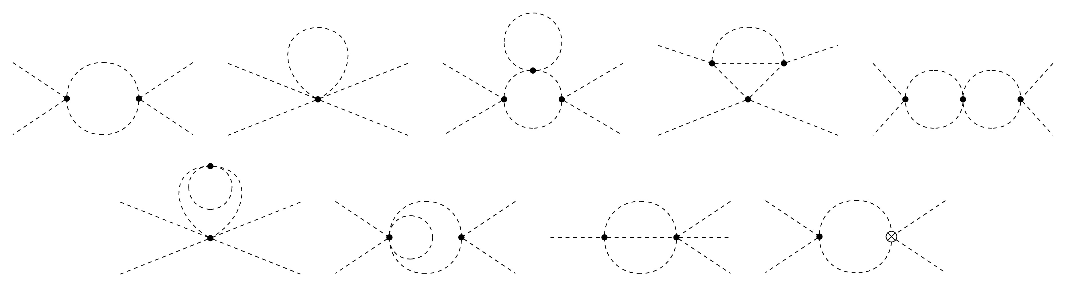
Figure A1. Relevant 1-loop and 2-loop diagrams for the running of the 4-point functions in the 4D theory and the 3D EFT. The cross with one circle denotes the 1-loop CT.
In the 4D theory, we split the 4-point function with the scalar in the external legs in loop orders as
$ \Gamma_{\phi\phi\phi\phi} = \Gamma_{\phi\phi\phi\phi}^{(0)} + \Gamma_{\phi\phi\phi\phi}^{(1)} + \Gamma_{\phi\phi\phi\phi}^{(2)} \,, $

(B3) and we present each piece separately, after simplifying the traces of gamma matrices and removing higher order terms. We do the same for the CT correlators, which we denote
$ \Gamma_{\phi\phi\phi\phi, \rm ct}^{(\ell)} $ . For convenience, let us also define a pole-subtracting operator$ {\cal{K}} $ with the property that$ {\cal{K}}\left( a_0 + \sum\limits_{k=1}^n \frac{a_k}{\epsilon^k} \right) = \sum\limits_{k=1}^n \frac{a_k}{\epsilon^k}\,, $

(B4) with
$ a_k \in \mathbb{C}, k=0, 1, 2, \dots $ being$ \epsilon $ -independent.Since the tree-level part is not divergent, let us start with the 1-loop, which reads:
$ \Gamma_{\phi\phi\phi\phi}^{(1)} = 40 \lambda^2 \int_q \frac{1}{(q^2 - m^2)^2} + 36 \frac{c_{\phi^6}}{\Lambda^2} \int_q \frac{1}{q^2 - m^2} \,, $

(B5) where we use the same notation as in Eq. (A2) but in
$ d=4-2\epsilon $ .The evaluation of these 1-loop integrals in dimensional regularization is straightforward, and it can be found in any standard QFT textbook (see e.g., Appendix B in Ref. [94]). The result is:
$ {\cal{K}} \left(\Gamma_{\phi\phi\phi\phi}^{(1)}\right) = \frac{\rm i}{4 \pi^2 \epsilon} \left( 10 \lambda^2 + 9 m^2 \frac{c_{\phi^6}}{\Lambda^2} \right)\,. $

(B6) The corresponding CT diagram is
$ \Gamma_{\phi\phi\phi\phi, \rm ct}^{(1)} = -4 {\rm i} \delta \lambda^{(1)}\,. $

(B7) Therefore, by definition,
$ \delta\lambda^{(1)} = \frac{1}{8 \pi^2} \left( 5 \lambda^2 + \frac{9}{2} m^2 \frac{c_{\phi^6}}{\Lambda^2} \right)\,. $

(B8) At 2-loop level, we have
$ \begin{split} \Gamma_{\phi\phi\phi\phi}^{(2)} =& 288 i \lambda \frac{c_{\phi^6}}{\Lambda^2} \int_{q, k} \frac{1}{(q^2-m^2)(k^2-m^2)[(q+k)^2-m^2]} \\ &+ 144 i \lambda \frac{c_{\phi^6}}{\Lambda^2} \int_{q, k} \frac{1}{(q^2-m^2)(k^2-m^2)^2} \\&+ 720 i \lambda \frac{c_{\phi^6}}{\Lambda^2} \int_{q, k} \frac{1}{(q^2-m^2)^2 (k^2-m^2)} \\ &+ 512 i \lambda^3 \int_{q, k} \frac{1}{(q^2-m^2)(k^2-m^2)[(q+k)^2-m^2]^2} \\ &+ 144 i \lambda^3 \int_{q, k} \frac{1}{(q^2-m^2)^2 (k^2-m^2)^2} \\&+ 320 i \lambda^3 \int_{q, k} \frac{1}{(q^2-m^2)^3 (k^2-m^2)}\,. \end{split} $

(B9) Using the known formulae for 2-loop tadpole integrals in Ref. [95], we find that the divergent part is, neglecting higher orders,
$ {\cal{K}}\left(\Gamma_{\phi\phi\phi\phi}^{(2)}\right) = \frac{{\rm i} \lambda^3}{16 \pi^4} \left[ \left( - 6 - 100 \log \frac{\mu}{m} \right) \frac{1}{\epsilon} - \frac{25}{\epsilon^2} \right]\,. $

(B10) Now, for simplicity, let us assume that we already know the rest of the 1-loop CTs, which can be easily obtained following the method used for
$ \delta\lambda^{(1)} $ . Although they do not appear explicitly in this example, it is important to note that loops involving massless fermions must be treated with care, as they can induce mixing between UV and IR divergences. To avoid this, we introduce a spurious mass$ m_f $ that we take to zero once all integrals have been evaluated.From the CT diagrams, the only terms of order
$ {\cal{O}}(\lambda^3) $ are$ \Gamma_{\phi\phi\phi\phi, \rm ct}^{(2)} = 80 \delta\lambda^{(1)} \lambda \int_q \frac{1}{(q^2-m^2)^2} - 4 {\rm i} \delta \lambda^{(2)}\,, $

(B11) which yields
$ {\cal{K}} \left(\Gamma_{\phi\phi\phi\phi, \rm ct}^{(2)}\right) = \frac{{\rm i} \lambda^3}{16 \pi^4} \left[ \left(-10 + 100 \log \frac{\mu}{m} \right) \frac{1}{\epsilon} + \frac{50}{\epsilon^2} \right] - 4 {\rm i} \delta \lambda^{(2)} \,. $

(B12) Summing Eqs. (B11) and (B12), we find
$ \delta\lambda^{(2)} = \frac{\lambda^3}{64 \pi^4} \left( - \frac{16}{\epsilon} + \frac{25}{\epsilon^2} \right)\,. $

(B13) Thus, we recover the CT shown in Eq. (13) in the main text.
For the computation of
$ \delta \lambda_3 $ , the process is analogous but simpler. We split the 4-point function in loop orders as$ \Gamma_{\varphi\varphi\varphi\varphi} = \Gamma_{\varphi\varphi\varphi\varphi}^{(0)} + \Gamma_{\varphi\varphi\varphi\varphi}^{(1)} + \Gamma_{\varphi\varphi\varphi\varphi}^{(2)} \,. $

(B14) and present all results in Euclidean space.
We know that
$ \Gamma_{\varphi\varphi\varphi\varphi}^{(1)} $ cannot be divergent, as there are no divergent tadpole integrals at 1-loop order in$ d=3 $ . Therefore,$ \delta \lambda_3^{(1)} = 0\,. $

(B15) At 2-loop order, we also know that the only divergent tadpole integral is the one associated to the sunset diagram. Therefore, focusing on this type only, we have
$ \Gamma_{\varphi\varphi\varphi\varphi}^{(2)} = - 288 \lambda_3 c_{\varphi^6} \int_{q, r} \frac{1}{(q^2 + m_3^2)(r^2 + m_3^2)[(q+r)^2 + m_3^2]} + \dots $

(B16) where the ellipses include all other non-divergent contributions. Again, using the known formulae for massive 2-loop integrals, we obtain:
$ {\cal{K}} \left(\Gamma_{\varphi\varphi\varphi\varphi}^{(2)} \right) = \frac{9}{2 \pi^2} \lambda_3 c_{\varphi^6}\,. $

(B17) Since there are no 1-loop CTs, we must only compute the tree-level insertion of 2-loop CTs, which yields:
$ \Gamma_{\varphi\varphi\varphi\varphi, \rm ct}^{(2)} = - 4 \delta \lambda_3^{(2)} + \dots $

(B18) Therefore, we obtain:
$ \delta \lambda_3^{(2)} = \frac{9}{8 \pi^2} \lambda_3 c_{\varphi^6}\,, $

(B19) as shown in Eq. (17) in the main text.
-
We start describing the CT Lagrangian in the 4D theory:
$ \begin{split} {\cal{L}}_{4, \rm ct} &= \delta K_\phi \partial_\mu\phi^\dagger \partial^\mu\phi - \delta m^2 \phi^\dagger\phi - \delta\lambda(\phi^\dagger\phi)^2 - \frac{\delta c_{\phi^6}}{\Lambda^2}(\phi^\dagger\phi)^3\,, \\ &\hphantom= + {\rm i} \delta K_\psi \left( \overline{\psi_L}\not{\partial}\psi_L + {\rm i} \overline{\psi_R}\not{\partial}\psi_R \right) - \delta y (\phi \overline{\psi_L}\psi_R+\text{h.c.})\,, \end{split} $
(B1) as well as the counterpart in the 3D EFT:
$ \begin{split} {\cal{L}}_{\text{EFT}, \rm ct} &= \delta Z_\varphi (\partial_{\mu} \varphi)^{\dagger} (\partial^{\mu} \varphi) + \delta m_3^2 \varphi^{\dagger} \varphi + \delta\lambda_3 (\varphi^{\dagger} \varphi)^2 + \delta c_{\varphi^6}(\varphi^{\dagger} \varphi)^3 \\ &\hphantom= + \delta c^{(1)}_{\partial^2 \varphi^4} (\varphi^{\dagger} \varphi) (\partial_{\mu} \varphi^{\dagger} \partial^{\mu} \varphi) + \delta r^{(2)}_{\partial^2 \varphi^4} \left[(\varphi^{\dagger} \varphi) (\partial^2 \varphi^{\dagger} \varphi) + \text{h.c.}\right] \\ &\hphantom= + \delta r^{(3)}_{\partial^2 \varphi^4} \left[i(\varphi^{\dagger} \varphi) (\partial^2 \varphi^{\dagger} \varphi) + \text{h.c.}\right] + \delta r_{\partial^4 \varphi^2} (\varphi^{\dagger} \partial^4 \varphi)\,. \end{split} $
(B2) As a clarifying example, we first explicitly derive
$ \delta \lambda $ and then$ \delta \lambda_3 $ to order$ \lambda^3 $ . The relevant diagrams are shown in Fig. A1, among which only the sunset diagram, that is, the 8th diagram in Fig. A1, contributes to$ \delta \lambda_3 $ . We work in the$ \rm \overline{MS} $ -scheme in dimensional regularization.
Figure A1. Relevant 1-loop and 2-loop diagrams for the running of the 4-point functions in the 4D theory and the 3D EFT. The cross with one circle denotes the 1-loop CT.
In the 4D theory, we split the 4-point function with the scalar in the external legs in loop orders as
$ \Gamma_{\phi\phi\phi\phi} = \Gamma_{\phi\phi\phi\phi}^{(0)} + \Gamma_{\phi\phi\phi\phi}^{(1)} + \Gamma_{\phi\phi\phi\phi}^{(2)} \,, $
(B3) and we present each piece separately, after simplifying the traces of gamma matrices and removing higher order terms. We do the same for the CT correlators, which we denote
$ \Gamma_{\phi\phi\phi\phi, \rm ct}^{(\ell)} $ . For convenience, let us also define a pole-subtracting operator$ {\cal{K}} $ with the property that$ {\cal{K}}\left( a_0 + \sum\limits_{k=1}^n \frac{a_k}{\epsilon^k} \right) = \sum\limits_{k=1}^n \frac{a_k}{\epsilon^k}\,, $
(B4) with
$ a_k \in \mathbb{C}, k=0, 1, 2, \dots $ being$ \epsilon $ -independent.Since the tree-level part is not divergent, let us start with the 1-loop, which reads:
$ \Gamma_{\phi\phi\phi\phi}^{(1)} = 40 \lambda^2 \int_q \frac{1}{(q^2 - m^2)^2} + 36 \frac{c_{\phi^6}}{\Lambda^2} \int_q \frac{1}{q^2 - m^2} \,, $
(B5) where we use the same notation as in Eq. (A2) but in
$ d=4-2\epsilon $ .The evaluation of these 1-loop integrals in dimensional regularization is straightforward, and it can be found in any standard QFT textbook (see e.g., Appendix B in Ref. [94]). The result is:
$ {\cal{K}} \left(\Gamma_{\phi\phi\phi\phi}^{(1)}\right) = \frac{\rm i}{4 \pi^2 \epsilon} \left( 10 \lambda^2 + 9 m^2 \frac{c_{\phi^6}}{\Lambda^2} \right)\,. $
(B6) The corresponding CT diagram is
$ \Gamma_{\phi\phi\phi\phi, \rm ct}^{(1)} = -4 {\rm i} \delta \lambda^{(1)}\,. $
(B7) Therefore, by definition,
$ \delta\lambda^{(1)} = \frac{1}{8 \pi^2} \left( 5 \lambda^2 + \frac{9}{2} m^2 \frac{c_{\phi^6}}{\Lambda^2} \right)\,. $
(B8) At 2-loop level, we have
$ \begin{split} \Gamma_{\phi\phi\phi\phi}^{(2)} =& 288 i \lambda \frac{c_{\phi^6}}{\Lambda^2} \int_{q, k} \frac{1}{(q^2-m^2)(k^2-m^2)[(q+k)^2-m^2]} \\ &+ 144 i \lambda \frac{c_{\phi^6}}{\Lambda^2} \int_{q, k} \frac{1}{(q^2-m^2)(k^2-m^2)^2} \\&+ 720 i \lambda \frac{c_{\phi^6}}{\Lambda^2} \int_{q, k} \frac{1}{(q^2-m^2)^2 (k^2-m^2)} \\ &+ 512 i \lambda^3 \int_{q, k} \frac{1}{(q^2-m^2)(k^2-m^2)[(q+k)^2-m^2]^2} \\ &+ 144 i \lambda^3 \int_{q, k} \frac{1}{(q^2-m^2)^2 (k^2-m^2)^2} \\&+ 320 i \lambda^3 \int_{q, k} \frac{1}{(q^2-m^2)^3 (k^2-m^2)}\,. \end{split} $
(B9) Using the known formulae for 2-loop tadpole integrals in Ref. [95], we find that the divergent part is, neglecting higher orders,
$ {\cal{K}}\left(\Gamma_{\phi\phi\phi\phi}^{(2)}\right) = \frac{{\rm i} \lambda^3}{16 \pi^4} \left[ \left( - 6 - 100 \log \frac{\mu}{m} \right) \frac{1}{\epsilon} - \frac{25}{\epsilon^2} \right]\,. $
(B10) Now, for simplicity, let us assume that we already know the rest of the 1-loop CTs, which can be easily obtained following the method used for
$ \delta\lambda^{(1)} $ . Although they do not appear explicitly in this example, it is important to note that loops involving massless fermions must be treated with care, as they can induce mixing between UV and IR divergences. To avoid this, we introduce a spurious mass$ m_f $ that we take to zero once all integrals have been evaluated.From the CT diagrams, the only terms of order
$ {\cal{O}}(\lambda^3) $ are$ \Gamma_{\phi\phi\phi\phi, \rm ct}^{(2)} = 80 \delta\lambda^{(1)} \lambda \int_q \frac{1}{(q^2-m^2)^2} - 4 {\rm i} \delta \lambda^{(2)}\,, $
(B11) which yields
$ {\cal{K}} \left(\Gamma_{\phi\phi\phi\phi, \rm ct}^{(2)}\right) = \frac{{\rm i} \lambda^3}{16 \pi^4} \left[ \left(-10 + 100 \log \frac{\mu}{m} \right) \frac{1}{\epsilon} + \frac{50}{\epsilon^2} \right] - 4 {\rm i} \delta \lambda^{(2)} \,. $
(B12) Summing Eqs. (B11) and (B12), we find
$ \delta\lambda^{(2)} = \frac{\lambda^3}{64 \pi^4} \left( - \frac{16}{\epsilon} + \frac{25}{\epsilon^2} \right)\,. $
(B13) Thus, we recover the CT shown in Eq. (13) in the main text.
For the computation of
$ \delta \lambda_3 $ , the process is analogous but simpler. We split the 4-point function in loop orders as$ \Gamma_{\varphi\varphi\varphi\varphi} = \Gamma_{\varphi\varphi\varphi\varphi}^{(0)} + \Gamma_{\varphi\varphi\varphi\varphi}^{(1)} + \Gamma_{\varphi\varphi\varphi\varphi}^{(2)} \,. $
(B14) and present all results in Euclidean space.
We know that
$ \Gamma_{\varphi\varphi\varphi\varphi}^{(1)} $ cannot be divergent, as there are no divergent tadpole integrals at 1-loop order in$ d=3 $ . Therefore,$ \delta \lambda_3^{(1)} = 0\,. $
(B15) At 2-loop order, we also know that the only divergent tadpole integral is the one associated to the sunset diagram. Therefore, focusing on this type only, we have
$ \Gamma_{\varphi\varphi\varphi\varphi}^{(2)} = - 288 \lambda_3 c_{\varphi^6} \int_{q, r} \frac{1}{(q^2 + m_3^2)(r^2 + m_3^2)[(q+r)^2 + m_3^2]} + \dots $
(B16) where the ellipses include all other non-divergent contributions. Again, using the known formulae for massive 2-loop integrals, we obtain:
$ {\cal{K}} \left(\Gamma_{\varphi\varphi\varphi\varphi}^{(2)} \right) = \frac{9}{2 \pi^2} \lambda_3 c_{\varphi^6}\,. $
(B17) Since there are no 1-loop CTs, we must only compute the tree-level insertion of 2-loop CTs, which yields:
$ \Gamma_{\varphi\varphi\varphi\varphi, \rm ct}^{(2)} = - 4 \delta \lambda_3^{(2)} + \dots $
(B18) Therefore, we obtain:
$ \delta \lambda_3^{(2)} = \frac{9}{8 \pi^2} \lambda_3 c_{\varphi^6}\,, $
(B19) as shown in Eq. (17) in the main text.
-
As stated in the main text, we have the following power counting in the 4D theory:
$ y \sim \frac{m^2}{T^2} \sim \frac{|\mathbf{p}|^2}{T^2} \sim \lambda\,,\quad \frac{c_{\phi^6}}{\Lambda^2} \sim \lambda^2\,. $

(C1) To perform the hard region expansion of 4D correlators, we expand in powers of
$ |\mathbf{p}|^2/T^2 $ and$ m^2/T^2 $ by iterating the following identity:$ \frac{1}{(Q+P)^2 + m^2} = \frac{1}{Q^2 + m^2} \left[ 1 - \frac{P^2 + 2 (Q \cdot P) + m^2}{(Q+P)^2 + m^2} \right] \,, $

(C2) and Taylor-expanding in
$ m^2/Q^2 $ up to the needed order in λ.We use the following tensor reduction formulae to simplify different tensor structures to scalar integrals:
$ \begin{split} q_i r_j =& \frac{\mathbf{q} \cdot \mathbf{r}}{d} \delta_{ij} \,, \\ q_i r_j r_k r_l =& \frac{|\mathbf{r}|^2 \left(\mathbf{q} \cdot \mathbf{r} \right)}{d^2 + 2 d} \left( \delta_{ij} \delta_{kl} + \delta_{ik} \delta_{jl} + \delta_{il} \delta_{jk} \right) \,, \\ q_i q_j r_k r_l =& \frac{\left( \delta_{ik} \delta_{jl} + \delta_{il} \delta_{jk}\right) \left[ d \left( \mathbf{q} \cdot \mathbf{r} \right)^2 - |\mathbf{q}|^2 |\mathbf{r}|^2\right]+ \delta_{ij} \delta_{kl} \left[(d+1) |\mathbf{q}|^2 |\mathbf{r}|^2 - 2 \left( \mathbf{q} \cdot \mathbf{r} \right)^2 \right]}{d (d-1) (d+2)}\,, \end{split} $

(C3) where
$ q_i $ and$ r_i $ are spatial 3-momenta. The same reductions in the case of one single independent loop momentum can be read from the ones above by simply setting$ q_i = r_i $ .Finally, we employ specific linear shifts of loop momenta together with algebraic identities to express all scalar vacuum sum-integrals in terms of master sum-integrals, which remain to be evaluated (see Appendix A). As an explicit example of the procedure above, we detail how to obtain the matching equation for the kinetic term of the scalar in the EFT up to order
$ \lambda^3 $ , that is, the result in Eq. (23). The relevant diagrams for the 2-point function are shown in Figs. A2 and A3.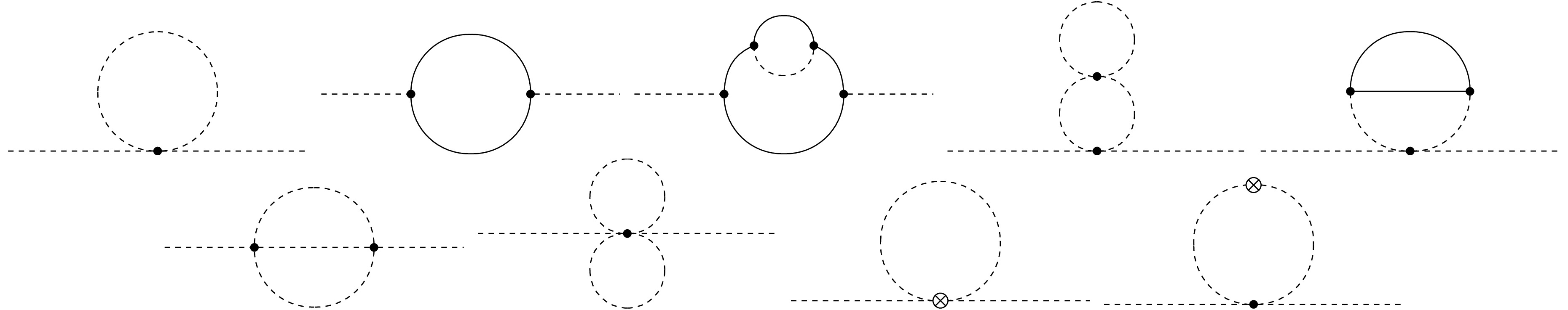
Figure A2. 1-loop and 2-loop diagrams for the 2-point function. The crosses with one circle denote the 1-loop CTs.
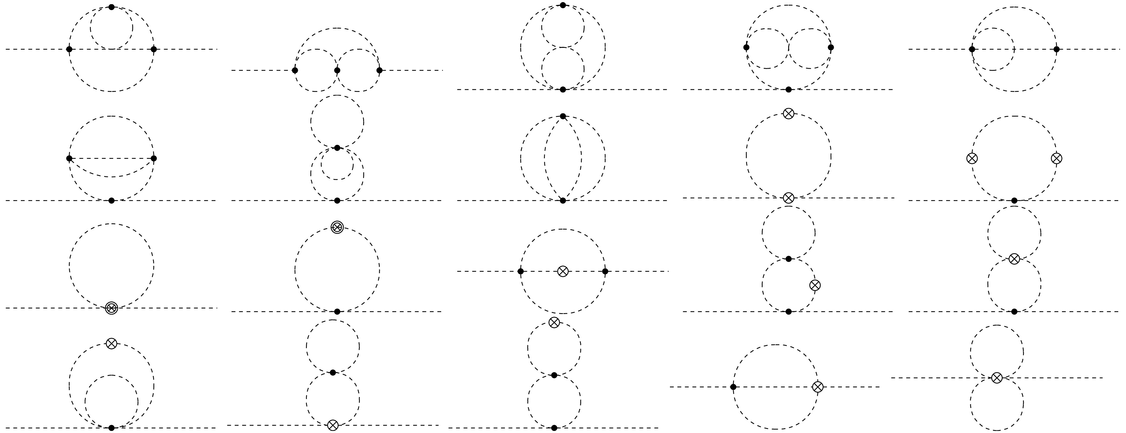
Figure A3. 3-loop diagrams for the 2-point function. The crosses with one circle denote the 1-loop CTs and the crosses with two circles denote the 2-loop CTs.
Let us first note that while the 3-loop diagrams represented in Fig. A3 contribute to the matching of the effective mass, they do not contribute to the kinetic term up to order
$ \lambda^3 $ . This is because the vertex prefactor of all 3-loop diagrams already add up to this order; hence, their expansion in external momentum up to$ |\mathbf{p}|^2 $ is at least$ {\cal{O}}(\lambda^4) $ according to our power counting.We split the 2-point function with the scalar zero mode in the external legs in loop orders as
$ \Gamma_{\phi_0 \phi_0} \equiv \Gamma_{\phi_0 \phi_0}^{(0)} + \Gamma_{\phi_0 \phi_0}^{(1)} + \Gamma_{\phi_0 \phi_0}^{(2)}\,, $

(C4) and we present each piece separately in Euclidean space and after simplifying the traces of gamma matrices in fermionic sum-integrals.
The tree-level trivially reads:
$ \Gamma_{\phi_0 \phi_0}^{(0)} = -P^2 - m^2 \,. $

(C5) The 1-loop piece, which corresponds to the first two diagrams in Fig. A2 together with tree-level insertions of 1-loop CTs, is
$ \begin{split} \Gamma_{\phi_0 \phi_0}^{(1)} = &- 4 \lambda \sum {\displaystyle\int_Q } \frac{1}{Q^2 + m^2} \\&+ 6 y^2 \sum {\displaystyle\int_{\{Q\}} } \frac{Q^2 - (P \cdot Q)}{Q^2 (Q-P)^2} - \delta K_\phi^{(1)} P^2 - \delta m^2{}^{(1)}\,. \end{split} $

(C6) Since our aim is to determine the kinetic term, we restrict our attention to the contributions that depend on the external momentum. Applying the hard region expansion up to
$ {\cal{O}}(\lambda^3) $ , we obtain terms proportional to$ P^2 $ that contribute to the kinetic term and some momentum-independent terms. By removing odd terms inQ, which vanish, and collecting all momentum-independent contributions into the ellipses, we obtain $ \Gamma_{\phi_0 \phi_0}^{(1)} = 6 y^2 \sum {\displaystyle\int_{\{Q\}} } \left[ 2\frac{(P \cdot Q)^2}{Q^6} - \frac{P^2}{Q^4} \right] - \delta K_\phi^{(1)} P^2 + \cdots $

(C7) Now, since
$ P = (0, \mathbf{p}) $ ,$ P \cdot Q = \mathbf{p} \cdot \mathbf{q} $ and we can use the tensor reduction formulae in Eqs. (C3) to remove the mixed scalar product. Then, rewriting$ |\mathbf{q}|^2 = Q^2 - Q_0^2 $ , we finally express the result in terms of 1-loop vacuum sum-integrals:$ \Gamma_{\phi_0 \phi_0}^{(1)} = 6 y^2 |\mathbf{p}|^2 \left[ \frac{2}{d} \left(I_2^0 - I_3^2 \right) - I_2^0 \right] - \delta K_\phi^{(1)} |\mathbf{p}|^2 + \cdots $

(C8) Moving on to the 2-loop piece, keeping terms up to
$ {\cal{O}}(\lambda^3) $ , and again including all momentum-independent terms in the ellipses, we only have:$ \begin{split} \Gamma_{\phi_0 \phi_0}^{(2)} = &8 \lambda^2 \sum {\displaystyle\int_{QR} } \frac{1}{(Q^2 + m^2) (R^2 + m^2) [(Q+R+P)^2 + m^2]} \\&- \delta K_\phi^{(2)} P^2 + \dots \end{split} $

(C9) Again, after expanding in external momenta and applying the tensor reduction formulae, it is straightforward to express the result in terms of the following 2-loop bosonic sum-integrals:
$ \begin{split} \Gamma_{\phi_0 \phi_0}^{(2)} = &8 \lambda^2 |\mathbf{p}|^2 \left[ \frac{4}{d} \left( \hat{I}_{112}^{00} - \hat{I}_{113}^{02} - \hat{I}_{113}^{20} + 2 \hat{I}_{113}^{11} \right) - \hat{I}_{112}^{00} \right] \\&- \delta K_\phi^{(2)} |\mathbf{p}|^2 + \dots \end{split} $

(C10) Lastly, the matching equation for
$ K_3 $ is obtained from the condition that the renormalized 2-point correlator we just obtained is equal to the same in the 3D EFT. Using the hard region expansion and noting that scaleless integrals vanish in dimensional regularization, only tree-level diagrams survive in the 3D EFT. Thus,$ \Gamma_{\varphi_0 \varphi_0} = - K_3 |\mathbf{p}|^2 - m_3^2 - \delta m_3^2{}^{(2)}\,. $

(C11) Since only
$ m_3^2 $ and$ \lambda_3 $ renormalize in the 3D EFT up to 2-loops, the matching equation for the kinetic terms is simply:$ \begin{split} K_3 = &1 - 6 y^2 \left[ \frac{2}{d} \left(I_2^0 - I_3^2 \right) - I_2^0 \right] + \delta K_\phi^{(1)} \\ &- 8 \lambda^2 \left[ \frac{4}{d} \left( \hat{I}_{112}^{00} - \hat{I}_{113}^{02} - \hat{I}_{113}^{20} + 2 \hat{I}_{113}^{11} \right) - \hat{I}_{112}^{00} \right] + \delta K_\phi^{(2)}\,. \end{split} $

(C12) Finally, by substituting the expression for the CT from Eq. (11) and evaluating the sum-integrals using the formulae in Appendix A, one recovers the result shown in Eq. (23).
It is worth noting that the matching can also be performed without introducing a counterterm for the field wavefunction. In this approach, one first canonically normalizes the renormalized 4D Lagrangian and then computes the matching equations using normalized CTs for each WC. For instance, let F be a field with wavefunction CT denoted by
$ \delta K_F $ , and$ c_{n_F} $ and$ \delta c_{n_F} $ be the WC of an operator with$ n_F $ insertions of field F, and its CT, respectively. Then, canonical normalization amounts to taking$ c_{n_F} + \delta c_{n_F} \to c_{n_F} + \delta c'_{n_F} \equiv \frac{c_{n_F} + \delta c_{n_F}}{\left(1 + \delta K_F\right)^{n_F/2}}\,. $

(C13) Using these new
$ \delta c'_F $ , one can derive a set of matching equations that will in principle be different from the ones computed when using the unnormalized$ \delta c_F $ . However, upon canonical normalization of the matched WCs in the 3D EFT, both matching results can be seen to be identical. -
As stated in the main text, we have the following power counting in the 4D theory:
$ y \sim \frac{m^2}{T^2} \sim \frac{|\mathbf{p}|^2}{T^2} \sim \lambda\,,\quad \frac{c_{\phi^6}}{\Lambda^2} \sim \lambda^2\,. $
(C1) To perform the hard region expansion of 4D correlators, we expand in powers of
$ |\mathbf{p}|^2/T^2 $ and$ m^2/T^2 $ by iterating the following identity:$ \frac{1}{(Q+P)^2 + m^2} = \frac{1}{Q^2 + m^2} \left[ 1 - \frac{P^2 + 2 (Q \cdot P) + m^2}{(Q+P)^2 + m^2} \right] \,, $
(C2) and Taylor-expanding in
$ m^2/Q^2 $ up to the needed order in λ.We use the following tensor reduction formulae to simplify different tensor structures to scalar integrals:
$ \begin{split} q_i r_j =& \frac{\mathbf{q} \cdot \mathbf{r}}{d} \delta_{ij} \,, \\ q_i r_j r_k r_l =& \frac{|\mathbf{r}|^2 \left(\mathbf{q} \cdot \mathbf{r} \right)}{d^2 + 2 d} \left( \delta_{ij} \delta_{kl} + \delta_{ik} \delta_{jl} + \delta_{il} \delta_{jk} \right) \,, \\ q_i q_j r_k r_l =& \frac{\left( \delta_{ik} \delta_{jl} + \delta_{il} \delta_{jk}\right) \left[ d \left( \mathbf{q} \cdot \mathbf{r} \right)^2 - |\mathbf{q}|^2 |\mathbf{r}|^2\right]+ \delta_{ij} \delta_{kl} \left[(d+1) |\mathbf{q}|^2 |\mathbf{r}|^2 - 2 \left( \mathbf{q} \cdot \mathbf{r} \right)^2 \right]}{d (d-1) (d+2)}\,, \end{split} $
(C3) where
$ q_i $ and$ r_i $ are spatial 3-momenta. The same reductions in the case of one single independent loop momentum can be read from the ones above by simply setting$ q_i = r_i $ .Finally, we employ specific linear shifts of loop momenta together with algebraic identities to express all scalar vacuum sum-integrals in terms of master sum-integrals, which remain to be evaluated (see Appendix A). As an explicit example of the procedure above, we detail how to obtain the matching equation for the kinetic term of the scalar in the EFT up to order
$ \lambda^3 $ , that is, the result in Eq. (23). The relevant diagrams for the 2-point function are shown in Figs. A2 and A3.
Figure A2. 1-loop and 2-loop diagrams for the 2-point function. The crosses with one circle denote the 1-loop CTs.
Figure A3. 3-loop diagrams for the 2-point function. The crosses with one circle denote the 1-loop CTs and the crosses with two circles denote the 2-loop CTs.
Let us first note that while the 3-loop diagrams represented in Fig. A3 contribute to the matching of the effective mass, they do not contribute to the kinetic term up to order
$ \lambda^3 $ . This is because the vertex prefactor of all 3-loop diagrams already add up to this order; hence, their expansion in external momentum up to$ |\mathbf{p}|^2 $ is at least$ {\cal{O}}(\lambda^4) $ according to our power counting.We split the 2-point function with the scalar zero mode in the external legs in loop orders as
$ \Gamma_{\phi_0 \phi_0} \equiv \Gamma_{\phi_0 \phi_0}^{(0)} + \Gamma_{\phi_0 \phi_0}^{(1)} + \Gamma_{\phi_0 \phi_0}^{(2)}\,, $
(C4) and we present each piece separately in Euclidean space and after simplifying the traces of gamma matrices in fermionic sum-integrals.
The tree-level trivially reads:
$ \Gamma_{\phi_0 \phi_0}^{(0)} = -P^2 - m^2 \,. $
(C5) The 1-loop piece, which corresponds to the first two diagrams in Fig. A2 together with tree-level insertions of 1-loop CTs, is
$ \begin{split} \Gamma_{\phi_0 \phi_0}^{(1)} = &- 4 \lambda \sum {\displaystyle\int_Q } \frac{1}{Q^2 + m^2} \\&+ 6 y^2 \sum {\displaystyle\int_{\{Q\}} } \frac{Q^2 - (P \cdot Q)}{Q^2 (Q-P)^2} - \delta K_\phi^{(1)} P^2 - \delta m^2{}^{(1)}\,. \end{split} $
(C6) Since our aim is to determine the kinetic term, we restrict our attention to the contributions that depend on the external momentum. Applying the hard region expansion up to
$ {\cal{O}}(\lambda^3) $ , we obtain terms proportional to$ P^2 $ that contribute to the kinetic term and some momentum-independent terms. By removing odd terms inQ, which vanish, and collecting all momentum-independent contributions into the ellipses, we obtain $ \Gamma_{\phi_0 \phi_0}^{(1)} = 6 y^2 \sum {\displaystyle\int_{\{Q\}} } \left[ 2\frac{(P \cdot Q)^2}{Q^6} - \frac{P^2}{Q^4} \right] - \delta K_\phi^{(1)} P^2 + \cdots $
(C7) Now, since
$ P = (0, \mathbf{p}) $ ,$ P \cdot Q = \mathbf{p} \cdot \mathbf{q} $ and we can use the tensor reduction formulae in Eqs. (C3) to remove the mixed scalar product. Then, rewriting$ |\mathbf{q}|^2 = Q^2 - Q_0^2 $ , we finally express the result in terms of 1-loop vacuum sum-integrals:$ \Gamma_{\phi_0 \phi_0}^{(1)} = 6 y^2 |\mathbf{p}|^2 \left[ \frac{2}{d} \left(I_2^0 - I_3^2 \right) - I_2^0 \right] - \delta K_\phi^{(1)} |\mathbf{p}|^2 + \cdots $
(C8) Moving on to the 2-loop piece, keeping terms up to
$ {\cal{O}}(\lambda^3) $ , and again including all momentum-independent terms in the ellipses, we only have:$ \begin{split} \Gamma_{\phi_0 \phi_0}^{(2)} = &8 \lambda^2 \sum {\displaystyle\int_{QR} } \frac{1}{(Q^2 + m^2) (R^2 + m^2) [(Q+R+P)^2 + m^2]} \\&- \delta K_\phi^{(2)} P^2 + \dots \end{split} $
(C9) Again, after expanding in external momenta and applying the tensor reduction formulae, it is straightforward to express the result in terms of the following 2-loop bosonic sum-integrals:
$ \begin{split} \Gamma_{\phi_0 \phi_0}^{(2)} = &8 \lambda^2 |\mathbf{p}|^2 \left[ \frac{4}{d} \left( \hat{I}_{112}^{00} - \hat{I}_{113}^{02} - \hat{I}_{113}^{20} + 2 \hat{I}_{113}^{11} \right) - \hat{I}_{112}^{00} \right] \\&- \delta K_\phi^{(2)} |\mathbf{p}|^2 + \dots \end{split} $
(C10) Lastly, the matching equation for
$ K_3 $ is obtained from the condition that the renormalized 2-point correlator we just obtained is equal to the same in the 3D EFT. Using the hard region expansion and noting that scaleless integrals vanish in dimensional regularization, only tree-level diagrams survive in the 3D EFT. Thus,$ \Gamma_{\varphi_0 \varphi_0} = - K_3 |\mathbf{p}|^2 - m_3^2 - \delta m_3^2{}^{(2)}\,. $
(C11) Since only
$ m_3^2 $ and$ \lambda_3 $ renormalize in the 3D EFT up to 2-loops, the matching equation for the kinetic terms is simply:$ \begin{split} K_3 = &1 - 6 y^2 \left[ \frac{2}{d} \left(I_2^0 - I_3^2 \right) - I_2^0 \right] + \delta K_\phi^{(1)} \\ &- 8 \lambda^2 \left[ \frac{4}{d} \left( \hat{I}_{112}^{00} - \hat{I}_{113}^{02} - \hat{I}_{113}^{20} + 2 \hat{I}_{113}^{11} \right) - \hat{I}_{112}^{00} \right] + \delta K_\phi^{(2)}\,. \end{split} $
(C12) Finally, by substituting the expression for the CT from Eq. (11) and evaluating the sum-integrals using the formulae in Appendix A, one recovers the result shown in Eq. (23).
It is worth noting that the matching can also be performed without introducing a counterterm for the field wavefunction. In this approach, one first canonically normalizes the renormalized 4D Lagrangian and then computes the matching equations using normalized CTs for each WC. For instance, let F be a field with wavefunction CT denoted by
$ \delta K_F $ , and$ c_{n_F} $ and$ \delta c_{n_F} $ be the WC of an operator with$ n_F $ insertions of field F, and its CT, respectively. Then, canonical normalization amounts to taking$ c_{n_F} + \delta c_{n_F} \to c_{n_F} + \delta c'_{n_F} \equiv \frac{c_{n_F} + \delta c_{n_F}}{\left(1 + \delta K_F\right)^{n_F/2}}\,. $
(C13) Using these new
$ \delta c'_F $ , one can derive a set of matching equations that will in principle be different from the ones computed when using the unnormalized$ \delta c_F $ . However, upon canonical normalization of the matched WCs in the 3D EFT, both matching results can be seen to be identical. -
The effective potential up to 2 loops within the 3D EFT can be expressed as follows:
$ \begin{split} V_\text{eff} &= m_3^2\varphi^\dagger\varphi+\lambda_3(\varphi^\dagger\varphi)^2+c_{\varphi^6}(\varphi^\dagger\varphi)^3+V_\text{eff}^\text{1-loop} + V_\text{eff}^\text{2-loop}\,, \end{split} $

(D1) where the 1-loop parts read
$ V_\text{eff}^\text{1-loop} = -\frac{1}{12 \pi} m_\text{eff}^3\,,\quad m^2_\text{eff} = 2\left[m_3^2+4\lambda_3 \varphi^\dagger\varphi+9c_{\varphi^6}(\varphi^\dagger\varphi)^2\right]\,, $

(D2) and we compute the 2-loop contribution following Jackiw's background-field method [96]. We limit the calculation to this loop order because it effectively eliminates nearly all renormalization scale dependence, while the finite contributions have a negligible impact on our numerical estimates.
To this aim, we write the Lagrangian in Eq. (2) in terms of the real components of
$ \varphi=(\varphi_1+ {\rm i} \varphi_2)/\sqrt{2} $ , and make the shift$ \varphi_1\to\varphi_1+\tilde{\varphi} $ . (This way, we avoid mass mixing, while the full dependence on φ can be later retrieved from$ O(2) $ invariance upon replacing$ \tilde{\varphi}\to\sqrt{2}\varphi $ .)Neglecting the dependence of the squared mass with
$ \tilde{\varphi} $ for simplicity, we obtain$ \begin{split} {\cal{L}}_{EFT} =& \frac{1}{2}m_3^2\varphi_1^2+\kappa_1\varphi_1^3+\lambda_1\varphi_1^4+\frac{1}{2}m_3^2\varphi_2^2+\lambda_2\varphi_2^4+\\&\kappa_{12}\varphi_1\varphi_2^2+\lambda_{12}\varphi_1^2\varphi_2^2+\cdots\,, \end{split} $

(D3) with
$ \kappa_1 =\lambda_3\tilde{\varphi}+\frac{5}{2}c_{\varphi^6}\tilde{\varphi}^3\,, $

(D4) $ \kappa_{12} = \lambda_3\tilde{\varphi}+\frac{3}{2}c_{\varphi^6}\tilde{\varphi}^3\,, $

(D5) $ \lambda_1 = \frac{1}{4}\lambda_3 + \frac{15}{8}c_{\varphi^6}\tilde{\varphi}^2\,, $

(D6) $ \lambda_2 = \frac{1}{4}\lambda_3 + \frac{3}{8}c_{\varphi^6}\tilde{\varphi}^2\,, $

(D7) $ \lambda_{12} = \frac{1}{2}\lambda_3 + \frac{9}{4}c_{\varphi^6}\tilde{\varphi}^2\,. $

(D8) Thus,
$ V_\text{eff}^\text{2-loop} $ is given by the sum of the 2-loop vacuum diagrams computed with these field-dependent couplings (see Fig. A4). We have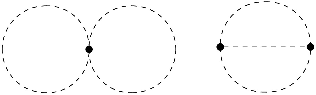
Figure A4. 2-loop vacuum diagrams.
$ \begin{split} V_\text{eff}^\text{2-loop} =& (3\lambda_1+3\lambda_2+\lambda_{12}){\cal{I}}_\text{bubble}^2(m_3)\\&-(3\kappa_1^2+3\kappa_2^2+\kappa_{12}^2){\cal{I}}_\text{sunset}(m_3)\,, \end{split} $

(D9) where [97]
$ \begin{split} &{\cal{I}}_\text{bubble}(m) = \frac{1}{(4\pi)^2}m^2\,, \\& {\cal{I}}_\text{sunset}(m) = \frac{1}{(4 \pi)^2} \left(\frac{1}{4 \epsilon} + \frac{1}{2} + \log{\frac{\mu}{3m}}\right)\,. \end{split} $

(D10) Altogether, and after removing
$ 1/\epsilon $ poles and constant terms, we obtain$ \begin{split} V_\text{eff}^\text{2-loop} =& \frac{1}{4\pi^2} \bigg\lbrace\left[\frac{9}{2}m_3^2c_{\varphi^6}-\left(1+2\log{\frac{\mu}{3m_3}}\right)\lambda_3^2\right]\varphi^\dagger\varphi\\&-9\left(1+2\log{\frac{\mu}{3m_3}}\right)c_{\varphi^6}\lambda_3(\varphi^\dagger\varphi)^2\bigg\rbrace\,. \end{split} $

(D11) -
The effective potential up to 2 loops within the 3D EFT can be expressed as follows:
$ \begin{split} V_\text{eff} &= m_3^2\varphi^\dagger\varphi+\lambda_3(\varphi^\dagger\varphi)^2+c_{\varphi^6}(\varphi^\dagger\varphi)^3+V_\text{eff}^\text{1-loop} + V_\text{eff}^\text{2-loop}\,, \end{split} $
(D1) where the 1-loop parts read
$ V_\text{eff}^\text{1-loop} = -\frac{1}{12 \pi} m_\text{eff}^3\,,\quad m^2_\text{eff} = 2\left[m_3^2+4\lambda_3 \varphi^\dagger\varphi+9c_{\varphi^6}(\varphi^\dagger\varphi)^2\right]\,, $
(D2) and we compute the 2-loop contribution following Jackiw's background-field method [96]. We limit the calculation to this loop order because it effectively eliminates nearly all renormalization scale dependence, while the finite contributions have a negligible impact on our numerical estimates.
To this aim, we write the Lagrangian in Eq. (2) in terms of the real components of
$ \varphi=(\varphi_1+i\varphi_2)/\sqrt{2} $ , and make the shift$ \varphi_1\to\varphi_1+\tilde{\varphi} $ . (This way, we avoid mass mixing, while the full dependence on φ can be later retrieved from$ O(2) $ invariance upon replacing$ \tilde{\varphi}\to\sqrt{2}\varphi $ .)Neglecting the dependence of the squared mass with
$ \tilde{\varphi} $ for simplicity, we obtain$ \begin{split} {\cal{L}}_{EFT} =& \frac{1}{2}m_3^2\varphi_1^2+\kappa_1\varphi_1^3+\lambda_1\varphi_1^4+\frac{1}{2}m_3^2\varphi_2^2+\lambda_2\varphi_2^4+\\&\kappa_{12}\varphi_1\varphi_2^2+\lambda_{12}\varphi_1^2\varphi_2^2+\cdots\,, \end{split} $
(D3) with
$ \kappa_1 =\lambda_3\tilde{\varphi}+\frac{5}{2}c_{\varphi^6}\tilde{\varphi}^3\,, $
(D4) $ \kappa_{12} = \lambda_3\tilde{\varphi}+\frac{3}{2}c_{\varphi^6}\tilde{\varphi}^3\,, $
(D5) $ \lambda_1 = \frac{1}{4}\lambda_3 + \frac{15}{8}c_{\varphi^6}\tilde{\varphi}^2\,, $
(D6) $ \lambda_2 = \frac{1}{4}\lambda_3 + \frac{3}{8}c_{\varphi^6}\tilde{\varphi}^2\,, $
(D7) $ \lambda_{12} = \frac{1}{2}\lambda_3 + \frac{9}{4}c_{\varphi^6}\tilde{\varphi}^2\,. $
(D8) Thus,
$ V_\text{eff}^\text{2-loop} $ is given by the sum of the 2-loop vacuum diagrams computed with these field-dependent couplings (see Fig. A4). We have
Figure A4. 2-loop vacuum diagrams.
$ \begin{split} V_\text{eff}^\text{2-loop} =& (3\lambda_1+3\lambda_2+\lambda_{12}){\cal{I}}_\text{bubble}^2(m_3)\\&-(3\kappa_1^2+3\kappa_2^2+\kappa_{12}^2){\cal{I}}_\text{sunset}(m_3)\,, \end{split} $
(D9) where [97]
$ \begin{split} &{\cal{I}}_\text{bubble}(m) = \frac{1}{(4\pi)^2}m^2\,, \\& {\cal{I}}_\text{sunset}(m) = \frac{1}{(4 \pi)^2} \left(\frac{1}{4 \epsilon} + \frac{1}{2} + \log{\frac{\mu}{3m}}\right)\,. \end{split} $
(D10) Altogether, and after removing
$ 1/\epsilon $ poles and constant terms, we obtain$ \begin{split} V_\text{eff}^\text{2-loop} =& \frac{1}{4\pi^2} \bigg\lbrace\left[\frac{9}{2}m_3^2c_{\varphi^6}-\left(1+2\log{\frac{\mu}{3m_3}}\right)\lambda_3^2\right]\varphi^\dagger\varphi\\&-9\left(1+2\log{\frac{\mu}{3m_3}}\right)c_{\varphi^6}\lambda_3(\varphi^\dagger\varphi)^2\bigg\rbrace\,. \end{split} $
(D11) -
We consider a second model consisting of a real scalar ϕ and a massless fermion ψ. The 4D Lagrangian in Minkowski space reads:
$ {\cal{L}}_\text{4} = \frac{1}{2}(\partial\phi)^2 - \frac{1}{2}m^2\phi^2 - \kappa\phi^3 - \lambda\phi^4 + \overline{\psi} i\not{\partial} \psi - y \phi\overline{\psi}\psi\,. $

(E1) As it was first studied in Ref. [46], this model allows for non-radiatively-induced PT owing to the presence of a non-
$ \mathbb{Z}_2 $ symmetric cubic term for the scalar which contributes at tree-level to the formation of a barrier within the 3D effective potential. In the aforementioned work, PT up to$ {\cal{O}}(y^5) $ were studied, following the power counting prescription$ \frac{m^2}{T^2} \sim \frac{|\mathbf{p}|^2}{T^2} \sim \lambda \sim \frac{\kappa}{T} \sim y^2 \,, $

(E2) where we have omitted numerical factors. This corresponds to 2-loop matching for the effective mass and 1-loop matching for the remaining Wilson coefficients in a 3D EFT that includes only renormalizable interactions. In Ref. [50], leading corrections in the form of 1-loop dimension-6 and dimension-8 operators in the 3D EFT were also considered.
Here, we take this computation, including only fermion loops, to
$ O(y^6) $ , except for the 3-loop contribution to the matching of the 3D effective mass. This limitation arises from the current lack of knowledge regarding the evaluation of 3-loop, mass dimension 2, fermionic, and mixed sum-integrals (see Appendix A for details). As a result, the mass term exhibits some renormalization-scale dependence.The scalar 3D EFT up to dimension-6 in Euclidean form reads [50]:
$ \begin{split} {\cal{L}}_\text{EFT} =& \frac{1}{2} K_3 (\partial\varphi)^2 + \frac{1}{2}m_3^2 \varphi^2 + \kappa_3 \varphi^3 + \lambda_3 \varphi^4\\& +c_{\varphi^6} \varphi^6 + r_{\partial^4 \varphi^2} \partial^2 \varphi \partial^2 \varphi + r_{\partial^2 \varphi^4} \varphi^3 \partial^2 \varphi\,. \end{split}$

(E3) First, the 3D scalar field φ is related to the zeroth Matsubara mode of ϕ through the following matching to the kinetic term
5 :$ \begin{split} K_3 &= 1 + \frac{1}{8 \pi^2} y^2 L_f \\ &\hphantom{= 1 } - \frac{1}{3072 \pi^4} y^4 \left( 36 L_f^2 + 60 L_f + 93 - 64 \log 2 + 70 \zeta(3) \right) \,. \end{split} $

(E4) We normalize canonically through
$ \varphi \to \varphi / \sqrt{K_3} $ . Again, we use the same notation for normalized and unnormalized WCs, and the normalized matching equations for the first read as follows:$ \begin{split} m_3^2 =& m^2 + y^2 \left( \frac{1}{6} T^2 - \frac{1}{8 \pi^2} m^2 L_f \right) \hphantom= + \frac{1}{768 \pi^2} y^2 \\ &\left\{ 8 T^2 \left( L_f - 8 \log 2 \right) + \frac{1}{4 \pi^2} m^2 \biggl[ 12 L_f^2 + 12 L_f \left( 1 + 48 \log 2 \right) \right.\end{split} $

$ \begin{split} & + 21 + 320 \log 2 + 70 \zeta(3) ] \} + \frac{1}{18432 \pi^4} y^6 \biggl[ 12 L_f^2 \\ & + 12 L_f \left( 5 + 16 \log 2 \right)+ 93 - 64 \log 2 + 70 \zeta(3) ] \,, \end{split} $

(E5) $ \begin{split} \kappa_3 &= \kappa \sqrt{T} - \frac{3}{16 \pi^2} \kappa y^2 \sqrt{T} L_f \\ &\hphantom= + \frac{1}{2048 \pi^4} \kappa y^4 \sqrt{T} \left( 96 L_f^2 + 60 L_f + 93 - 64 \log 2 + 70 \zeta(3) \right) \,, \end{split} $

(E6) $ \begin{split} \lambda_3 =& \lambda T + \frac{1}{16 \pi^2} y^4 T L_f - \frac{1}{4 \pi^2} \lambda y^2 T L_f \\&- \frac{1}{512 \pi^4} y^6 T \biggl[ 14 L_f^2 + 16 L_f + 24 + 7 \zeta(3) ] \\ & + \frac{1}{1536 \pi^4} \lambda y^4 T \biggl[ 108 L_f^2 + 60 L_f + 93 - 64 \log 2 + 70 \zeta(3) ] \,, \end{split} $

(E7) $ c_{\varphi^6} = - \frac{7 \zeta(3)}{192 \pi^4} y^6 \,,$

(E8) $ r_{\partial^4 \varphi^2} = - \frac{7 \zeta(3)}{384 \pi^4 T^2} y^2 \,,$

(E9) $ r_{\partial^2 \varphi^4} = \frac{35 \zeta(3)}{576 \pi^4 T} y^4 \,.$

(E10) The UV CT Lagrangian reads:
$ \begin{split} {\cal{L}}_{4, \rm ct} = &\frac{1}{2} \delta K_\phi (\partial\phi)^2 - \frac{1}{2} \delta m ^2\phi^2 - \delta\kappa \phi^3 - \delta\lambda \phi^4 \\&+ \delta K_\psi \overline{\psi} i\not{\partial} \psi - \delta y \phi\overline{\psi}\psi\,. \end{split}$

(E11) We compute the CTs up to
$ {\cal{O}}(y^6) $ , involving only fermion loops. To renormalize the matching equations, we need the following up to 2-loops:$ \delta K_\phi = - \frac{y^2}{8 \pi^2 \epsilon} + \frac{y^4}{512 \pi^4} \left( \frac{5}{\epsilon} - \frac{6}{\epsilon^2} \right) \,, $

(E12) $ \delta m^{2} = \frac{1}{128 \pi^4} y^4 m^2 \left( \frac{1}{\epsilon} - \frac{3}{\epsilon^2} \right) \,, $

(E13) $ \delta \lambda = -\frac{y^4}{16 \pi^2 \epsilon} + \frac{y^6}{256 \pi^4} \left( \frac{4}{\epsilon} - \frac{3}{\epsilon^2} \right) \,, $

(E14) while the rest are only needed up to 1-loop:
$ \delta \kappa = 0\,, \quad \delta K_\psi = -\frac{y^2}{32 \pi^2 \epsilon} \,, \quad \delta y = \frac{y^3}{16 \pi^2 \epsilon} \,. $

(E15) In contrast, in Euclidean space, the CT Lagrangian of the 3D Lagrangian reads:
$ \begin{split} {\cal{L}}_\text{EFT, ct} = & \frac{1}{2} \delta K_\varphi (\partial\varphi)^2 + \frac{1}{2} \delta m_3{}^2 \varphi^2 + \delta \kappa_3 \varphi^3 + \delta \lambda_3 \varphi^4 + \delta c_{\varphi^6} \varphi^6 \\ &+ \delta r_{\partial^4 \varphi^2} \partial^2 \varphi \partial^2 \varphi + \delta r_{\partial^2 \varphi^4} \varphi^3 \partial^2 \varphi\,, \end{split} $

(E16) and the only non-vanishing CT up to
$ {\cal{O}}(y^6) $ is:$ \delta m_3{}^{2} = \frac{3}{2 \pi^2 \epsilon} \lambda_3^2 \,.$

(E17) In the matching, we see that the UV CTs alone cancel all
$ \epsilon $ poles, and no temperature-dependent poles remain. Indeed, up to$ {\cal{O}}(y^6) $ , and without λ and κ insertions, this 3D CT does not contribute upon the substitution of the matching relations. This serves as a cross-check of our matching computation. -
We consider a second model consisting of a real scalar ϕ and a massless fermion ψ. The 4D Lagrangian in Minkowski space reads:
$ {\cal{L}}_\text{4} = \frac{1}{2}(\partial\phi)^2 - \frac{1}{2}m^2\phi^2 - \kappa\phi^3 - \lambda\phi^4 + \overline{\psi} i\not{\partial} \psi - y \phi\overline{\psi}\psi\,. $
(E1) As it was first studied in Ref. [46], this model allows for non-radiatively-induced PT owing to the presence of a non-
$ \mathbb{Z}_2 $ symmetric cubic term for the scalar which contributes at tree-level to the formation of a barrier within the 3D effective potential. In the aforementioned work, PT up to$ {\cal{O}}(y^5) $ were studied, following the power counting prescription$ \frac{m^2}{T^2} \sim \frac{|\mathbf{p}|^2}{T^2} \sim \lambda \sim \frac{\kappa}{T} \sim y^2 \,, $
(E2) where we have omitted numerical factors. This corresponds to 2-loop matching for the effective mass and 1-loop matching for the remaining Wilson coefficients in a 3D EFT that includes only renormalizable interactions. In Ref. [50], leading corrections in the form of 1-loop dimension-6 and dimension-8 operators in the 3D EFT were also considered.
Here, we take this computation, including only fermion loops, to
$ O(y^6) $ , except for the 3-loop contribution to the matching of the 3D effective mass. This limitation arises from the current lack of knowledge regarding the evaluation of 3-loop, mass dimension 2, fermionic, and mixed sum-integrals (see Appendix A for details). As a result, the mass term exhibits some renormalization-scale dependence.The scalar 3D EFT up to dimension-6 in Euclidean form reads [50]:
$ \begin{split} {\cal{L}}_\text{EFT} =& \frac{1}{2} K_3 (\partial\varphi)^2 + \frac{1}{2}m_3^2 \varphi^2 + \kappa_3 \varphi^3 + \lambda_3 \varphi^4\\& +c_{\varphi^6} \varphi^6 + r_{\partial^4 \varphi^2} \partial^2 \varphi \partial^2 \varphi + r_{\partial^2 \varphi^4} \varphi^3 \partial^2 \varphi\,. \end{split}$
(E3) First, the 3D scalar field φ is related to the zeroth Matsubara mode of ϕ through the following matching to the kinetic term
5 :$ \begin{split} K_3 &= 1 + \frac{1}{8 \pi^2} y^2 L_f \\ &\hphantom{= 1 } - \frac{1}{3072 \pi^4} y^4 \left( 36 L_f^2 + 60 L_f + 93 - 64 \log 2 + 70 \zeta(3) \right) \,. \end{split} $
(E4) We normalize canonically through
$ \varphi \to \varphi / \sqrt{K_3} $ . Again, we use the same notation for normalized and unnormalized WCs, and the normalized matching equations for the first read as follows:$ \begin{split} m_3^2 =& m^2 + y^2 \left( \frac{1}{6} T^2 - \frac{1}{8 \pi^2} m^2 L_f \right) \hphantom= + \frac{1}{768 \pi^2} y^2 \\ &\left\{ 8 T^2 \left( L_f - 8 \log 2 \right) + \frac{1}{4 \pi^2} m^2 \biggl[ 12 L_f^2 + 12 L_f \left( 1 + 48 \log 2 \right) \right.\end{split} $
$ \begin{split} & + 21 + 320 \log 2 + 70 \zeta(3) ] \} + \frac{1}{18432 \pi^4} y^6 \biggl[ 12 L_f^2 \\ & + 12 L_f \left( 5 + 16 \log 2 \right)+ 93 - 64 \log 2 + 70 \zeta(3) ] \,, \end{split} $
(E5) $ \begin{split} \kappa_3 &= \kappa \sqrt{T} - \frac{3}{16 \pi^2} \kappa y^2 \sqrt{T} L_f \\ &\hphantom= + \frac{1}{2048 \pi^4} \kappa y^4 \sqrt{T} \left( 96 L_f^2 + 60 L_f + 93 - 64 \log 2 + 70 \zeta(3) \right) \,, \end{split} $
(E6) $ \begin{split} \lambda_3 =& \lambda T + \frac{1}{16 \pi^2} y^4 T L_f - \frac{1}{4 \pi^2} \lambda y^2 T L_f \\&- \frac{1}{512 \pi^4} y^6 T \biggl[ 14 L_f^2 + 16 L_f + 24 + 7 \zeta(3) ] \\ & + \frac{1}{1536 \pi^4} \lambda y^4 T \biggl[ 108 L_f^2 + 60 L_f + 93 - 64 \log 2 + 70 \zeta(3) ] \,, \end{split} $
(E7) $ c_{\varphi^6} = - \frac{7 \zeta(3)}{192 \pi^4} y^6 \,,$
(E8) $ r_{\partial^4 \varphi^2} = - \frac{7 \zeta(3)}{384 \pi^4 T^2} y^2 \,,$
(E9) $ r_{\partial^2 \varphi^4} = \frac{35 \zeta(3)}{576 \pi^4 T} y^4 \,.$
(E10) The UV CT Lagrangian reads:
$ \begin{split} {\cal{L}}_{4, \rm ct} = &\frac{1}{2} \delta K_\phi (\partial\phi)^2 - \frac{1}{2} \delta m ^2\phi^2 - \delta\kappa \phi^3 - \delta\lambda \phi^4 \\&+ \delta K_\psi \overline{\psi} i\not{\partial} \psi - \delta y \phi\overline{\psi}\psi\,. \end{split}$
(E11) We compute the CTs up to
$ {\cal{O}}(y^6) $ , involving only fermion loops. To renormalize the matching equations, we need the following up to 2-loops:$ \delta K_\phi = - \frac{y^2}{8 \pi^2 \epsilon} + \frac{y^4}{512 \pi^4} \left( \frac{5}{\epsilon} - \frac{6}{\epsilon^2} \right) \,, $
(E12) $ \delta m^{2} = \frac{1}{128 \pi^4} y^4 m^2 \left( \frac{1}{\epsilon} - \frac{3}{\epsilon^2} \right) \,, $
(E13) $ \delta \lambda = -\frac{y^4}{16 \pi^2 \epsilon} + \frac{y^6}{256 \pi^4} \left( \frac{4}{\epsilon} - \frac{3}{\epsilon^2} \right) \,, $
(E14) while the rest are only needed up to 1-loop:
$ \delta \kappa = 0\,, \quad \delta K_\psi = -\frac{y^2}{32 \pi^2 \epsilon} \,, \quad \delta y = \frac{y^3}{16 \pi^2 \epsilon} \,. $
(E15) In contrast, in Euclidean space, the CT Lagrangian of the 3D Lagrangian reads:
$ \begin{split} {\cal{L}}_\text{EFT, ct} = & \frac{1}{2} \delta K_\varphi (\partial\varphi)^2 + \frac{1}{2} \delta m_3{}^2 \varphi^2 + \delta \kappa_3 \varphi^3 + \delta \lambda_3 \varphi^4 + \delta c_{\varphi^6} \varphi^6 \\ &+ \delta r_{\partial^4 \varphi^2} \partial^2 \varphi \partial^2 \varphi + \delta r_{\partial^2 \varphi^4} \varphi^3 \partial^2 \varphi\,, \end{split} $
(E16) and the only non-vanishing CT up to
$ {\cal{O}}(y^6) $ is:$ \delta m_3{}^{2} = \frac{3}{2 \pi^2 \epsilon} \lambda_3^2 \,.$
(E17) In the matching, we see that the UV CTs alone cancel all
$ \epsilon $ poles, and no temperature-dependent poles remain. Indeed, up to$ {\cal{O}}(y^6) $ , and without λ and κ insertions, this 3D CT does not contribute upon the substitution of the matching relations. This serves as a cross-check of our matching computation.
Phase transitions in dimensional reduction up to three loops
- Received Date: 2025-06-17
- Available Online: 2025-12-15
Abstract: We perform the first computation of phase-transition parameters to cubic order in


 DownLoad: