


 Abstract
 HTML
HTML Reference
 Related
 PDF
PDF


-
The Hawking radiation of a black hole actually traverses the gravitational field surrounding the black hole, modifying the spectrum of the radiation and rendering it distinct from the ideal black-body radiation [1−3]. The grey-body factor accounts for the discrepancy between the actual spectrum of black hole radiation and ideal case of perfect black-body radiation, and it modifies the purely theoretical prediction of the Hawking radiation spectrum. This factor is a frequency-dependent function that characterizes the probability that radiation at a given frequency can traverse the potential barrier surrounding the black hole and escape to infinity. Due to the strong gravitational field of a black hole, part of the radiation is reflected back into the black hole or absorbed by it, which results in a weaker observed radiation intensity. Therefore, the grey-body factor is pivotal in refining the description of Hawking radiation, which brings the theoretical calculations closer to the actual physical conditions [2−12].
The QNMs as a response of a black hole under perturbations can be used to reveal the intrinsic characteristics of black holes and compact stars such as the mass and spin [13−18]. Meanwhile, it is an important tool to analyze gravitational waves during the ringdown process [15, 19−29]. Recently, QNMs have been widely studied as an effective means of probing the internal structure and quantum effects of regular black holes [10, 30−43]. Regular black holes represent a special class of black hole models characterized by the absence of a singularity at their center [44−47]. Unlike standard black holes in general relativity, regular black holes circumvent the singularity problem, thereby avoiding the physical conundrum of infinite density and curvature at the core of traditional black holes [48, 49]. The concept of regular black holes was initially proposed based on phenomenological considerations, which suggests that quantum gravitational effects can eliminate the singularity under extreme conditions, thereby resulting in a more "regular" internal structure of the black hole [50−53]. Subsequently, it is shown that regular black holes can be constructed in various ways. One approach involves solving Einstein field equations with exotic matter that violates classical energy conditions, thereby obtaining black hole solutions without singularities [54−58]. Another approach is constructing regular black hole solutions by considering modified Einstein equations that incorporate quantum gravitational corrections, which typically arise from quantum gravity theories or semi-classical gravitational theories [59−62]. The study of regular black holes not only provides new insights into resolving the singularity problem of traditional black holes but also offers a significant theoretical framework for exploring the manifestations of quantum gravitational effects in strong gravitational fields.
In fact, both the QNMs and grey-body factors are two important quantities that describe the properties of black holes with different boundary conditions. Interestingly, in [63], the correspondence between the QNMs and grey-body factor is established with the help of WKB expansion. A formula is derived that allows one to compute the grey-body factor from the fundamental mode and the first overtone of the QNMs for large values of the angular number l. In the eikonal limit, the grey-body factor is solely determined by the fundamental mode. Currently, this correspondence in the high-frequency regime has been extended to spherically symmetric black holes [63], axisymmetric black holes [64], quantum-corrected black holes [65], and other types of black holes [66−69]. In this study, we intend to construct this correspondence for a sort of regular black hole proposed in [70]. These regular black holes are characterized by sub-Planckian curvature and a Minkowski core, unlike the ordinary Bardeen and Hayward black holes that possess a de-Sitter core.
Our paper is organized as follows: In Section II, we briefly introduce regular black holes with sub-Planckian curvature and a Minkowskian core. In Section III, we compute the QNMs of regular black holes under gravitational perturbations. In Section IV, we focus on the grey-body factors and numerically check the correspondence between the QNMs and grey-body factors. In Section V, we present the summary and conclusions.
-
The Hawking radiation of a black hole actually traverses the gravitational field surrounding the black hole, which modifies the spectrum of the radiation and renders it distinct from the ideal black-body radiation [2−4]. The grey-body factor accounts for the discrepancy between the actual spectrum of black hole radiation and the ideal case of perfect black-body radiation, and it modifies the purely theoretical prediction of the Hawking radiation spectrum. It is a frequency-dependent function that characterizes the probability that radiation at a given frequency can traverse the potential barrier surrounding the black hole and escape to infinity. Due to the strong gravitational field of a black hole, part of the radiation is reflected back into the black hole or absorbed by it, resulting in a weaker observed radiation intensity. Therefore, the grey-body factor is pivotal in refining the description of Hawking radiation, bringing theoretical calculations closer to the actual physical conditions [3−13].
On the other hand, the QNMs as the response of a black hole under the perturbations can be used to reveal the intrinsic characteristics of black holes and compact stars, such as the mass and spin [14−19]. At the same time, it is an important tool for analyzing gravitational waves during the ringdown process [16, 20−30]. Recently, the QNMs have also been widely studied as an effective means of probing the internal structure and quantum effects of regular black holes [11, 31−44]. Regular black holes represent a special class of black hole models characterized by the absence of a singularity at their center [45−48]. Unlike standard black holes in general relativity, regular black holes circumvent the singularity problem, thereby avoiding the physical conundrum of infinite density and curvature at the core of traditional black holes [49, 50]. The concept of regular black holes was initially proposed based on phenomenological considerations, suggesting that quantum gravitational effects would eliminate the singularity under extreme conditions, resulting in a more “regular” internal structure of the black hole [51−54]. Subsequently, it is shown that regular black holes can be constructed in various ways. One approach involves solving the Einstein field equations with exotic matter that violates classical energy conditions, thereby obtaining black hole solutions without singularities [55−59]. Another approach is to construct regular black hole solutions by considering modified Einstein equations that incorporate quantum gravitational corrections, which typically arise from quantum gravity theories or semi-classical gravitational theories [60−63]. The study of regular black holes not only provides new insights into resolving the singularity problem of traditional black holes but also offers a significant theoretical framework for exploring the manifestations of quantum gravitational effects in strong gravitational fields.
As a matter of fact, both the QNMs and the grey-body factors are two important quantities that describe the properties of black holes with different boundary conditions. Interestingly, in [1], the correspondence between the QNMs and the grey-body factor is established with the help of WKB expansion. Specifically, a formula is derived that allows one to compute the grey-body factor from the fundamental mode and the first overtone of the QNMs for large values of the angular number l. In particular, in the eikonal limit the grey-body factor is solely determined by the fundamental mode. Currently, this correspondence in the high-frequency regime has been extended to spherically symmetric black holes [1], axisymmetric black holes [64], quantum-corrected black holes [65], and other types of black holes [66−69]. In this paper we intend to construct this correspondence for a sort of regular black hole proposed in [70]. These regular black holes are characterized by sub-Planckian curvature and a Minkowski core, unlike the ordinary Bardeen and Hayward black holes that possess a de-Sitter core.
Our work is organized as follows. In Section II, we briefly introduce regular black holes with sub-Planckian curvature and a Minkowskian core. In Section III, we compute the QNMs of regular black holes under gravitational perturbations. In Section IV, we focus on the grey-body factors and numerically check the correspondence between the QNMs and grey-body factors. Section V is the summary and conclusions.
-
In this section, we briefly introduce the regular black hole which was originally proposed in [70]. This kind of regular black hole is characterized by the sub-Planckian curvature as well as an asymptotically Minkowski core, which is realized by introducing an exponentially suppressing gravity potential [51]. Specifically, the spherically symmetric metric of this sort of regular black holes takes the form as follows
$ \begin{split} d s^{2}=-f(r) d t^{2}+\frac{1}{f(r)}d r^{2}+r^{2}\left(d \theta^{2}+\sin ^{2} \theta d \phi^{2}\right), \end{split} $

(1) where the function
$ f(r) $ is given by$ \begin{split} f(r)=1+2\psi(r)=1-\frac{2M}re^{\frac{-\alpha_0M^x}{r^c}}, \end{split} $

(2) where M is understood as the mass of black hole and the parameters x, c,
$ \alpha_0 $ are all the dimensionless parameters1 . Here the value of$ \alpha_0 $ reflects the degree of deviation from the Newtonian potential and characterizes the corrections due to the effects of quantum gravity [51, 52, 70]. A class of regular black holes with sub-Planckian Kretschmann curvature can be constructed by varying the parameters x and c, subject to the conditions$ c \geqslant x \geqslant c/3 $ and$ c\geqslant 2 $ . In particular, the cases ($ x=2/3 $ ,$ c=2 $ ) and ($ x=1 $ ,$ c=3 $ ) represent two typical examples of such regular black holes, whose asymptotic behavior at spatial infinity coincides with that of the well-known Bardeen and Hayward black holes, respectively. The theoretical properties and the observation signature of this sort of regular black holes have been recently investigated in [42, 44, 71−74]. Without loss of generality, in this paper we will firstly focus on the case of$ x=2/3 $ and$ c=2 $ , which exhibits the same asymptotic behavior as Bardeen black hole at infinity, and then present a discussion on other cases with different values of x and c. At large scales where$ r\gg\sqrt{\alpha_{0}}M^{1/3} $ , the function$ f(r) $ of regular black holes can be expanded as the following form$ \begin{split} f(r)=\;&1+2\psi(r)=1-\frac{2M}{r}e^{-\alpha_0M^{2/3}/r^2}\cong1\\ &-\frac{2M}{r}\left(1-\frac{\alpha_0M^{2/3}}{r^2}+\cdots\right). \end{split} $

(3) On the other hand, the function ψ of the Bardeen black hole has the form
$ \begin{split} \psi(r)=-\dfrac{Mr^2}{\left(\dfrac{2}{3}\alpha_0M^{2/3}+r^2\right)^{3/2}}. \end{split} $

(4) So, at large scales the function
$ f(r) $ asymptotically behaves as$ \begin{split} f(r)=\;&1+2\psi(r)=1-\dfrac{2Mr^2}{\left(\dfrac{2}{3}\alpha_0M^{2/3}+r^2\right)^{3/2}}\cong1\\ &-\dfrac{2M}{r}\left(1-\dfrac{\alpha_0M^{2/3}}{r^2}+\cdots\right), \end{split} $

(5) which is the same as the regular black hole with
$ x=2/3 $ and$ c=2 $ . The case with$ x=1 $ and$ c=3 $ has been discussed in detail in [70]. In this case, the Hawking temperature is given by$ f'(r_h)/(4\pi) $ , and to keep its positivity one finds that the value of$ \alpha_0 $ should satisfy$ \begin{split} \alpha_0\leqslant\frac{2M^\frac{4}{3}}{e}. \end{split} $

(6) Next we consider the QNMs of the gravitational field perturbations over this regular black hole. Previously, the perturbations of the scalar field with spin zero as well as the electromagnetic field with spin one have been investigated in detail in [44]. By means of the separation of variables, the axial perturbation equation can be simplified to a Schrödinger-like equation :
$ \begin{split} \frac{\partial^2\Psi}{\partial r_*^2}+(\omega^2-V_{eff})\Psi=0\:, \end{split} $

(7) where the tortoise coordinate
$ r_* $ is defined in relation to the radial coordinate r by the equation:$ \begin{split} \frac{dr_*}{dr} = \frac{1}{f(r)}. \end{split} $

(8) The effective potential under gravitational perturbations has the form
$ \begin{split} V_{eff}(r) = f(r) \left( \frac{l(l + 1)}{r^2} - \frac{3 f'(r)}{r} \right), \end{split} $

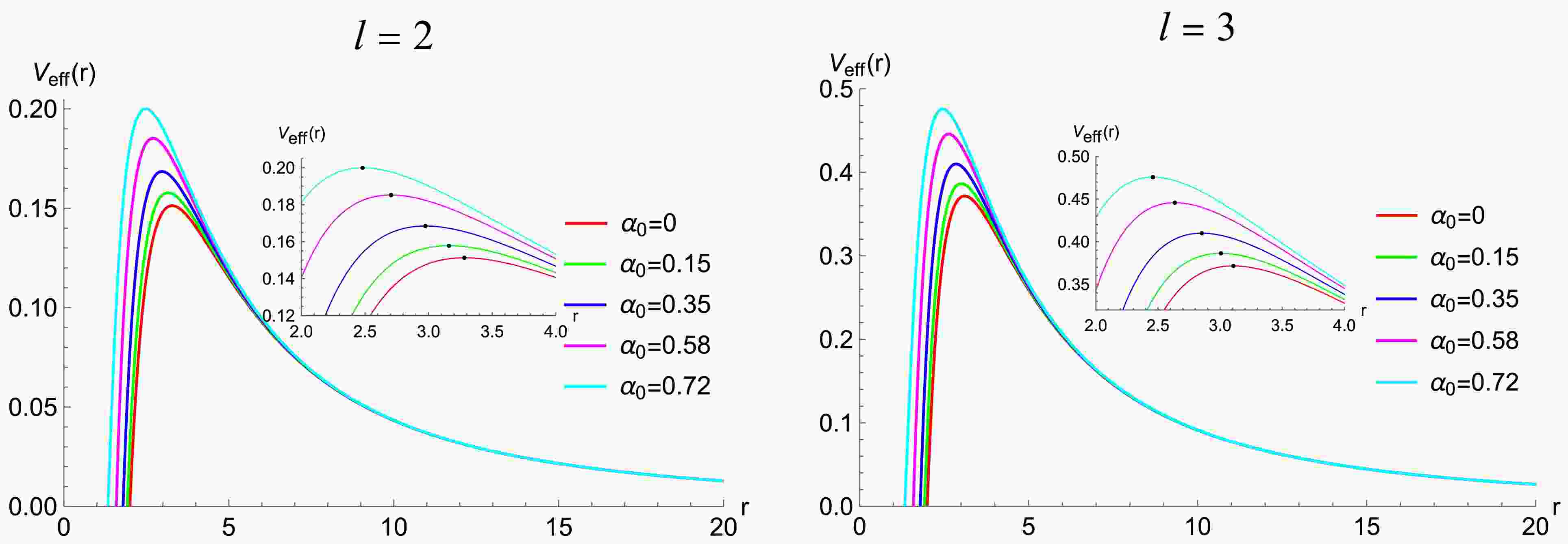
(9) where l is the angular number. In Fig. 1, we plot the effective potential
$ V_{eff}(r) $ of the gravitational field with different deviation parameters$ \alpha_0 $ . It shows that the effective potential is always positive, indicating that the spacetime of this regular BH is stable under the gravitational perturbation. From Fig. 1, we note two characteristics of the effective potential. First, when l is fixed, the peak of the effective potential increases as the deviation parameter$ \alpha_0 $ increases. Second, when$ \alpha_0 $ is fixed, the maximum of the effective potential increases as l increases.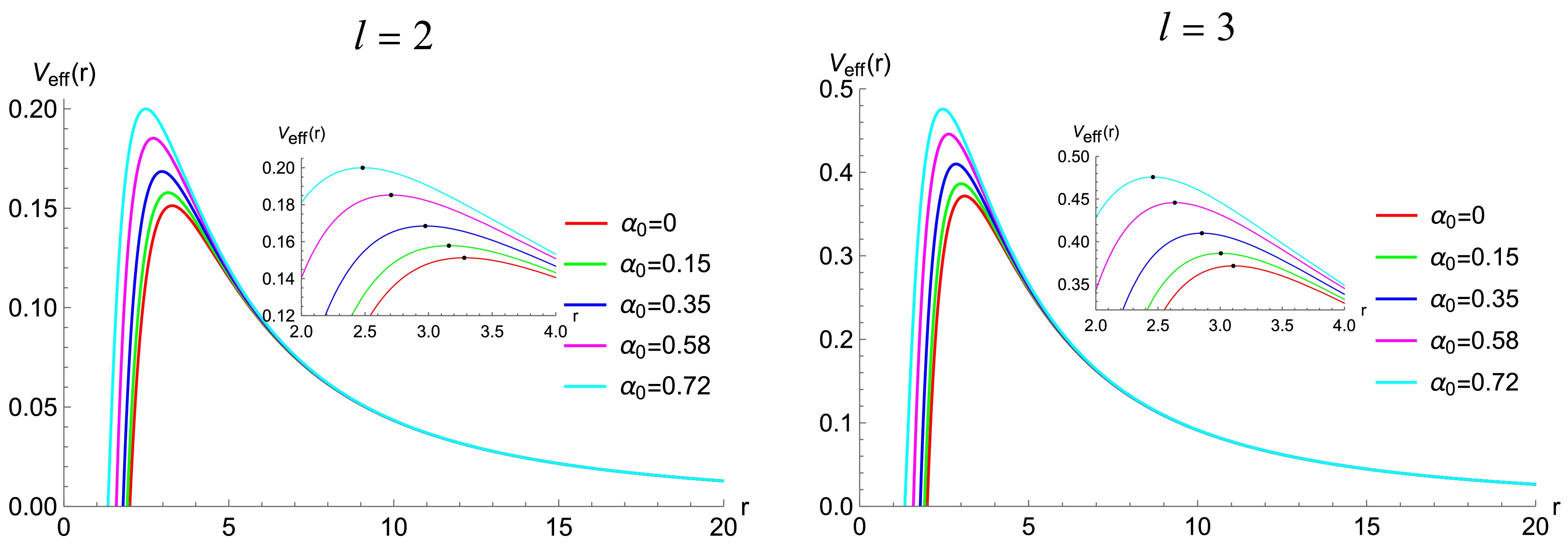
Figure 1. The effective potential
$ V_{eff}(r) $ of the gravitational field with different deviation parameters$ \alpha_0 $ . The black dot represents the maximum value of the$ V_{{eff}}(r) $ . -
In this section, we briefly introduce the regular black hole which was originally proposed in [70]. This type of regular black hole is characterized by the sub-Planckian curvature as well as an asymptotically Minkowski core, which is realized by introducing an exponentially suppressing gravity potential [50]. Specifically, the spherically symmetric metric of this sort of regular black holes takes the form
$ \begin{split} {\rm d} s^{2}=-f(r) {\rm d} t^{2}+\frac{1}{f(r)}{\rm d} r^{2}+r^{2}\left({\rm d} \theta^{2}+\sin ^{2} \theta {\rm d} \phi^{2}\right), \end{split} $
(1) where the function
$ f(r) $ is given by$ \begin{split} f(r)=1+2\psi(r)=1-\frac{2M}r {\rm e}^{\frac{-\alpha_0M^x}{r^c}}, \end{split} $
(2) where M is the mass of the black hole and parameters x, c, and
$ \alpha_0 $ represent all dimensionless parameters1 . Here, the value of$ \alpha_0 $ reflects the degree of deviation from the Newtonian potential and characterizes the corrections caused by the effects of quantum gravity [50, 51, 70]. A class of regular black holes with sub-Planckian Kretschmann curvature can be constructed by varying the parameters x and c, subject to conditions$ c \geqslant x \geqslant c/3 $ and$ c\geqslant 2 $ . Cases ($ x=2/3 $ ,$ c=2 $ ) and ($ x=1 $ ,$ c=3 $ ) represent two typical examples of such regular black holes, whose asymptotic behavior at spatial infinity coincides with that of the well-known Bardeen and Hayward black holes, respectively. The theoretical properties and observation signature of this sort of regular black holes have been recently investigated in [41, 43, 71−74]. Without loss of generality, we first focus on the case of$ x=2/3 $ and$ c=2 $ , which exhibits the same asymptotic behavior as the Bardeen black hole at infinity, and then, we present a discussion on other cases with different values of x and c. At large scales where$ r\gg\sqrt{\alpha_{0}}M^{1/3} $ , the function$ f(r) $ of regular black holes can be expanded as$ \begin{split} f(r)=\;&1+2\psi(r)=1-\frac{2M}{r}{\rm e}^{-\alpha_0M^{2/3}/r^2}\\ \cong\; & 1 - \frac{2M}{r}\left(1-\frac{\alpha_0M^{2/3}}{r^2}+\cdots\right). \end{split} $
(3) The function ψ of the Bardeen black hole has the form
$ \begin{split} \psi(r)=-\dfrac{Mr^2}{\left(\dfrac{2}{3}\alpha_0M^{2/3}+r^2\right)^{3/2}}. \end{split} $
(4) Therefore, at large scales, the function
$ f(r) $ asymptotically behaves as$ \begin{split} f(r)=\;&1+2\psi(r)=1-\dfrac{2Mr^2}{\left(\dfrac{2}{3}\alpha_0M^{2/3}+r^2\right)^{3/2}}\cong1\\ &-\dfrac{2M}{r}\left(1-\dfrac{\alpha_0M^{2/3}}{r^2}+\cdots\right), \end{split} $
(5) which is the same as the regular black hole with
$ x=2/3 $ and$ c=2 $ . The case with$ x=1 $ and$ c=3 $ has been discussed in detail in [70]. In this case, the Hawking temperature is given by$ f'(r_h)/(4\pi) $ , and to keep its positivity, the value of$ \alpha_0 $ should satisfy$ \begin{split} \alpha_0\leqslant\frac{2M^\frac{4}{3}}{e}. \end{split} $
(6) Next, we consider the QNMs of the gravitational field perturbations over this regular black hole. Previously, the perturbations of the scalar field with spin zero as well as the electromagnetic field with spin one have been investigated in detail in [43]. By separating the variables, the axial perturbation equation can be simplified to a Schrödinger-like equation given as
$ \begin{split} \frac{\partial^2\Psi}{\partial r_*^2}+(\omega^2-V_{eff})\Psi=0\:, \end{split} $
(7) where the tortoise coordinate
$ r_* $ is defined in relation to the radial coordinate r by the equation$ \begin{split} \frac{{\rm d}r_*}{{\rm d}r} = \frac{1}{f(r)}. \end{split} $
(8) The effective potential under gravitational perturbations has the form
$ \begin{split} V_{\rm eff}(r) = f(r) \left( \frac{l(l + 1)}{r^2} - \frac{3 f'(r)}{r} \right), \end{split} $
(9) where l represents the angular number. In Fig. 1, we plot the effective potential
$ V_{\rm eff}(r) $ of the gravitational field with different deviation parameters$ \alpha_0 $ . The effective potential is always positive, indicating that the spacetime of this regular BH is stable under the gravitational perturbation. From Fig. 1, we note two characteristics of the effective potential. First, when l is fixed, the peak of the effective potential increases with an increase in the deviation parameter$ \alpha_0 $ . Second, when$ \alpha_0 $ is fixed, the maximum of the effective potential increases with an increase in l.
Figure 1. (color online) Effective potential
$ V_{\rm eff}(r) $ of the gravitational field with different deviation parameters$ \alpha_0 $ . The black dot represents the maximum value of$ V_{{\rm eff}}(r) $ . -
In this section, we investigate the QNMs of regular black holes with
$ x=2/3 $ and$ c=2 $ under gravitational perturbations. It is well known that the boundary conditions for QNMs are defined as follows:$ \Psi \sim e^{i\omega r_*} \quad r_* \to +\infty, $

(10a) $ \Psi \sim e^{-i\omega r_*} \quad r_* \to -\infty. $

(10b) The frequencies of QNMs can be determined by solving the wave equation in conjunction with the boundary conditions. In this section, we employ the WKB method and the pseudospectral method to compute the QNMs of the regular black hole under gravitational perturbations. The details of the pseudospectral method can be found in the appendix of [44]. Here we present the numerical results as below.
Tables 1 and 2 list the QNMs of
$ n=0 $ and$ n=1 $ for different values of the deviation parameter with using the WKB method and the pseudospectral method, respectively. The discrepancy between these two methods is minimal, which validates the accuracy of both approaches. For$ n=0 $ and$ n=1 $ , the QNMs exhibit a larger real part and a smaller imaginary part, indicating stronger oscillations and weaker damping in both cases. For different values of$ \alpha_0 $ , with the same overtone number n and angular number l, the QNMs frequency changes in a monotonic manner as$ \alpha_0 $ increases. Specifically, the real part of the QNMs frequency increases, while the absolute value of the imaginary part decreases.$ n=0 $ 

$ n=1 $ 

$ \alpha_0 $ 

WKB PS WKB PS 0 0.373619-0.088891I 0.373672-0.088962I 0.346297-0.27348I 0.346711-0.273915I 0.15 0.381319-0.085311I 0.382617-0.08763I 0.352538-0.264144I 0.3586-0.269413I 0.3 0.39348-0.085922I 0.393707-0.085653I 0.3724-0.264948I 0.37302-0.262788I 0.5 0.410334-0.08219I 0.411063-0.08163I 0.390747-0.254688I 0.394524-0.249416I 2/e 0.441664-0.069059I 0.437952-0.071494I 0.437082-0.196175I 0.420167-0.217681I Table 1. The fundamental mode and the first overtone mode under gravitational perturbations for different values of
$ \alpha_0 $ , where$ l=2 $ .$ n=0 $ 

$ n=1 $ 

$ \alpha_0 $ 

WKB PS WKB PS 0 0.599443-0.092703I 0.599443-0.092703I 0.582642-0.28129I 0.582644-0.281298I 0.15 0.611912-0.091489I 0.611485-0.091532I 0.596558-0.277408I 0.596085-0.277538I 0.3 0.62612-0.089774I 0.62623-0.089753I 0.612282-0.27194 I 0.612408-0.27186I 0.5 0.648871-0.086103I 0.648869-0.086098I 0.636886-0.260279I 0.636885-0.260262I 2/e 0.684759-0.076612I 0.683071-0.077217I 0.670626-0.231287I 0.669319-0.233063I Table 2. The fundamental mode and the first overtone mode under gravitational perturbations for different values of
$ \alpha_0 $ , where$ l=3 $ .Next we turn to the higher overtone modes. It is important to emphasize that the WKB method exhibits high precision only when the overtone number n is relatively small. Therefore, for data where
$ n \geqslant 2 $ , we employ the pseudospectral method for the calculations. From Tables 3 and 4, it can be seen that higher overtone QNMs have smaller real parts and larger imaginary parts which is in contrast to the case of$ n=0 $ and$ n=1 $ , implying that these overtone modes are damping rapidly. Furthermore, for a given l and$ \alpha_0 $ , the real part of the frequency becomes smaller as the overtone number n increases, while the imaginary part becomes larger. On the other hand, if we fix$ \alpha_0 $ and n, but increase l, then from Tables 3 ($ l=2 $ ) and 4 ($ l=3 $ ), we find that the real part of the QNMs increases as well. This is understandable because as l increases, the effective potential increases as well (refer to Fig. 1), implying that a larger frequency is required to overcome the potential barrier. Finally, when we examine the effects of the variation of$ \alpha_0 $ , we find for low overtone numbers, the real and imaginary part of the QNMs change monotonically with increasing$ \alpha_0 $ ; however, for high overtone numbers, this monotonic behavior disappears. To gain an intuitive picture for the influence of$ \alpha_0 $ on QNMs, we demonstrate the change of the QNMs frequency with the deviation parameter$ \alpha_0 $ in Fig. 2 for$ l=2 $ and Fig. 3 for$ l=3 $ , respectively. In each plot with a fixed n and l, the variation of the frequency with$ \alpha_0 $ forms a trajectory on the frequency plane as$ \alpha_0 $ runs from$ 0 $ to$ 2/e $ , where the left ending point corresponds to$ \alpha_0=0 $ (representing the Schwarzschild black hole), while the right ending point represents$ \alpha_0=2/e $ .$ \alpha_0 $ 

$ n=2 $ 

$ n=3 $ 

$ n=4 $ 

$ n=5 $ 

0 0.301053-0.478277I 0.251505-0.705148I 0.207515-0.946845I 0.169303-1.19561I 0.15 0.318382-0.468975I 0.275574-0.689117I 0.239356-0.923063I 0.211068-1.163552I 0.3 0.338577-0.455611I 0.302014-0.666708I 0.271387-0.890632I 0.248115-1.121092I 0.5 0.366331-0.429253I 0.334302-0.623543I 0.303987-0.829115I 0.276284-1.041561I 2/e 0.384833-0.374182I 0.334921-0.549445I 0.279652-0.749675I 0.23127-0.972254I Table 3. higher overtone modes under gravitational perturbations for different values of
$ \alpha_0 $ , where$ l=2 $ .$ \alpha_0 $ 

$ n=2 $ 

$ n=3 $ 

$ n=4 $ 

$ n=5 $ 

0 0.551685-0.479093I 0.511962-0.690337I 0.470174-0.915649I 0.431386-1.15215I 0.15 0.567742-0.471985I 0.531359-0.678713I 0.492955-0.898341I 0.457169-1.128414I 0.3 0.586941-0.461381I 0.554056-0.661643I 0.518891-0.873288I 0.485507-1.094386I 0.5 0.614486-0.440002I 0.584606-0.627843I 0.550755-0.824515I 0.515777-1.02902I 2/e 0.642013-0.393333I 0.601909-0.561527I 0.551089-0.741569I 0.493761-0.936819I Table 4. higher overtone modes under gravitational perturbations for different values of
$ \alpha_0 $ , where$ l=3 $ 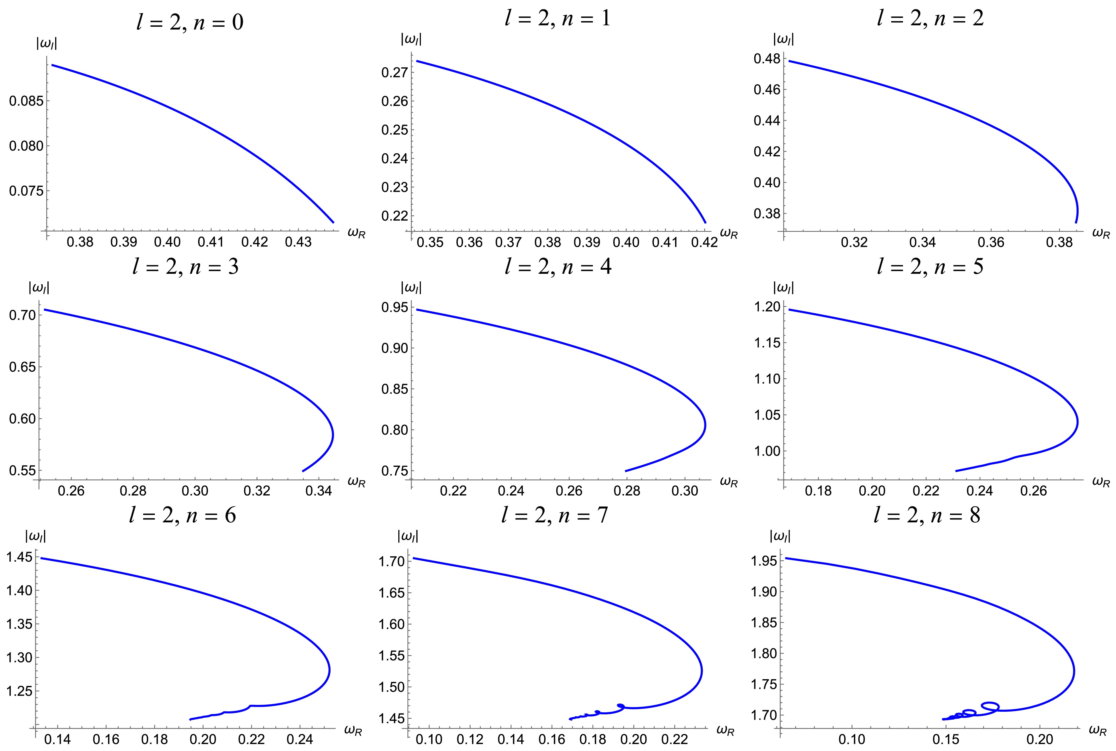
Figure 2. The trajectory of the QNMs with the variation of
$ \alpha_0 $ on the frequency plane with$ l=2 $ under gravitational field perturbations.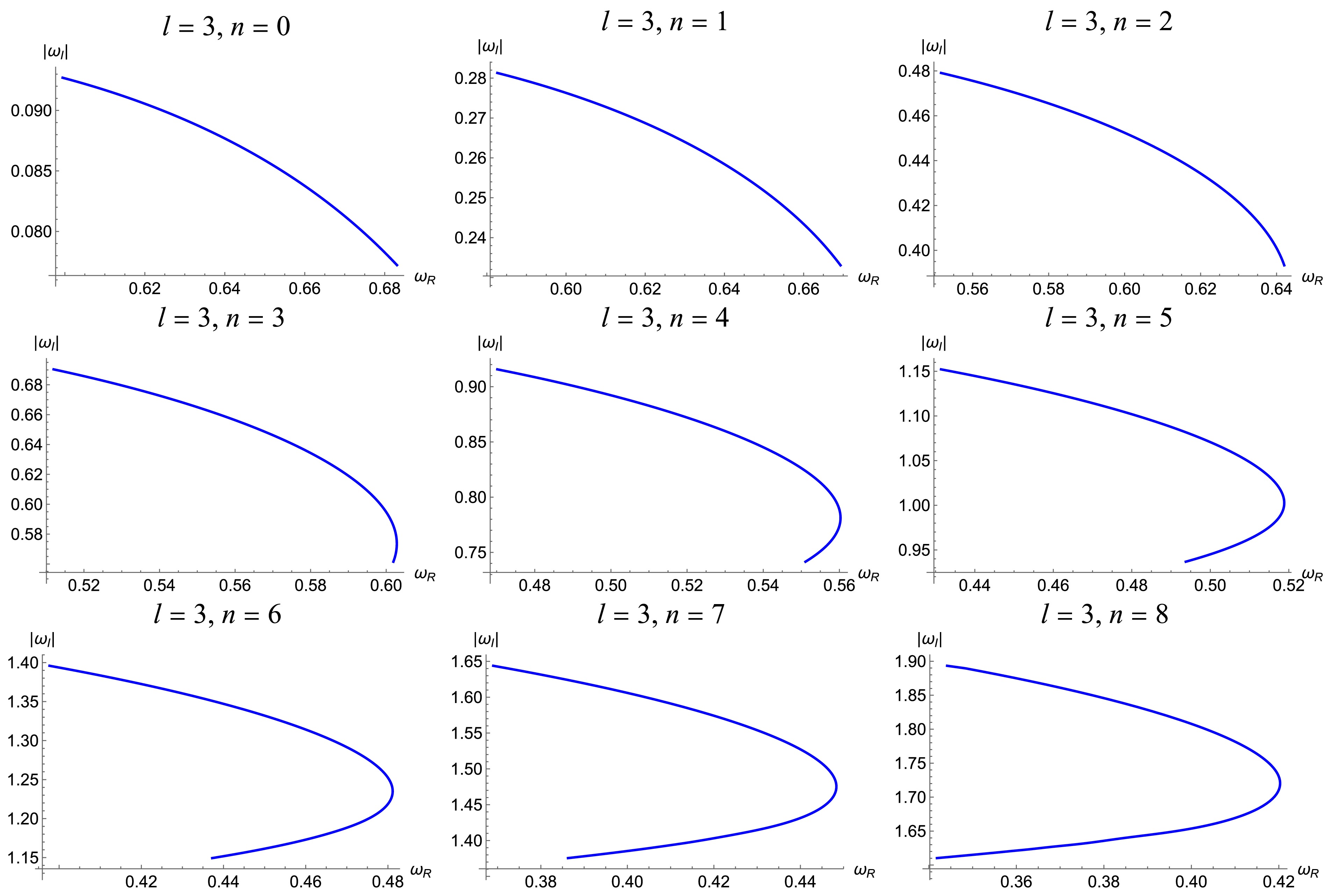
Figure 3. The trajectory of the QNMs with the variation of
$ \alpha_0 $ on the frequency plane with$ l=3 $ under gravitational field perturbation.From Figs. 2 and 3, it is observed that, overall, as the deviation parameter
$ \alpha_0 $ increases, the real part of the QNMs increases while the absolute value of the imaginary part decreases for lower overtone numbers. This monotonic behavior persists for cases such as$ l = 2 $ ,$ n = 0, 1 $ and$ l = 3 $ ,$ n = 0, 1, 2 $ . However, for higher overtone numbers, the QNMs trajectories begin to exhibit non-monotonic behavior. More importantly, in the cases of$ l = 2 $ and$ n = 6, 7, 8 $ , we clearly observe the emergence of spiral structures on the complex frequency plane. This phenomenon is similar to the results reported in Refs. [42, 44], where spiral trajectories were found for scalar and electromagnetic perturbations with$ l = 0 $ and$ l = 1 $ . In contrast, our results demonstrate that such spiral structures can also arise under gravitational perturbations when the overtone number n is sufficiently large, even with$ l \geq 2 $ .Figs. 4 and 5 display the real and imaginary parts of the QNMs as functions of the deviation parameter
$ \alpha_0 $ respectively, offering a complementary perspective to the full QNMs trajectories shown in the complex frequency plane in Figs. 2 and 3. For$ l = 2 $ and$ n = 6, 7, 8 $ , the real part exhibits pronounced oscillatory behavior, while the imaginary part shows milder fluctuations. These oscillations reflect the same underlying dynamics responsible for the spiral structures observed in Fig. 2. For$ l = 3 $ , no such oscillatory behavior is observed in either component up to$ n = 8 $ , but based on the trend at$ l = 2 $ , it is expected that oscillations—and spiral structures in the complex frequency plane—may emerge at larger overtone numbers. These observations reinforce the connection between high overtone numbers and the development of non-monotonic or spiral features in the QNMs spectrum.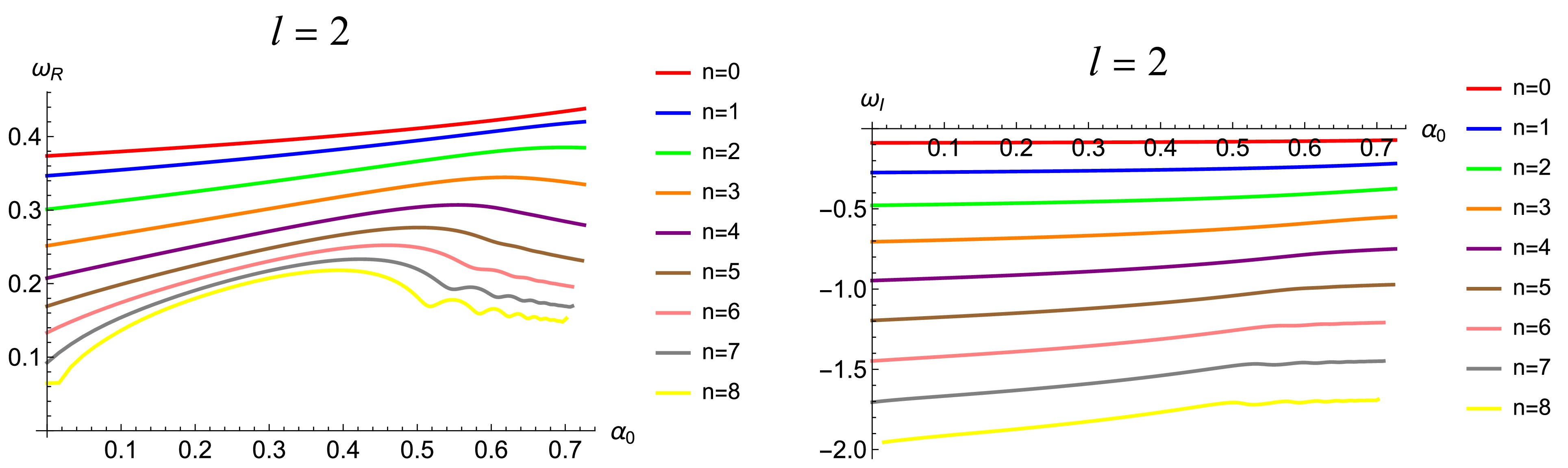
Figure 4. The real and imaginary parts of QNMs as the function of
$ \alpha_0 $ with$ l=2 $ under gravitational field perturbation.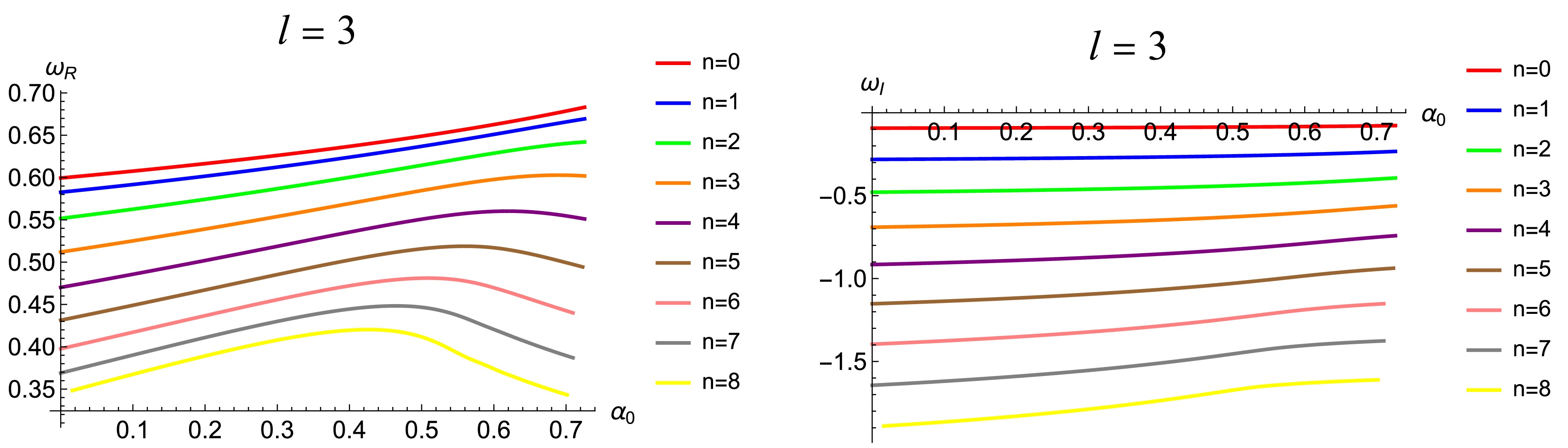
Figure 5. The real and imaginary parts of QNMs as the function of
$ \alpha_0 $ with$ l=3 $ gravitational field perturbation. -
In this section, we investigate the QNMs of regular black holes with
$ x=2/3 $ and$ c=2 $ under gravitational perturbations. It is well known that the boundary conditions for QNMs are defined as$ \Psi \sim {\rm e}^{{\rm i}\omega r_*} \quad r_* \to +\infty, $
(10a) $ \Psi \sim {\rm e}^{-{\rm i}\omega r_*} \quad r_* \to -\infty. $
(10b) The frequencies of QNMs can be determined by solving the wave equation in conjunction with the boundary conditions. We employ the WKB and pseudospectral methods to compute the QNMs of the regular black hole under gravitational perturbations. The details of the pseudospectral method can be found in the appendix of [43]. Here, we present the numerical results as below.
Tables 1 and 2 list the QNMs of
$ n=0 $ and$ n=1 $ for different values of the deviation parameter using the WKB and pseudospectral methods, respectively. The discrepancy between these two methods is minimal, which validates the accuracy of both approaches. For$ n=0 $ and$ n=1 $ , the QNMs exhibit a larger real part and a smaller imaginary part, indicating stronger oscillations and weaker damping in both cases. For different values of$ \alpha_0 $ with the same overtone number n and angular number l, the QNMs frequency changes in a monotonic manner with an increase in$ \alpha_0 $ . The real part of the QNMs frequency increases, whereas the absolute value of the imaginary part decreases.$ \alpha_0 $ $ n=0 $ $ n=1 $ WKB PS WKB PS 0 0.373619-0.088891I 0.373672-0.088962I 0.346297-0.27348I 0.346711-0.273915I 0.15 0.381319-0.085311I 0.382617-0.08763I 0.352538-0.264144I 0.3586-0.269413I 0.3 0.39348-0.085922I 0.393707-0.085653I 0.3724-0.264948I 0.37302-0.262788I 0.5 0.410334-0.08219I 0.411063-0.08163I 0.390747-0.254688I 0.394524-0.249416I 2/e 0.441664-0.069059I 0.437952-0.071494I 0.437082-0.196175I 0.420167-0.217681I Table 1. Fundamental mode and first overtone mode under gravitational perturbations for different values of
$ \alpha_0 $ , where$ l=2 $ .$ \alpha_0 $ $ n=0 $ $ n=1 $ WKB PS WKB PS 0 0.599443-0.092703I 0.599443-0.092703I 0.582642-0.28129I 0.582644-0.281298I 0.15 0.611912-0.091489I 0.611485-0.091532I 0.596558-0.277408I 0.596085-0.277538I 0.3 0.62612-0.089774I 0.62623-0.089753I 0.612282-0.27194 I 0.612408-0.27186I 0.5 0.648871-0.086103I 0.648869-0.086098I 0.636886-0.260279I 0.636885-0.260262I 2/e 0.684759-0.076612I 0.683071-0.077217I 0.670626-0.231287I 0.669319-0.233063I Table 2. Fundamental mode and first overtone mode under gravitational perturbations for different values of
$ \alpha_0 $ , where$ l=3 $ .Next, we focus on the higher overtone modes. The WKB method exhibits high precision only when the overtone number n is relatively small. Therefore, for data where
$ n \geqslant 2 $ , we employ the pseudospectral method for the calculations. Tables 3 and 4 show that higher overtone QNMs have smaller real parts and larger imaginary parts, which is in contrast to the case of$ n=0 $ and$ n=1 $ , implying that these overtone modes are damping rapidly. Furthermore, for a given l and$ \alpha_0 $ , the real part of the frequency becomes smaller with an increase in the overtone number n, whereas the imaginary part becomes larger. If we fix$ \alpha_0 $ and n but increase l, then from Tables 3 ($ l=2 $ ) and 4 ($ l=3 $ ), we find that the real part of the QNMs increases as well. This is understandable because as l increases, the effective potential also increases (refer to Fig. 1), implying that a larger frequency is required to overcome the potential barrier. Finally, when we examine the effects of the variation of$ \alpha_0 $ , we find that for low overtone numbers, the real and imaginary part of the QNMs change monotonically with increasing$ \alpha_0 $ ; however, for high overtone numbers, this monotonic behavior disappears. To gain an intuitive picture for the effect of$ \alpha_0 $ on QNMs, we demonstrate the change in the QNMs frequency with the deviation parameter$ \alpha_0 $ in Fig. 2 for$ l=2 $ and Fig. 3 for$ l=3 $ , respectively. In each plot with a fixed n and l, the variation of the frequency with$ \alpha_0 $ forms a trajectory on the frequency plane as$ \alpha_0 $ runs from$ 0 $ to$ 2/e $ , where the left ending point corresponds to$ \alpha_0=0 $ (representing the Schwarzschild black hole), while the right ending point represents$ \alpha_0=2/e $ .$ \alpha_0 $ $ n=2 $ $ n=3 $ $ n=4 $ $ n=5 $ 0 0.301053-0.478277I 0.251505-0.705148I 0.207515-0.946845I 0.169303-1.19561I 0.15 0.318382-0.468975I 0.275574-0.689117I 0.239356-0.923063I 0.211068-1.163552I 0.3 0.338577-0.455611I 0.302014-0.666708I 0.271387-0.890632I 0.248115-1.121092I 0.5 0.366331-0.429253I 0.334302-0.623543I 0.303987-0.829115I 0.276284-1.041561I 2/e 0.384833-0.374182I 0.334921-0.549445I 0.279652-0.749675I 0.23127-0.972254I Table 3. Higher overtone modes under gravitational perturbations for different values of
$ \alpha_0 $ , where$ l=2 $ .$ \alpha_0 $ $ n=2 $ $ n=3 $ $ n=4 $ $ n=5 $ 0 0.551685-0.479093I 0.511962-0.690337I 0.470174-0.915649I 0.431386-1.15215I 0.15 0.567742-0.471985I 0.531359-0.678713I 0.492955-0.898341I 0.457169-1.128414I 0.3 0.586941-0.461381I 0.554056-0.661643I 0.518891-0.873288I 0.485507-1.094386I 0.5 0.614486-0.440002I 0.584606-0.627843I 0.550755-0.824515I 0.515777-1.02902I 2/e 0.642013-0.393333I 0.601909-0.561527I 0.551089-0.741569I 0.493761-0.936819I Table 4. Higher overtone modes under gravitational perturbations for different values of
$ \alpha_0 $ , where$ l=3 $ .
Figure 2. (color online) Trajectory of the QNMs with the variation of
$ \alpha_0 $ on the frequency plane with$ l=2 $ under gravitational field perturbations.
Figure 3. (color online) Trajectory of QNMs with the variation of
$ \alpha_0 $ on the frequency plane with$ l=3 $ under gravitational field perturbation.Figs. 2 and 3 show that, as the deviation parameter
$ \alpha_0 $ increases, the real part of the QNMs increases while the absolute value of the imaginary part decreases for lower overtone numbers. This monotonic behavior persists for cases such as$ l = 2 $ ,$ n = 0, 1 $ and$ l = 3 $ ,$ n = 0, 1, 2 $ . However, for higher overtone numbers, the QNMs trajectories begin to exhibit non-monotonic behavior. More importantly, in the cases of$ l = 2 $ and$ n = 6, 7, 8 $ , we clearly observe the emergence of spiral structures on the complex frequency plane. This phenomenon is similar to the results reported in Refs. [41, 43], where spiral trajectories were found for scalar and electromagnetic perturbations with$ l = 0 $ and$ l = 1 $ . In contrast, our results demonstrate that such spiral structures can also arise under gravitational perturbations when the overtone number n is sufficiently large, even with$ l \geq 2 $ .Figures 4 and 5 display the real and imaginary parts of the QNMs as functions of the deviation parameter
$ \alpha_0 $ respectively, thereby offering a complementary perspective to the full QNMs trajectories shown in the complex frequency plane in Figs. 2 and 3. For$ l = 2 $ and$ n = 6, 7, 8 $ , the real part exhibits pronounced oscillatory behavior, whereas the imaginary part shows milder fluctuations. These oscillations reflect the same underlying dynamics responsible for the spiral structures observed in Fig. 2. For$ l = 3 $ , no such oscillatory behavior is observed in either component up to$ n = 8 $ ; however, based on the trend at$ l = 2 $ , it is expected that oscillations—and spiral structures in the complex frequency plane—may emerge at larger overtone numbers. These observations reinforce the connection between high overtone numbers and the development of non-monotonic or spiral features in the QNMs spectrum.
Figure 4. (color online) Real and imaginary parts of QNMs as the function of
$ \alpha_0 $ with$ l=2 $ under gravitational field perturbation.
Figure 5. (color online) Real and imaginary parts of QNMs as the function of
$ \alpha_0 $ with$ l=3 $ gravitational field perturbation. -
In this section, we focus on the grey-body factor for these types of regular black holes. We compute the grey-body factor using the sixth-order WKB method and compare the results obtained via the correspondence relation between the QNMs and grey-body factor. We focus on the regular black hole with (
$ x=2/3 $ ,$ c=2 $ ) and present a brief discussion on the other regular black holes with different values of x and c.The grey-body factor scattering has the following boundary conditions:
$ \begin{split} &\Phi=T{\rm e}^{-{\rm i}\Omega r_{*}} ,\quad r_{*}\to-\infty ,\\&\Phi={\rm e}^{-{\rm i}\Omega r_{*}}+R{\rm e}^{{\rm i}\Omega r_{*}} ,\quad r_{*}\to\infty, \end{split} $

(11) where T and R represent the transmission coefficient and reflection coefficient, respectively. Here, Ω represents a real number, in contrast to QNMs, which have complex frequencies. According to normalization, the transmission coefficient T and reflection coefficient R are related by
$ \begin{split} |T|^2+|R|^2=1. \end{split} $

(12) The reflection coefficient R is approximately calculated using the WKB method as
$ \begin{split} R=(1+{\rm e}^{-2{\rm i}\pi{\cal{K}}})^{-1/2}, \end{split} $

(13) where
$ {\cal{K}} $ is determined by$ \begin{aligned} {\cal{K}}={\rm i}\frac{\omega^2-V_0}{\sqrt{-2V_2}}-\sum_{k=2}^{k=6}\Lambda_k({\cal{K}}), \end{aligned} $

(14) where
$ \Lambda_k({\cal{K}}) $ represents the higher WKB corrections [75−77]. Thus, the grey-body factor for different values of l is calculated as$ \begin{split} |A_l|^2=1-|R|^2=|T|^2. \end{split} $

(15) The correspondence between the QNMs and grey-body factor has been established in , and it is described by an analytical expansion in terms of the angular number l with the form
$ \begin{aligned}[b] {\rm i}{\cal{K}} =\;&\frac{\Omega^2-{\rm Re} (\omega_0)^2}{4{\rm Re}(\omega_0){\rm Im} (\omega_0)}\left(1+\frac{({\rm Re} (\omega_0)-{\rm Re} (\omega_1))^2}{32{\rm Im} (\omega_0)^2}-\frac{3{\rm Im}(\omega_0)-{\rm Im}(\omega_1)}{24{\rm Im}(\omega_0)}\right) -\frac{{\rm Re}(\omega_0)-{\rm Re}(\omega_1)}{16{\rm Im}(\omega_0)}\\ &-\frac{(\omega^2-{\rm Re}(\omega_0)^2)^2}{16{\rm Re}(\omega_0)^3{\rm Im}(\omega_0)}\left(1+\frac{{\rm Re}(\omega_0)({\rm Re}(\omega_0)-{\rm Re}(\omega_1))}{4{\rm Im}(\omega_0)^2}\right)\\ & +\frac{(\omega^2-{\rm Re}(\omega_0)^2)^3}{32{\rm Re}(\omega_0)^5{\rm Im}(\omega_0)}\bigg(1+\frac{{\rm Re}(\omega_0)({\rm Re}(\omega_0)-{\rm Re}(\omega_1))}{4{\rm Im}(\omega_0)^2} \\ & + {\rm Re}(\omega_0)^2\left(\frac{({\rm Re}(\omega_0)-{\rm Re}(\omega_1))^2}{16{\rm Im}(\omega_0)^4}- \frac{3{\rm Im}(\omega_0)-{\rm Im}(\omega_1)}{12{\rm Im}(\omega_0)}\right)\bigg)+{\cal{O}}\left(\frac{1}{\ell^3}\right), \end{aligned} $

(16) where Ω represents the frequency of the grey-body factor, while
$ \omega_0 $ and$ \omega_1 $ represent the fundamental mode and first overtone mode of the QNMs, respectively.Now, we check this correspondence for the regular black holes with
$ x=2/3 $ and$ c=2 $ . Figure 6 illustrates the grey-body factor as a function of frequency Ω and the difference between the grey-body factors obtained through the correspondence relation and those obtained using the sixth-order WKB method. From these figures, we have following observations and remarks.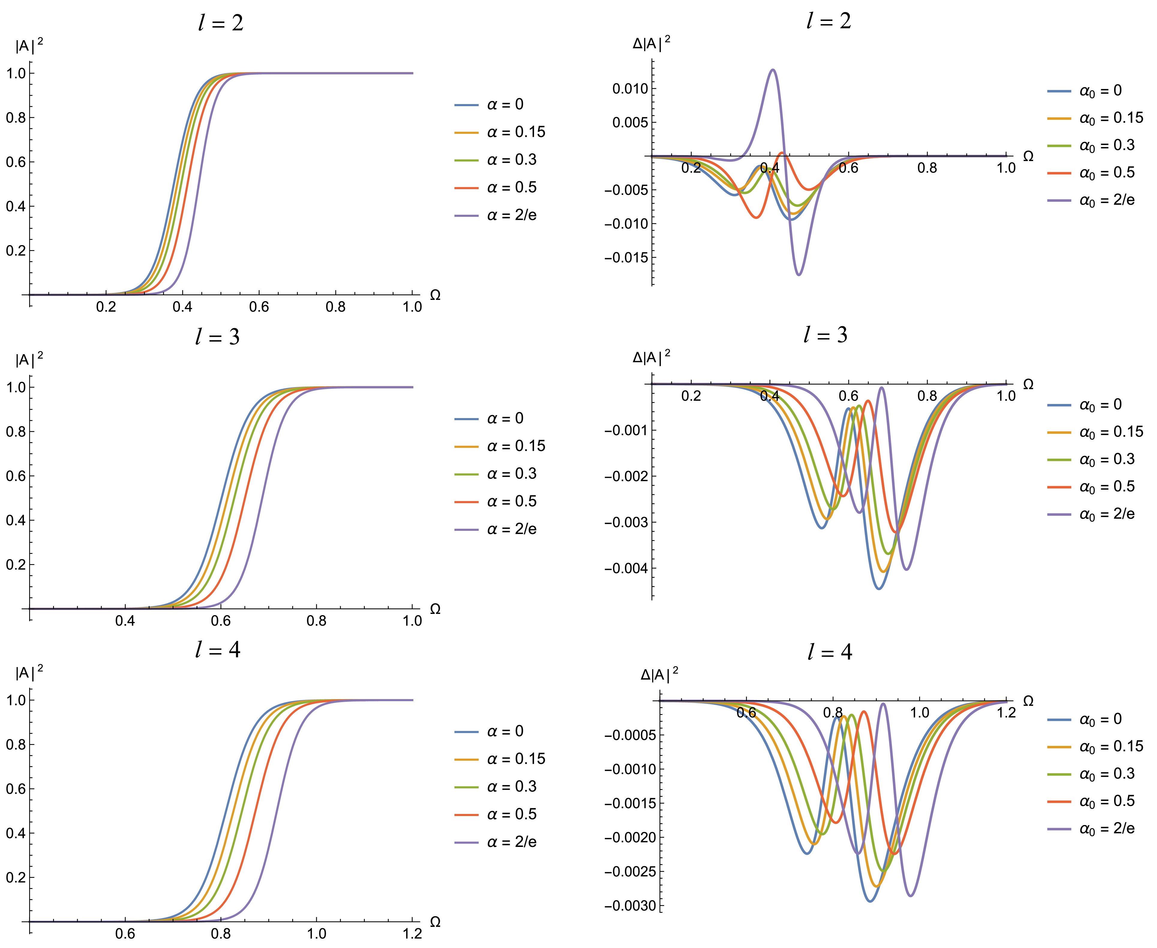
Figure 6. (color online) Left image: Grey-body factors derived from the correspondence of regular black holes with
$ l=2,3,4 $ for different deviation parameters$ \alpha_0 $ . Right image: Discrepancy between the results obtained by the correspondence relation and those obtained by the sixth-order WKB method.• Variation of grey-body factor with Ω: With the increase of the frequency Ω, the grey-body factor gradually increases from 0 to 1. This indicates that they are more likely to penetrate the potential barrier as the energy of the particles becomes larger, thereby resulting in a larger transmission coefficient and an increase in the grey-body factor.
• Variation of grey-body factor with
$ \alpha_0 $ : As the deviation parameter$ \alpha_0 $ increases, the frequency required to achieve the same grey-body factor also increases. This is because an increase in$ \alpha_0 $ leads to a higher effective potential, thereby requiring particles to have a higher frequency to penetrate the barrier.• Difference in grey-body factors: The right plots indicate that the difference between the grey-body factors obtained through the correspondence relation and those obtained using the sixth-order WKB approximation is very small, and this difference exhibits a similar wave-like pattern. As l increases from 2 to 4, the difference between the grey-body factors decreases further, with the discrepancy being only one-thousandth. This further confirms the accuracy of the grey-body factors obtained through the correspondence relation, and it is expected that this correspondence becomes exact in the limit of
$ l\rightarrow \infty $ .To check the universality of this correspondence, we present a brief discussion on other regular black holes with different values of x and c at the end of this section. Without loss of generality, we consider
$ x = 1 $ and$ c = 3 $ . This type of regular black hole has the same asymptotic behavior as the Hayward black hole at large scales. With the same algebra, one can derive that the deviation parameter$ \alpha_0 $ for this regular black hole ranges from 0 to 8/3e. The QNMs of this black hole under the scalar perturbations have been investigated in [41]. We present the QNMs of regular black hole with$ x=1 $ and$ c=3 $ under the gravitational perturbations in Table 5. We list the discrepancy of the grey-body factors obtained by the correspondence relation and the sixth-order WKB method separately, where$ \Delta |A|^2 $ represents the maximal value of the discrepancy as it runs as the function of the frequency Ω. The results show that the correspondence relation is also valid for this regular black hole, and the discrepancy decreases with an increase in the angular number l.$ \alpha_0 $ 

$ l=2 $ 

$ l=3 $ 

$ n=0 $ 

$ n=1 $ 

$ \Delta |A|^2 $ 

$ n=0 $ 

$ n=1 $ 

$ \Delta |A|^2 $ 

0 0.373672-0.088962I 0.346711-0.273915I 0.0094 0.599443 -0.092703I 0.582644-0.281298I 0.0045 0.25 0.373672-0.088962I 0.356405-0.265287I 0.0087 0.607122 -0.090469I 0.591806-0.274238I 0.0041 0.5 0.386371-0.083093I 0.366047-0.254532I 0.0088 0.615229-0.087722I 0.601026-0.265527I 0.0035 0.75 0.393932-0.078508I 0.375307-0.239352I 0.019 0.624505-0.083924I 0.610438-0.25354I 0.0036 8/3e 0.401236-0.072533I 0.379621-0.221364I 0.05 0.63369-0.079133I 0.617221-0.23921I 0.0056 Table 5. QNMs of the regular black hole (
$ x=1,c=3 $ ) under gravitational perturbations for different values of$ \alpha_0 $ , with$ n=0,1 $ and$ l=2,3 $ . The grey-body factors are obtained by the correspondence relation and the sixth-order WKB method separately, with$ \Delta |A|^2 $ represents the maximal value of the discrepancy as it runs as the function of the frequency Ω. -
In this section we turn to the grey-body factor of this sort of regular black holes. We will compute it with the use of the sixth-order WKB method and then compare the results obtained via the correspondence relation between the QNMs and the grey-body factor. We will focus on the regular black hole with (
$ x=2/3 $ ,$ c=2 $ ), and then present a brief discussion on the other regular black holes with different values of x and c.The grey-body factor scattering has the following boundary conditions:
$ \begin{split} &\Phi=Te^{-i\Omega r_{*}} ,\quad r_{*}\to-\infty ,\\&\Phi=e^{-i\Omega r_{*}}+Re^{i\Omega r_{*}} ,\quad r_{*}\to\infty, \end{split} $
(11) where T is the transmission coefficient and R is the reflection coefficient. Here, Ω is a real number, in contrast to QNMs, which have complex frequencies. According to normalization, the transmission coefficient T and the reflection coefficient R are related by the following equation:
$ \begin{split} |T|^2+|R|^2=1. \end{split} $
(12) The reflection coefficient R is approximately calculated using the WKB method as follows:
$ \begin{split} R=(1+e^{-2i\pi{\cal{K}}})^{-1/2}, \end{split} $
(13) where
$ {\cal{K}} $ is determined by the following formula:$ \begin{aligned} {\cal{K}}=i\frac{\omega^2-V_0}{\sqrt{-2V_2}}-\sum_{k=2}^{k=6}\Lambda_k({\cal{K}}), \end{aligned} $
(14) where
$ \Lambda_k({\cal{K}}) $ is the higher WKB corrections [75−77]. Thus, the grey-body factor for different values of l is calculated as:$ \begin{split} |A_l|^2=1-|R|^2=|T|^2. \end{split} $
(15) The correspondence between the QNMs and the grey-body factor has been established in [1], and it is described by an analytical expansion in terms of the angular number l with the following form:
$ \begin{split} \begin{aligned} i{\cal{K}} =\;&\frac{\Omega^2-Re(\omega_0)^2}{4Re(\omega_0)Im(\omega_0)}\left(1+\frac{(Re(\omega_0)-Re(\omega_1))^2}{32Im(\omega_0)^2}-\frac{3Im(\omega_0)-Im(\omega_1)}{24Im(\omega_0)}\right) -\frac{Re(\omega_0)-Re(\omega_1)}{16Im(\omega_0)}\\ &-\frac{(\omega^2-Re(\omega_0)^2)^2}{16Re(\omega_0)^3Im(\omega_0)}\left(1+\frac{Re(\omega_0)(Re(\omega_0)-Re(\omega_1))}{4Im(\omega_0)^2}\right)\\ & +\frac{(\omega^2-Re(\omega_0)^2)^3}{32Re(\omega_0)^5Im(\omega_0)}\left(1+\frac{Re(\omega_0)(Re(\omega_0)-Re(\omega_1))}{4Im(\omega_0)^2}\right. +Re(\omega_0)^2\left(\frac{(Re(\omega_0)-Re(\omega_1))^2}{16Im(\omega_0)^4}-\left.\frac{3Im(\omega_0)-Im(\omega_1)}{12Im(\omega_0)}\right)\right)+{\cal{O}}\left(\frac{1}{\ell^3}\right), \end{aligned} \end{split} $
(16) where Ω represents the frequency of the grey-body factor, while
$ \omega_0 $ and$ \omega_1 $ denote the fundamental mode and the first overtone mode of the QNMs, respectively.Now we intend to check this correspondence for the regular black holes with
$ x=2/3 $ and$ c=2 $ . Fig. 6 illustrates the grey-body factor as the function of the frequency Ω and the difference between the grey-body factors obtained through the correspondence relation and those obtained using the sixth-order WKB method. From these figures, we have following observations and remarks:
Figure 6. Left image: the grey-body factors derived from the correspondence of regular black holes with
$ l=2,3,4 $ for different deviation parameters$ \alpha_0 $ . Right image: the discrepancy between the results by the correspondence relation and those by sixth-order WKB method.• Regarding the variation of grey-body factor with Ω: With the increase of the frequency Ω, the grey-body factor gradually increases from 0 to 1. This indicates that as the energy of particles becomes larger, they are more likely to penetrate the potential barrier, resulting in a larger transmission coefficient and thus an increase in the grey-body factor.
• Regarding the variation of grey-body factor with
$ \alpha_0 $ : As the deviation parameter$ \alpha_0 $ increases, the frequency required to achieve the same grey-body factor also increases. This is because an increase in$ \alpha_0 $ leads to a higher effective potential, requiring particles to have a higher frequency to penetrate the barrier.• Regarding the difference in grey-body factors: From the right plots, it can be seen that the difference between the grey-body factors obtained through the correspondence relation and those obtained using the sixth-order WKB approximation is very small, and this difference exhibits a similar wave-like pattern. Notably, as l increases from 2 to 4, the difference between the grey-body factors further decreases, with the discrepancy being only one-thousandth. This further confirms the accuracy of the grey-body factors obtained through the correspondence relation, and it is expected that this correspondence becomes exact in the limit of
$ l\rightarrow \infty $ .To check the universality of this correspondence, we present a brief discussion on other regular black holes with different values of x and c in the end of this section. Without loss of generality, we consider
$ x = 1 $ and$ c = 3 $ . This type of regular black hole has the same asymptotic behavior as the Hayward black hole at large scales. With the same algebra, one can derive that the deviation parameter$ \alpha_0 $ for this regular black hole ranges from 0 to 8/3e. The QNMs of this black hole under the scalar perturbations were investigated in [42]. Here we present the QNMs of regular black hole with$ x=1 $ and$ c=3 $ under the gravitational perturbations in Table 5. In particular, we list the discrepancy of the grey-body factors obtained by the correspondence relation and the sixth-order WKB method separately, where$ \Delta |A|^2 $ denotes the maximal value of the discrepancy as it runs as the function of the frequency Ω. The results show that the correspondence relation is also valid for this regular black hole, and the discrepancy decreases as the angular number l increases.$ l=2 $ $ l=3 $ $ \alpha_0 $ $ n=0 $ $ n=1 $ $ \Delta |A|^2 $ $ n=0 $ $ n=1 $ $ \Delta |A|^2 $ 0 0.373672-0.088962I 0.346711-0.273915I 0.0094 0.599443 -0.092703I 0.582644-0.281298I 0.0045 0.25 0.373672-0.088962I 0.356405-0.265287I 0.0087 0.607122 -0.090469I 0.591806-0.274238I 0.0041 0.5 0.386371-0.083093I 0.366047-0.254532I 0.0088 0.615229-0.087722I 0.601026-0.265527I 0.0035 0.75 0.393932-0.078508I 0.375307-0.239352I 0.019 0.624505-0.083924I 0.610438-0.25354I 0.0036 8fanxiexian_myfhe 0.401236-0.072533I 0.379621-0.221364I 0.05 0.63369-0.079133I 0.617221-0.23921I 0.0056 Table 5. The QNMs of regular black hole (
$ x=1,c=3 $ ) under gravitational perturbations for different values of$ \alpha_0 $ , with$ n=0,1 $ and$ l=2,3 $ . The grey-body factors are obtained by the correspondence relation and the sixth-order WKB method separately, with$ \Delta |A|^2 $ denoting the maximal value of the discrepancy as it runs as the function of the frequency Ω. -
In this paper, we have computed the QNMs of regular black holes with sub-Planckian curvature under gravitational perturbations by employing the pseudospectral method and the WKB method. As the overtone number n increases, it is observed that the trajectory of the QNMs with the variation of the deviation parameter
$ \alpha_0 $ exhibits non-monotonic behavior in the frequency plane. In particular, for$ l = 2 $ and$ n = 6,\; 7,\; 8 $ , we clearly observed oscillatory behavior in the real part and mild fluctuations in the imaginary part, which are associated with the emergence of spiral structures in the complex frequency plane. For$ l = 3 $ , such behavior does not appear up to$ n = 8 $ , but it is expected to emerge at larger n. Thus, we suggest that the increase of the angular number l might suppress the non-monotonic and spiral behavior of the QNMs on the frequency plane, but further investigation with larger values of l is needed to confirm this suggestion. On the other hand, it is more likely to observe the non-monotonic behavior and spiral behavior of the frequency for larger overtone number n, leading to the outburst of the overtone. We expect to justify this statement by computing the QNMs for larger n in future.Furthermore, we have computed the grey-body factors with the WKB method and then compared them with the results obtained with the correspondence relation between the QNMs and the grey-body factors. The results indicate that for small l, the grey-body factors derived from the correspondence relation have tiny difference compared to those from the WKB method, and these discrepancy decrease further as the angular number l increases, demonstrating the reliability of this approach for regular black holes with sub-Planckian curvature and Minkowski core.
-
In this study, we computed the QNMs of regular black holes with sub-Planckian curvature under gravitational perturbations by employing the pseudospectral and WKB methods. As the overtone number n increases, it is observed that the trajectory of the QNMs with the variation of the deviation parameter
$ \alpha_0 $ exhibits non-monotonic behavior in the frequency plane. For$ l = 2 $ and$ n = 6,\; 7,\; 8 $ , we clearly observed oscillatory behavior in the real part and mild fluctuations in the imaginary part, which are associated with the emergence of spiral structures in the complex frequency plane. For$ l = 3 $ , such behavior does not appear up to$ n = 8 $ ; however, it is expected to emerge at a larger n. Thus, we suggest that the increase in the angular number l may suppress the non-monotonic and spiral behavior of the QNMs on the frequency plane; however, further investigation with larger values of l is required to confirm this suggestion. It is more likely to observe the non-monotonic behavior and spiral behavior of the frequency for larger overtone number n, which leads to the outburst of the overtone. We expect to justify this statement by computing the QNMs for a larger n in future.Furthermore, we computed the grey-body factors with the WKB method and compared them with the results obtained with the correspondence relation between the QNMs and grey-body factors. The results indicate that for small l, the grey-body factors derived from the correspondence relation have a tiny difference compared to those from the WKB method, and these discrepancy decrease further with an increase in the angular number l, thus demonstrating the reliability of this approach for regular black holes with sub-Planckian curvature and Minkowski core.
-
We are grateful to Guo-ping Li, Kai Li, Wen-bin Pan, Meng-he Wu, and Zhangping Yu for helpful discussions on the QNMs and the relevant numerical methods. We also thank the anonymous referees for their helpful comments.
-
We are grateful to Guo-ping Li, Kai Li, Wen-bin Pan, Meng-he Wu, and Zhangping Yu for helpful discussions on the QNMs and the relevant numerical methods. We also thank the anonymous referees for their helpful comments.
Correspondence between grey-body factors and quasinormal modes for regular black holes with sub-Planckian curvature
- Received Date: 2025-05-08
- Available Online: 2025-12-15
Abstract: We investigate the quasi-normal modes (QNMs) under gravitational field perturbations and grey-body factors for a class of regular black holes with sub-Planckian curvature and Minkowski core. We compute the QNMs with the pseudospectral and WKB methods. The trajectory of the QNMs displays non-monotonic and spiral behavior with changes in the deviation parameter of the regular black hole. Subsequently, we compute the grey-body factors with the WKB method and compare them with the results obtained by the correspondence relation recently revealed in [R. A. Konoplya and A. Zhidenko, JCAP 09, 068 (2024)]. We find that the discrepancy exhibits minor errors, indicating that this relation is effective for computing the grey-body factors of such regular black holes.


 DownLoad: