


 Abstract
 HTML
HTML Reference
 Related
 PDF
PDF


-
Proton radioactivity, discovered as a significant spontaneous decay mode in the study of exotic nuclei beyond the
$ \beta $ -stability line, manifests as single-proton and two-proton (2p) radioactivity. First detected by Jackson et al. during the 1970s in the isomeric state of 53Com [1, 2], it was later independently observed from ground states in 151Lu [3] (by Hofmann) and 147Tm [4] (by Klepper). Following these key findings, numerous proton-emitting radionuclides have been identified. To date, research has characterized over 40 such emitters in ground and isomeric states across the Z=51~83 region. Although proton radioactivity exists in nuclei with Z<50, accurately measuring their extremely short half-lives remains challenging because of current limitations in experimental techniques and detection equipment [5]. The phenomenon of true two-proton radioactivity (requiring$ Q_{\rm{2p}} > $ 0 and$ Q_{\rm{p} } < $ 0, where$ Q_{\rm{p}} $ and$ Q_{\rm{2p}} $ represent the single-proton radioactivity released energy and two-proton radioactivity released energy) was first established theoretically by Zel'dovich and Goldansky in the 1960s [6−8]. It was initially observed experimentally in 45Fe at GSI and GANIL in 2002 [9, 10]. Since then, this decay mode has been found in other neutron-deficient nuclei, specifically 54Zn, 48Ni, 19Mg, and 67Kr [11−14]. Before 2002, the not true 2p radioactivity ($ Q_{\rm{2p}} > $ 0 and$ Q_{\rm{p}} > $ 0) was observed from 6Be, 12O, and 16Ne [15−20]. The exploration of nuclear structure and potential proton drip line [21−26] is anticipated to advance through the discovery of more proton-emitting radionuclides, facilitated by upgrades to experimental facilities and methods. As a valuable tool for investigating nuclear properties such as released energy and half-life, proton radioactivity is becoming an increasingly important topic in the field [27−30].Numerous empirical formulas and theoretical models have been developed to study the half-life of proton radioactivity. In the field of single-proton radioactivity, these include the single-folding model [31, 32], generalized liquid drop model (GLDM) [33], relativistic density functional theory [34], density-dependent M3Y effective interactions [35, 36], phenomenological unified fission model [37, 38], distorted-wave Born approximation [39], universal decay law of proton radioactivity (UDLP) [40], Gamow-like model (GLM) [24, 41], Coulomb and proximity potential model (CPPM) [42], deformed relativistic Hartree-Bogoliubov theory in continuum [43], and triaxial relativistic Hartree-Bogoliubov theory in continuum [44], among others. In the field of two-proton radioactivity, these include the direct decay model [45−49], the simultaneous versus sequential decay model [7, 50], diproton model [8, 51], and three-body model, among others [49, 52−55]. Furthermore, empirical formulas serve as critical analytical tools in two-proton emission studies, and they are predominantly derived from the Geiger-Nuttall (G-N) law [56]. Representative formulations include those proposed by Sreeja et al. [57] and Liu et al. [58].
The GLM, a simple phenomenological model, was initially proposed by Zdeb et al. to study
$ \alpha $ decay [59]. The calculated$ \alpha $ decay half-life of the model showed close agreement with experimental values, prompting its extension to proton radioactivity investigation [41]. In this application, the GLM demonstrated high sensitivity of proton radioactivity half-lives to the external barrier position, emphasizing that accurate potential energy curves are vital in calculations. The GLM represents the external potential via the Coulomb and centrifugal potentials and the internal potential as a square well potential. This method has considerably deeper physical foundations and retains the simplicity of the Viola-Seaborg approach [41]. In 2019, Chen et al. modified the GLM to consider the screening effect of the Coulomb interaction between the emitted proton and daughter nuclei on Hulthen potential [24]. In 2021, Liu et al. [60] applied the GLM to two-proton radioactivity research. Subsequently, in 2022, Zhu et al. [61] investigated two-proton radioactivity using the GLM, considering electrostatic screening effects. More recently, in 2024, Zhang et al. [62] developed the deformed Gamow-like model (D-GLM-zhang) to examine how angular momentum affects the half-life of proton radioactivity. Insights into the final Nilsson configuration, and consequently, valuable information about nuclear shape, are provided by studying the half-life associated with proton radioactivity in deformed nuclei. This paper modified the Coulomb interaction between the emitted proton and daughter nucleus by considering the deformation effect of the daughter nucleus and systematically calculated the half-lives of single-proton and two-proton radioactive nuclei.The remainder of this article is organized as follows: Sec. II discusses the theoretical framework of the computational model in detail, Sec. III presents and discusses the results, and Sec. IV summarizes the findings.
-
Proton radioactivity, discovered as a significant spontaneous decay mode in the study of exotic nuclei beyond the
$ \beta $ -stability line, manifests in two types: single-proton and two-proton (2p) radioactivity. First detected by Jackson and colleagues during the 1970s in the isomeric state of 53Com [1, 2], it was later independently observed from ground states in 151Lu [3] (by Hofmann) and 147Tm [4] (by Klepper). Following these key findings, numerous proton-emitting radionuclides have been identified. To date, research has characterized over forty such emitters in ground and isomeric states across the Z=51~83 region. While proton radioactivity also exists in nuclei with Z<50, accurately measuring their extremely short half-lives remains challenging due to current limitations in experimental techniques and detection equipment [5]. The phenomenon of true two-proton radioactivity (requiring$ Q_{\rm{2p}} > $ 0 and$ Q_{\rm{p} } < $ 0, where$ Q_{\rm{p}} $ and$ Q_{\rm{2p}} $ represent the single-proton radioactivity released energy and two-proton radioactivity released energy) was first established theoretically by Zel'dovich and Goldanskii in the 1960s [6−8]. It was initially observed experimentally in 45Fe at GSI and GANIL in 2002 [9, 10]. Since then, this decay mode has also been found in other neutron-deficient nuclei, specifically 54Zn, 48Ni, 19 Mg, and 67Kr [11−14]. Before 2002, the not true 2p radioactivity($ Q_{\rm{2p}} > $ 0 and$ Q_{\rm{p}} > $ 0) was observed from 6Be, 12O, and 16Ne [15−20]. The exploration of nuclear structure and the potential proton drip line [21−26] is anticipated to advance through the discovery of more proton-emitting radionuclides, facilitated by upgrades to experimental facilities and methods. As a valuable tool for investigating nuclear properties such as released energy and half-life, proton radioactivity is becoming an increasingly important topic in the field [27−30].To study the half-life of proton radioactivity, numerous empirical formulas and theoretical models have been developed. In the field of single-proton radioactivity, these include the single-folding model (SFM) [31, 32], the generalized liquid drop model (GLDM) [33], the relativistic density functional theory (RDFT) [34], the density-dependent M3Y (DDM3Y) effective interactions [35, 36], the phenomenological unified fission model (PUFM) [37, 38], the distorted-wave Born approximation (DWBA) [39], the universal decay law of proton radioactivity (UDLP) [40], the Gamow-like model (GLM) [24, 41], the Coulomb and proximity potential model (CPPM) [42] the deformed relativistic Hartree-Bogoliubov theory in continuum (DRHBc) [43] and the triaxial relativistic Hartree-Bogoliubov theory in continuum (TRHBc) [44], among others. In the field of two-proton radioactivity, these include the direct decay model [45−49], the simultaneous versus sequential decay model [7, 50], the diproton model [8, 51], and the three-body model, among others [49, 52−55]. Furthermore, empirical formulas serve as critical analytical tools in two-proton emission studies, predominantly derived from the Geiger-Nuttall (G-N) law [56]. Representative formulations include those proposed by Sreeja et al [57]. and Liu et al [58].
The GLM, a simple phenomenological model, was initially proposed by Zdeb et al to study
$ \alpha $ decay [67]. The model's calculated$ \alpha $ decay half-life showed close agreement with experimental values, prompting to its extension to proton radioactivity investigation [41]. In this application, the GLM demonstrated high sensitivity of proton radioactivity half-lives to the external barrier position, emphasizing that accurate potential energy curves are vital in calculations. The GLM represents the external potential via the Coulomb and centrifugal potentials and the internal potential as a square well potential. This method has much deeper physical foundations and retains the simplicity of the Viola-Seaborg approach [41]. In 2019, Chen et al modified the GLM to account for the screening effect of the Coulomb interaction between emitted proton and daughter nuclei on Hulthen potential [24]. In 2021, Liu et al [68] applied the GLM to two-proton radioactivity research. Subsequently, in 2022, Zhu et al [69] investigated two-proton radioactivity using the GLM, considering electrostatic screening effects. More recently, in 2024, Zhang et al developed the deformed Gamow-like Model (D-GLM-zhang) [70] to examine how angular momentum impacts the half-life of proton radioactivity. Insights into the final Nilsson configuration and consequently valuable information about nuclear shape—are provided by studying the half-life associated with proton radioactivity in deformed nuclei. This paper modified the Coulomb interaction between the emitted proton and daughter nucleus by considering the deformation effect of the daughter nucleus, and systematically calculated the half-lives of single-proton and two-proton radioactive nuclei.The structure of this article is as follows: Section 2 discusses the theoretical framework of the computational model in detail, Section 3 presents and discusses the results, and Section 4 summarizes the findings.
-
Proton radioactivity, discovered as a significant spontaneous decay mode in the study of exotic nuclei beyond the
$ \beta $ -stability line, manifests as single-proton and two-proton (2p) radioactivity. First detected by Jackson et al. during the 1970s in the isomeric state of 53Com [1, 2], it was later independently observed from ground states in 151Lu [3] (by Hofmann) and 147Tm [4] (by Klepper). Following these key findings, numerous proton-emitting radionuclides have been identified. To date, research has characterized over 40 such emitters in ground and isomeric states across the Z=51~83 region. Although proton radioactivity exists in nuclei with Z<50, accurately measuring their extremely short half-lives remains challenging because of current limitations in experimental techniques and detection equipment [5]. The phenomenon of true two-proton radioactivity (requiring$ Q_{\rm{2p}} > $ 0 and$ Q_{\rm{p} } < $ 0, where$ Q_{\rm{p}} $ and$ Q_{\rm{2p}} $ represent the single-proton radioactivity released energy and two-proton radioactivity released energy) was first established theoretically by Zel'dovich and Goldansky in the 1960s [6−8]. It was initially observed experimentally in 45Fe at GSI and GANIL in 2002 [9, 10]. Since then, this decay mode has been found in other neutron-deficient nuclei, specifically 54Zn, 48Ni, 19Mg, and 67Kr [11−14]. Before 2002, the not true 2p radioactivity ($ Q_{\rm{2p}} > $ 0 and$ Q_{\rm{p}} > $ 0) was observed from 6Be, 12O, and 16Ne [15−20]. The exploration of nuclear structure and potential proton drip line [21−26] is anticipated to advance through the discovery of more proton-emitting radionuclides, facilitated by upgrades to experimental facilities and methods. As a valuable tool for investigating nuclear properties such as released energy and half-life, proton radioactivity is becoming an increasingly important topic in the field [27−30].Numerous empirical formulas and theoretical models have been developed to study the half-life of proton radioactivity. In the field of single-proton radioactivity, these include the single-folding model [31, 32], generalized liquid drop model (GLDM) [33], relativistic density functional theory [34], density-dependent M3Y effective interactions [35, 36], phenomenological unified fission model [37, 38], distorted-wave Born approximation [39], universal decay law of proton radioactivity (UDLP) [40], Gamow-like model (GLM) [24, 41], Coulomb and proximity potential model (CPPM) [42], deformed relativistic Hartree-Bogoliubov theory in continuum [43], and triaxial relativistic Hartree-Bogoliubov theory in continuum [44], among others. In the field of two-proton radioactivity, these include the direct decay model [45−49], the simultaneous versus sequential decay model [7, 50], diproton model [8, 51], and three-body model, among others [49, 52−55]. Furthermore, empirical formulas serve as critical analytical tools in two-proton emission studies, and they are predominantly derived from the Geiger-Nuttall (G-N) law [56]. Representative formulations include those proposed by Sreeja et al. [57] and Liu et al. [58].
The GLM, a simple phenomenological model, was initially proposed by Zdeb et al. to study
$ \alpha $ decay [59]. The calculated$ \alpha $ decay half-life of the model showed close agreement with experimental values, prompting its extension to proton radioactivity investigation [41]. In this application, the GLM demonstrated high sensitivity of proton radioactivity half-lives to the external barrier position, emphasizing that accurate potential energy curves are vital in calculations. The GLM represents the external potential via the Coulomb and centrifugal potentials and the internal potential as a square well potential. This method has considerably deeper physical foundations and retains the simplicity of the Viola-Seaborg approach [41]. In 2019, Chen et al. modified the GLM to consider the screening effect of the Coulomb interaction between the emitted proton and daughter nuclei on Hulthen potential [24]. In 2021, Liu et al. [60] applied the GLM to two-proton radioactivity research. Subsequently, in 2022, Zhu et al. [61] investigated two-proton radioactivity using the GLM, considering electrostatic screening effects. More recently, in 2024, Zhang et al. [62] developed the deformed Gamow-like model (D-GLM-zhang) to examine how angular momentum affects the half-life of proton radioactivity. Insights into the final Nilsson configuration, and consequently, valuable information about nuclear shape, are provided by studying the half-life associated with proton radioactivity in deformed nuclei. This paper modified the Coulomb interaction between the emitted proton and daughter nucleus by considering the deformation effect of the daughter nucleus and systematically calculated the half-lives of single-proton and two-proton radioactive nuclei.The remainder of this article is organized as follows: Sec. II discusses the theoretical framework of the computational model in detail, Sec. III presents and discusses the results, and Sec. IV summarizes the findings.
-
Proton radioactivity, discovered as a significant spontaneous decay mode in the study of exotic nuclei beyond the
$ \beta $ -stability line, manifests as single-proton and two-proton (2p) radioactivity. First detected by Jackson et al. during the 1970s in the isomeric state of 53Com [1, 2], it was later independently observed from ground states in 151Lu [3] (by Hofmann) and 147Tm [4] (by Klepper). Following these key findings, numerous proton-emitting radionuclides have been identified. To date, research has characterized over 40 such emitters in ground and isomeric states across the Z=51~83 region. Although proton radioactivity exists in nuclei with Z<50, accurately measuring their extremely short half-lives remains challenging because of current limitations in experimental techniques and detection equipment [5]. The phenomenon of true two-proton radioactivity (requiring$ Q_{\rm{2p}} > $ 0 and$ Q_{\rm{p} } < $ 0, where$ Q_{\rm{p}} $ and$ Q_{\rm{2p}} $ represent the single-proton radioactivity released energy and two-proton radioactivity released energy) was first established theoretically by Zel'dovich and Goldansky in the 1960s [6−8]. It was initially observed experimentally in 45Fe at GSI and GANIL in 2002 [9, 10]. Since then, this decay mode has been found in other neutron-deficient nuclei, specifically 54Zn, 48Ni, 19Mg, and 67Kr [11−14]. Before 2002, the not true 2p radioactivity ($ Q_{\rm{2p}} > $ 0 and$ Q_{\rm{p}} > $ 0) was observed from 6Be, 12O, and 16Ne [15−20]. The exploration of nuclear structure and potential proton drip line [21−26] is anticipated to advance through the discovery of more proton-emitting radionuclides, facilitated by upgrades to experimental facilities and methods. As a valuable tool for investigating nuclear properties such as released energy and half-life, proton radioactivity is becoming an increasingly important topic in the field [27−30].Numerous empirical formulas and theoretical models have been developed to study the half-life of proton radioactivity. In the field of single-proton radioactivity, these include the single-folding model [31, 32], generalized liquid drop model (GLDM) [33], relativistic density functional theory [34], density-dependent M3Y effective interactions [35, 36], phenomenological unified fission model [37, 38], distorted-wave Born approximation [39], universal decay law of proton radioactivity (UDLP) [40], Gamow-like model (GLM) [24, 41], Coulomb and proximity potential model (CPPM) [42], deformed relativistic Hartree-Bogoliubov theory in continuum [43], and triaxial relativistic Hartree-Bogoliubov theory in continuum [44], among others. In the field of two-proton radioactivity, these include the direct decay model [45−49], the simultaneous versus sequential decay model [7, 50], diproton model [8, 51], and three-body model, among others [49, 52−55]. Furthermore, empirical formulas serve as critical analytical tools in two-proton emission studies, and they are predominantly derived from the Geiger-Nuttall (G-N) law [56]. Representative formulations include those proposed by Sreeja et al. [57] and Liu et al. [58].
The GLM, a simple phenomenological model, was initially proposed by Zdeb et al. to study
$ \alpha $ decay [59]. The calculated$ \alpha $ decay half-life of the model showed close agreement with experimental values, prompting its extension to proton radioactivity investigation [41]. In this application, the GLM demonstrated high sensitivity of proton radioactivity half-lives to the external barrier position, emphasizing that accurate potential energy curves are vital in calculations. The GLM represents the external potential via the Coulomb and centrifugal potentials and the internal potential as a square well potential. This method has considerably deeper physical foundations and retains the simplicity of the Viola-Seaborg approach [41]. In 2019, Chen et al. modified the GLM to consider the screening effect of the Coulomb interaction between the emitted proton and daughter nuclei on Hulthen potential [24]. In 2021, Liu et al. [60] applied the GLM to two-proton radioactivity research. Subsequently, in 2022, Zhu et al. [61] investigated two-proton radioactivity using the GLM, considering electrostatic screening effects. More recently, in 2024, Zhang et al. [62] developed the deformed Gamow-like model (D-GLM-zhang) to examine how angular momentum affects the half-life of proton radioactivity. Insights into the final Nilsson configuration, and consequently, valuable information about nuclear shape, are provided by studying the half-life associated with proton radioactivity in deformed nuclei. This paper modified the Coulomb interaction between the emitted proton and daughter nucleus by considering the deformation effect of the daughter nucleus and systematically calculated the half-lives of single-proton and two-proton radioactive nuclei.The remainder of this article is organized as follows: Sec. II discusses the theoretical framework of the computational model in detail, Sec. III presents and discusses the results, and Sec. IV summarizes the findings.
-
In the DGLM model, the half-life and decay constant of the proton radioactivity are related as
$ T_{1/2}=\frac{\ln 2}{\lambda _{\rm{p/2p}}}, $
(1) where the decay constant
$ \lambda _{\rm{p/2p}} $ is defined as$ \lambda _{\rm{p/2p}}=S_{\rm{p/2p}}\nu P. $
(2) where
$ S_{\rm{p/2p}} $ represents the spectroscopic factor for either single-proton or two-proton radioactive systems,$ P $ represents the barrier penetration probability of the proton, and$ \nu $ represents its collision frequency with the potential barrier.When deformation effects are considered, the radius
$ R_{\rm{in}} $ and Coulomb potential$ V_{\rm{c}} $ of the square well change. Consequently, the total penetration probability is calculated by averaging over all directions as$ P=\frac{1}{2}\int_{0}^{\pi }P_{\theta }\sin \theta \,{\rm d}\theta, $
(3) where
$ \theta $ represents the angle between the subnucleus symmetry axis and radial vector. Under the classical Wentzel-Kramers-Brillouin approximation, this directional penetration probability takes the form$ P_{\theta }=\exp \left[ -\frac{2}{\hbar }\int_{R_{\rm{in}}(\theta )}^{R_{ \mathrm{out}}(\theta )}\sqrt{2\mu |V(r,\theta )-E_{k}|}\,{\rm d}r\right], $
(4) where
$ R_{\rm{in}}(\theta ) $ and$ R_{\rm{out}}(\theta ) $ represent the positions of the inner and outer barriers, respectively. The position$ R_{\rm{out}} $ of the outer barrier is derived from the equation$ V(R_{\rm{out}}(\theta ))=E_{k} $ .$ \mu =\frac{m_{\rm{p/2p}}m_{\rm{d}}}{m_{\rm{p/2p}}+m_{\rm{d}}}\approx 938.3\times A_{\rm{p/2p}}\times \frac{A_{\rm{d}}}{A} \text{ MeV/c}^{2} $ represents the reduced mass, where$ m_{\rm{p/2p}} $ and$ m_{\rm{d}} $ represent the masses of the emitted proton and daughter nuclei, respectively. Further,$ A_{\rm{p/2p}} $ ,$ A_{\rm{d}} $ , and$ A $ represent the mass numbers of the emitted proton, daughter nuclei, and proton emitter, respectively. In addition,$ E_{k}= Q_{\rm{p/2p}}(A- A_{\rm{p/2p}})/A $ represents the kinetic energy of the emitted proton. Incorporating electrostatic screening modifies$ Q_{\rm{p/2p}} $ , which is given by$ Q_{\rm{p/2p}}=\Delta M-(\Delta M_{\rm{d}}+\Delta M_{\rm{p/2p} })+k(Z^{\varepsilon }-Z_{\rm{d}}^{\varepsilon }), $
(5) where Z and
$ Z_{\rm{d}} $ represent the number of protons in the parent and daughter nuclei, respectively.$ \Delta M $ ,$ \Delta M_{\rm{d}} $ , and$ \Delta M_{\rm{p/2p}} $ represent the mass excesses of the parent nucleus, daughter nucleus, and emitted proton, respectively. The term$ k(Z^{\varepsilon }-Z_{\rm{d}}^{\varepsilon }) $ represents the charge screening effect where$ k=8.7$ eV,$ \varepsilon =2.517 $ for$ Z\geq 60 $ and$ k=13.6$ eV,$ \varepsilon =2.408 $ for$ Z<60 $ [63, 64].Summing the daughter nucleus radius and emitted proton radius yields the internal barrier position
$ R_{\rm{in}}(\theta ) $ .$ R_{\rm{in}}(\theta )=R_{\rm{p/2p}}+R_{\rm{d}}(\theta ), $
(6) $ R_{\rm{p/2p}}=r_{0}A_{\rm{p/2p}}^{1/3} $ represents the radius of the emitted proton, where$ A_{\rm{p/2p}} $ represents the mass number of the emitted proton.$ r_{0} $ represents the effective nuclear radius constant and is the only adjustable parameter in this model. Considering the effect of the deformation of the daughter nucleus, the radius is expressed as$ R_{\rm{d}}(\theta )=r_{0}A_{\rm{d}}^{1/3}\left[ 1+\sum\limits_{\lambda }\beta _{\lambda }Y_{\lambda 0}(\theta )\right], $
(7) where
$ \beta _{\lambda } $ represents the deformation parameter of the daughter nucleus ($ \lambda =2,4,6 $ correspond to the quadrupole, hexadecapole, and hexacontatetrapole deformations) and$ \beta _{\lambda } $ values are taken from FRDM2012 [65].$ Y_{\lambda 0}(\theta ) $ represents the spherical harmonics function.The total interaction potential
$ V(r,\theta ) $ between the daughter nucleus and the emitted proton can be expressed as$ V(r,\theta )= \begin{cases} -V_{0}, & 0\leq r\leq R_{\rm{in}}, \\ V_{\rm{c}}(r,\theta )+V_{l}(r), & r>R_{\rm{in}} \end{cases} $
(8) where
$ V_{0} $ represents the depth of the inner square well,$ V_{0}=25A_{\rm{p/2p}}$ MeV [66].$ V_{\rm{c}} $ represents the Coulomb interaction between the daughter nucleus and the emitted proton. Considering the effect of the deformation of the daughter nucleus on the Coulomb potential, the expression for the Coulomb potential is derived as$ \begin{aligned}[b] V_{\rm{c}}(r,\theta ) =\;&\frac{Z_{\rm{d}}Z_{\rm{p/2p}}{\rm{e}}^{2}}{r}+ \frac{3Z_{\rm{d}}Z_{\rm{p/2p}}{\rm{e}}^{2}}{r}\sum\limits_{\lambda =2,4,6}\frac{ 1}{2\lambda +1} \\ & \times \lbrack \frac{R_{\rm{d}}(\theta )}{r}]^{\lambda }Y_{\lambda 0}(\theta )\beta _{\lambda }, \end{aligned} $
(9) where r represents the distance between the daughter nucleus and the emitting proton. The centrifugal potential energy term is expressed as
$ V_{l}(r)=\frac{\hbar ^{2}l(l+1)}{2\mu r^{2}}, $
(10) where l represents the angular momentum carried by the emitted proton and determined by the spin parity conservation law. It can be expressed as [67]
$ l= \begin{cases} \Delta _{j} & {\rm{for\ even}}\; \Delta _{j}\; {\rm{and}}\; \pi =\pi _{\rm{d}}, \\ \Delta _{j}+1 & {\rm{for\ even}}\; \Delta _{j}\; {\rm{and}}\;\pi \neq \pi _{\rm{d}}, \\ \Delta _{j} & {\rm{for\ odd}}\; \Delta _{j}\; {\rm{and}}\; \pi \neq \pi _{\rm{d }}, \\ \Delta _{j}+1 & {\rm{for\ odd}}\; \Delta _{j}\; {\rm{and}}\; \pi =\pi _{\rm{d} }, \end{cases} $
(11) where
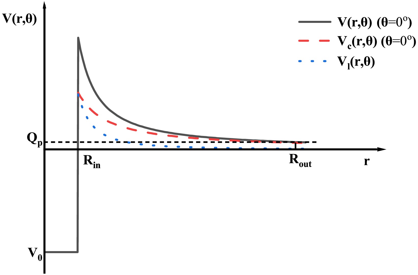
$ \pi $ and$ \pi _{\rm{d}} $ represent the parity of the parent and daughter nuclei, respectively.$ \Delta _{j}=|j-j_{\rm{d}}-j_{\rm{p}}^{\prime }| $ with$ j $ ,$ j_{\rm{d}} $ , and$ j_{\rm{p}}^{\prime } $ being the spins of the parent nucleus and emitted proton (for proton$ j^{\pi }=(1/2)^{+} $ ), respectively. We show the distribution of barriers in Fig. 1. In the first approximation, it is assumed to be given by the harmonic oscillator frequency in the Nilsson potential [68].
Figure 1. (color online) Relationship between the potential energy and center of mass distance of the decay system for 144Tm. The red and blue curves represent the Coulomb potential and centrifugal potential, respectively.
$ h\nu =\hbar \omega \simeq \frac{41}{A^{1/3}}{\rm{MeV}}, $
(12) where
$ h $ ,$ \hbar $ ,$ \omega $ , and$ A $ represent the Planck constant, reduced Planck constant, angular frequency, and mass number of proton emitters, respectively. -
In the DGLM model, proton radioactivity's half-life and decay constant are related as follows:
$ T_{1/2}=\frac{\ln 2}{\lambda _{\rm{p/2p}}}, $

(1) where the decay constant
$ \lambda _{\rm{p/2p}} $ is defined as:$ \lambda _{\rm{p/2p}}=S_{\rm{p/2p}}\nu P. $

(2) Here,
$ S_{\rm{p/2p}} $ represents the spectral factor for either single-proton or two-proton radioactive systems;$ P $ denotes the proton's barrier penetration probability, while$ \nu $ is its collision frequency with the potential barrier.When deformation effects are considered, both the radius
$ R_{\rm{in}} $ and Coulomb potential$ V_{\rm{c}} $ of the square well change. Consequently, the total penetration probability is calculated by averaging over all directions:$ P=\frac{1}{2}\int_{0}^{\pi }P_{\theta }\sin \theta \,d\theta $

(3) where
$ \theta $ denotes the angle between the subnucleus symmetry axis and the radial vector. Under the classical WKB (Wentzel-Kramers-Brillouin) approximation, this directional penetration probability takes the form:$ P_{\theta }=\exp \left[ -\frac{2}{\hbar }\int_{R_{\rm{in}}(\theta )}^{R_{ \mathrm{out}}(\theta )}\sqrt{2\mu |V(r,\theta )-E_{k}|}\,dr\right] $

(4) where
$ R_{\rm{in}}(\theta ) $ and$ R_{\rm{out}}(\theta ) $ are the positions of the inner and outer barriers. The position$ R_{\rm{out}} $ of the outer barrier is derived from the equation$ V(R_{\rm{out}}(\theta ))=E_{k} $ .$ \mu =\frac{m_{\rm{p/2p}}m_{\rm{d}}}{m_{\rm{p/2p}}+m_{\rm{d}}}\approx 938.3\times A_{\rm{p/2p}}\times \frac{A_{\rm{d}}}{A} \text{ MeV/c}^{2} $ is the reduced mass, where$ m_{\rm{p/2p}} $ and$ m_{\rm{d}} $ are the masses of the emitted proton and the daughter nuclei, respectively.$ A_{\rm{p/2p}} $ ,$ A_{\rm{d}} $ , and$ A $ are the mass numbers of the emitted proton, the daughter nuclei, and proton emitter, respectively. In addition,$ E_{k}=Q_{\rm{p/2p}}(A-A_{\rm{p/2p}})/A $ denotes the kinetic energy of emitted proton. Incorporating electrostatic shielding modifies$ Q_{\rm{p/2p}} $ , which is given by:$ Q_{\rm{p/2p}}=\Delta M-(\Delta M_{\rm{d}}+\Delta M_{\rm{p/2p} })+k(Z^{\varepsilon }-Z_{\rm{d}}^{\varepsilon }) $

(5) where Z and
$ Z_{\rm{d}} $ are the number of protons in the parent and daughter nuclei, respectively.$ \Delta M $ ,$ \Delta M_{\rm{d}} $ , and$ \Delta M_{\rm{p/2p}} $ are the mass excesses of the parent nucleus, daughter nucleus, and the emitted proton, respectively. The term$ k(Z^{\varepsilon }-Z_{\rm{d}}^{\varepsilon }) $ denotes the charge shielding effect, where$ k=8.7$ eV,$ \varepsilon =2.517 $ for$ Z\geq 60 $ , and$ k=13.6$ eV,$ \varepsilon =2.408 $ for$ Z<60 $ [71, 72].Summing the daughter nucleus radius and emitted proton radius yields the internal barrier position
$ R_{\rm{in}}(\theta ) $ :$ R_{\rm{in}}(\theta )=R_{\rm{p/2p}}+R_{\rm{d}}(\theta ) $

(6) $ R_{\rm{p/2p}}=r_{0}A_{\rm{p/2p}}^{1/3} $ is the radius of the emitted proton, where$ A_{\rm{p/2p}} $ represents the mass number of the emitted proton.$ r_{0} $ is the effective nuclear radius constant and is the only adjustable parameter in this model. Considering the influence of the deformation of the daughter nucleus, the radius is expressed as:$ R_{\rm{d}}(\theta )=r_{0}A_{\rm{d}}^{1/3}\left[ 1+\sum\limits_{\lambda }\beta _{\lambda }Y_{\lambda 0}(\theta )\right] $

(7) where
$ \beta _{\lambda } $ is the deformation parameter of the daughter nucleus ($ \lambda =2,4,6 $ correspond to the quadrupole, hexadecapole, and hexacontatetrapole deformations) and$ \beta _{\lambda } $ values are taken from FRDM2012 [73].$ Y_{\lambda 0}(\theta ) $ is the spherical harmonics function.The total interaction potential
$ V(r,\theta ) $ between the daughter nucleus and the emitted proton can be expressed as:$ V(r,\theta )= \begin{cases} -V_{0}, & 0\leq r\leq R_{\rm{in}}, \\ V_{\rm{c}}(r,\theta )+V_{l}(r), & r>R_{\rm{in}} \end{cases} $

(8) where
$ V_{0} $ represents the depth of the inner square well,$ V_{0}=25A_{\rm{p/2p}}$ MeV [74].$ V_{\rm{c}} $ denotes the Coulomb interaction between the daughter nucleus and the emitted proton. Taking into account the impact of the deformation of the daughter nucleus on the Coulomb potential, the expression for the Coulomb potential is derived as follows:$ \begin{aligned}[b] V_{\rm{c}}(r,\theta ) =\;&\frac{Z_{\rm{d}}Z_{\rm{p/2p}}{\rm{e}}^{2}}{r}+ \frac{3Z_{\rm{d}}Z_{\rm{p/2p}}{\rm{e}}^{2}}{r}\sum\limits_{\lambda =2,4,6}\frac{ 1}{2\lambda +1} \\ & \times \lbrack \frac{R_{\rm{d}}(\theta )}{r}]^{\lambda }Y_{\lambda 0}(\theta )\beta _{\lambda }, \end{aligned} $

(9) where r is the distance between the daughter nucleus and the emitting proton. The centrifugal potential energy term is expressed as:
$ V_{l}(r)=\frac{\hbar ^{2}l(l+1)}{2\mu r^{2}}, $

(10) where l is the angular momentum carried by the emitted proton, determined by the spin parity conservation law. It can be expressed as [75]:
$ l= \begin{cases} \Delta _{j} & {\rm{for\ even}}\,\Delta _{j}\,{\rm{and}}\,\pi =\pi _{\rm{d}}, \\ \Delta _{j}+1 & {\rm{for\ even}}\,\Delta _{j}\,{\rm{and}}\,\pi \neq \pi _{\rm{d}}, \\ \Delta _{j} & {\rm{for\ odd}}\,\Delta _{j}\,{\rm{and}}\,\pi \neq \pi _{\rm{d }}, \\ \Delta _{j}+1 & {\rm{for\ odd}}\,\Delta _{j}\,{\rm{and}}\,\pi =\pi _{\rm{d} }, \end{cases} $

(11) where
$ \pi $ and$ \pi _{\rm{d}} $ are the parity of the parent and daughter nuclei, respectively.$ \Delta _{j}=|j-j_{\rm{d}}-j_{\rm{p}}^{\prime }| $ with$ j $ ,$ j_{\rm{d}} $ , and$ j_{\rm{p}}^{\prime } $ being the spins of the parent nucleon and the emitted proton (for proton$ j^{\pi }=(1/2)^{+} $ ), respectively. We show the distribution of barriers in Figure 1. In the first approximation, it is assumed to be given by the harmonic oscillator frequency in the Nilsson potential [76]:
Figure 1. (Color online) The relationship between the potential energy and the decay system's center of mass distance for 144Tm. The red and blue curves represent the Coulomb potential and the centrifugal potential, respectively.
$ h\nu =\hbar \omega \simeq \frac{41}{A^{1/3}}{\rm{MeV}}, $

(12) where
$ h $ ,$ \hbar $ ,$ \omega $ , and$ A $ represent the Planck constant, reduced Planck constant, angular frequency, and mass number of proton emitters, respectively. -
In the DGLM model, the half-life and decay constant of the proton radioactivity are related as
$ T_{1/2}=\frac{\ln 2}{\lambda _{\rm{p/2p}}}, $
(1) where the decay constant
$ \lambda _{\rm{p/2p}} $ is defined as$ \lambda _{\rm{p/2p}}=S_{\rm{p/2p}}\nu P. $
(2) where
$ S_{\rm{p/2p}} $ represents the spectroscopic factor for either single-proton or two-proton radioactive systems,$ P $ represents the barrier penetration probability of the proton, and$ \nu $ represents its collision frequency with the potential barrier.When deformation effects are considered, the radius
$ R_{\rm{in}} $ and Coulomb potential$ V_{\rm{c}} $ of the square well change. Consequently, the total penetration probability is calculated by averaging over all directions as$ P=\frac{1}{2}\int_{0}^{\pi }P_{\theta }\sin \theta \,{\rm d}\theta, $
(3) where
$ \theta $ represents the angle between the subnucleus symmetry axis and radial vector. Under the classical Wentzel-Kramers-Brillouin approximation, this directional penetration probability takes the form$ P_{\theta }=\exp \left[ -\frac{2}{\hbar }\int_{R_{\rm{in}}(\theta )}^{R_{ \mathrm{out}}(\theta )}\sqrt{2\mu |V(r,\theta )-E_{k}|}\,{\rm d}r\right], $
(4) where
$ R_{\rm{in}}(\theta ) $ and$ R_{\rm{out}}(\theta ) $ represent the positions of the inner and outer barriers, respectively. The position$ R_{\rm{out}} $ of the outer barrier is derived from the equation$ V(R_{\rm{out}}(\theta ))=E_{k} $ .$ \mu =\frac{m_{\rm{p/2p}}m_{\rm{d}}}{m_{\rm{p/2p}}+m_{\rm{d}}}\approx 938.3\times A_{\rm{p/2p}}\times \frac{A_{\rm{d}}}{A} \text{ MeV/c}^{2} $ represents the reduced mass, where$ m_{\rm{p/2p}} $ and$ m_{\rm{d}} $ represent the masses of the emitted proton and daughter nuclei, respectively. Further,$ A_{\rm{p/2p}} $ ,$ A_{\rm{d}} $ , and$ A $ represent the mass numbers of the emitted proton, daughter nuclei, and proton emitter, respectively. In addition,$ E_{k}= Q_{\rm{p/2p}}(A- A_{\rm{p/2p}})/A $ represents the kinetic energy of the emitted proton. Incorporating electrostatic screening modifies$ Q_{\rm{p/2p}} $ , which is given by$ Q_{\rm{p/2p}}=\Delta M-(\Delta M_{\rm{d}}+\Delta M_{\rm{p/2p} })+k(Z^{\varepsilon }-Z_{\rm{d}}^{\varepsilon }), $
(5) where Z and
$ Z_{\rm{d}} $ represent the number of protons in the parent and daughter nuclei, respectively.$ \Delta M $ ,$ \Delta M_{\rm{d}} $ , and$ \Delta M_{\rm{p/2p}} $ represent the mass excesses of the parent nucleus, daughter nucleus, and emitted proton, respectively. The term$ k(Z^{\varepsilon }-Z_{\rm{d}}^{\varepsilon }) $ represents the charge screening effect where$ k=8.7$ eV,$ \varepsilon =2.517 $ for$ Z\geq 60 $ and$ k=13.6$ eV,$ \varepsilon =2.408 $ for$ Z<60 $ [63, 64].Summing the daughter nucleus radius and emitted proton radius yields the internal barrier position
$ R_{\rm{in}}(\theta ) $ .$ R_{\rm{in}}(\theta )=R_{\rm{p/2p}}+R_{\rm{d}}(\theta ), $
(6) $ R_{\rm{p/2p}}=r_{0}A_{\rm{p/2p}}^{1/3} $ represents the radius of the emitted proton, where$ A_{\rm{p/2p}} $ represents the mass number of the emitted proton.$ r_{0} $ represents the effective nuclear radius constant and is the only adjustable parameter in this model. Considering the effect of the deformation of the daughter nucleus, the radius is expressed as$ R_{\rm{d}}(\theta )=r_{0}A_{\rm{d}}^{1/3}\left[ 1+\sum\limits_{\lambda }\beta _{\lambda }Y_{\lambda 0}(\theta )\right], $
(7) where
$ \beta _{\lambda } $ represents the deformation parameter of the daughter nucleus ($ \lambda =2,4,6 $ correspond to the quadrupole, hexadecapole, and hexacontatetrapole deformations) and$ \beta _{\lambda } $ values are taken from FRDM2012 [65].$ Y_{\lambda 0}(\theta ) $ represents the spherical harmonics function.The total interaction potential
$ V(r,\theta ) $ between the daughter nucleus and the emitted proton can be expressed as$ V(r,\theta )= \begin{cases} -V_{0}, & 0\leq r\leq R_{\rm{in}}, \\ V_{\rm{c}}(r,\theta )+V_{l}(r), & r>R_{\rm{in}} \end{cases} $
(8) where
$ V_{0} $ represents the depth of the inner square well,$ V_{0}=25A_{\rm{p/2p}}$ MeV [66].$ V_{\rm{c}} $ represents the Coulomb interaction between the daughter nucleus and the emitted proton. Considering the effect of the deformation of the daughter nucleus on the Coulomb potential, the expression for the Coulomb potential is derived as$ \begin{aligned}[b] V_{\rm{c}}(r,\theta ) =\;&\frac{Z_{\rm{d}}Z_{\rm{p/2p}}{\rm{e}}^{2}}{r}+ \frac{3Z_{\rm{d}}Z_{\rm{p/2p}}{\rm{e}}^{2}}{r}\sum\limits_{\lambda =2,4,6}\frac{ 1}{2\lambda +1} \\ & \times \lbrack \frac{R_{\rm{d}}(\theta )}{r}]^{\lambda }Y_{\lambda 0}(\theta )\beta _{\lambda }, \end{aligned} $
(9) where r represents the distance between the daughter nucleus and the emitting proton. The centrifugal potential energy term is expressed as
$ V_{l}(r)=\frac{\hbar ^{2}l(l+1)}{2\mu r^{2}}, $
(10) where l represents the angular momentum carried by the emitted proton and determined by the spin parity conservation law. It can be expressed as [67]
$ l= \begin{cases} \Delta _{j} & {\rm{for\ even}}\; \Delta _{j}\; {\rm{and}}\; \pi =\pi _{\rm{d}}, \\ \Delta _{j}+1 & {\rm{for\ even}}\; \Delta _{j}\; {\rm{and}}\;\pi \neq \pi _{\rm{d}}, \\ \Delta _{j} & {\rm{for\ odd}}\; \Delta _{j}\; {\rm{and}}\; \pi \neq \pi _{\rm{d }}, \\ \Delta _{j}+1 & {\rm{for\ odd}}\; \Delta _{j}\; {\rm{and}}\; \pi =\pi _{\rm{d} }, \end{cases} $
(11) where
$ \pi $ and$ \pi _{\rm{d}} $ represent the parity of the parent and daughter nuclei, respectively.$ \Delta _{j}=|j-j_{\rm{d}}-j_{\rm{p}}^{\prime }| $ with$ j $ ,$ j_{\rm{d}} $ , and$ j_{\rm{p}}^{\prime } $ being the spins of the parent nucleus and emitted proton (for proton$ j^{\pi }=(1/2)^{+} $ ), respectively. We show the distribution of barriers in Fig. 1. In the first approximation, it is assumed to be given by the harmonic oscillator frequency in the Nilsson potential [68].
Figure 1. (color online) Relationship between the potential energy and center of mass distance of the decay system for 144Tm. The red and blue curves represent the Coulomb potential and centrifugal potential, respectively.
$ h\nu =\hbar \omega \simeq \frac{41}{A^{1/3}}{\rm{MeV}}, $
(12) where
$ h $ ,$ \hbar $ ,$ \omega $ , and$ A $ represent the Planck constant, reduced Planck constant, angular frequency, and mass number of proton emitters, respectively. -
In the DGLM model, the half-life and decay constant of the proton radioactivity are related as
$ T_{1/2}=\frac{\ln 2}{\lambda _{\rm{p/2p}}}, $
(1) where the decay constant
$ \lambda _{\rm{p/2p}} $ is defined as$ \lambda _{\rm{p/2p}}=S_{\rm{p/2p}}\nu P. $
(2) where
$ S_{\rm{p/2p}} $ represents the spectroscopic factor for either single-proton or two-proton radioactive systems,$ P $ represents the barrier penetration probability of the proton, and$ \nu $ represents its collision frequency with the potential barrier.When deformation effects are considered, the radius
$ R_{\rm{in}} $ and Coulomb potential$ V_{\rm{c}} $ of the square well change. Consequently, the total penetration probability is calculated by averaging over all directions as$ P=\frac{1}{2}\int_{0}^{\pi }P_{\theta }\sin \theta \,{\rm d}\theta, $
(3) where
$ \theta $ represents the angle between the subnucleus symmetry axis and radial vector. Under the classical Wentzel-Kramers-Brillouin approximation, this directional penetration probability takes the form$ P_{\theta }=\exp \left[ -\frac{2}{\hbar }\int_{R_{\rm{in}}(\theta )}^{R_{ \mathrm{out}}(\theta )}\sqrt{2\mu |V(r,\theta )-E_{k}|}\,{\rm d}r\right], $
(4) where
$ R_{\rm{in}}(\theta ) $ and$ R_{\rm{out}}(\theta ) $ represent the positions of the inner and outer barriers, respectively. The position$ R_{\rm{out}} $ of the outer barrier is derived from the equation$ V(R_{\rm{out}}(\theta ))=E_{k} $ .$ \mu =\frac{m_{\rm{p/2p}}m_{\rm{d}}}{m_{\rm{p/2p}}+m_{\rm{d}}}\approx 938.3\times A_{\rm{p/2p}}\times \frac{A_{\rm{d}}}{A} \text{ MeV/c}^{2} $ represents the reduced mass, where$ m_{\rm{p/2p}} $ and$ m_{\rm{d}} $ represent the masses of the emitted proton and daughter nuclei, respectively. Further,$ A_{\rm{p/2p}} $ ,$ A_{\rm{d}} $ , and$ A $ represent the mass numbers of the emitted proton, daughter nuclei, and proton emitter, respectively. In addition,$ E_{k}= Q_{\rm{p/2p}}(A-A_{\rm{p/2p}})/A $ represents the kinetic energy of the emitted proton. Incorporating electrostatic screening modifies$ Q_{\rm{p/2p}} $ , which is given by$ Q_{\rm{p/2p}}=\Delta M-(\Delta M_{\rm{d}}+\Delta M_{\rm{p/2p} })+k(Z^{\varepsilon }-Z_{\rm{d}}^{\varepsilon }), $
(5) where Z and
$ Z_{\rm{d}} $ represent the number of protons in the parent and daughter nuclei, respectively.$ \Delta M $ ,$ \Delta M_{\rm{d}} $ , and$ \Delta M_{\rm{p/2p}} $ represent the mass excesses of the parent nucleus, daughter nucleus, and emitted proton, respectively. The term$ k(Z^{\varepsilon }-Z_{\rm{d}}^{\varepsilon }) $ represents the charge screening effect where$ k=8.7$ eV,$ \varepsilon =2.517 $ for$ Z\geq 60 $ and$ k=13.6$ eV,$ \varepsilon =2.408 $ for$ Z<60 $ [63, 64].Summing the daughter nucleus radius and emitted proton radius yields the internal barrier position
$ R_{\rm{in}}(\theta ) $ .$ R_{\rm{in}}(\theta )=R_{\rm{p/2p}}+R_{\rm{d}}(\theta ), $
(6) $ R_{\rm{p/2p}}=r_{0}A_{\rm{p/2p}}^{1/3} $ represents the radius of the emitted proton, where$ A_{\rm{p/2p}} $ represents the mass number of the emitted proton.$ r_{0} $ represents the effective nuclear radius constant and is the only adjustable parameter in this model. Considering the effect of the deformation of the daughter nucleus, the radius is expressed as$ R_{\rm{d}}(\theta )=r_{0}A_{\rm{d}}^{1/3}\left[ 1+\sum\limits_{\lambda }\beta _{\lambda }Y_{\lambda 0}(\theta )\right], $
(7) where
$ \beta _{\lambda } $ represents the deformation parameter of the daughter nucleus ($ \lambda =2,4,6 $ correspond to the quadrupole, hexadecapole, and hexacontatetrapole deformations) and$ \beta _{\lambda } $ values are taken from FRDM2012 [65].$ Y_{\lambda 0}(\theta ) $ represents the spherical harmonics function.The total interaction potential
$ V(r,\theta ) $ between the daughter nucleus and the emitted proton can be expressed as$ V(r,\theta )= \begin{cases} -V_{0}, & 0\leq r\leq R_{\rm{in}}, \\ V_{\rm{c}}(r,\theta )+V_{l}(r), & r>R_{\rm{in}} \end{cases} $
(8) where
$ V_{0} $ represents the depth of the inner square well,$ V_{0}=25A_{\rm{p/2p}}$ MeV [66].$ V_{\rm{c}} $ represents the Coulomb interaction between the daughter nucleus and the emitted proton. Considering the effect of the deformation of the daughter nucleus on the Coulomb potential, the expression for the Coulomb potential is derived as$ \begin{aligned}[b] V_{\rm{c}}(r,\theta ) =\;&\frac{Z_{\rm{d}}Z_{\rm{p/2p}}{\rm{e}}^{2}}{r}+ \frac{3Z_{\rm{d}}Z_{\rm{p/2p}}{\rm{e}}^{2}}{r}\sum\limits_{\lambda =2,4,6}\frac{ 1}{2\lambda +1} \\ & \times \lbrack \frac{R_{\rm{d}}(\theta )}{r}]^{\lambda }Y_{\lambda 0}(\theta )\beta _{\lambda }, \end{aligned} $
(9) where r represents the distance between the daughter nucleus and the emitting proton. The centrifugal potential energy term is expressed as
$ V_{l}(r)=\frac{\hbar ^{2}l(l+1)}{2\mu r^{2}}, $
(10) where l represents the angular momentum carried by the emitted proton and determined by the spin parity conservation law. It can be expressed as [67]
$ l= \begin{cases} \Delta _{j} & {\rm{for\ even}}\; \Delta _{j}\; {\rm{and}}\; \pi =\pi _{\rm{d}}, \\ \Delta _{j}+1 & {\rm{for\ even}}\; \Delta _{j}\; {\rm{and}}\;\pi \neq \pi _{\rm{d}}, \\ \Delta _{j} & {\rm{for\ odd}}\; \Delta _{j}\; {\rm{and}}\; \pi \neq \pi _{\rm{d }}, \\ \Delta _{j}+1 & {\rm{for\ odd}}\; \Delta _{j}\; {\rm{and}}\; \pi =\pi _{\rm{d} }, \end{cases} $
(11) where
$ \pi $ and$ \pi _{\rm{d}} $ represent the parity of the parent and daughter nuclei, respectively.$ \Delta _{j}=|j-j_{\rm{d}}-j_{\rm{p}}^{\prime }| $ with$ j $ ,$ j_{\rm{d}} $ , and$ j_{\rm{p}}^{\prime } $ being the spins of the parent nucleus and emitted proton (for proton$ j^{\pi }=(1/2)^{+} $ ), respectively. We show the distribution of barriers in Fig. 1. In the first approximation, it is assumed to be given by the harmonic oscillator frequency in the Nilsson potential [68].
Figure 1. (color online) Relationship between the potential energy and center of mass distance of the decay system for 144Tm. The red and blue curves represent the Coulomb potential and centrifugal potential, respectively.
$ h\nu =\hbar \omega \simeq \frac{41}{A^{1/3}}{\rm{MeV}}, $
(12) where
$ h $ ,$ \hbar $ ,$ \omega $ , and$ A $ represent the Planck constant, reduced Planck constant, angular frequency, and mass number of proton emitters, respectively. -
In this study, we calculate the half-lives of two-proton radioactivity for nuclei with atomic numbers Z=4~36 based on the DGLM. In the two-proton (2p) radioactivity, the spectroscopic factor
$ S_{\rm 2p}=G^{2}[A/(A-2)]^{2n}\chi^{2} $ [51]. Here,$ G^{2}=(2n)!/[2^{2n}(n!)^{2}] $ [69], and n represents the average principal proton oscillator quantum number given by$ n\approx(3{Z})^{1/3}-1 $ [70]. In this study,$ \chi^{2} $ =0.0143 according to a previous study by Cui et al. [71]. For a comparative analysis, our calculated radioactivity half-lives were compared with the experimental data as well as predictions from the GLDM [71] and other empirical formulas. All results are compiled in Table 1. In Table 1, the first three columns list the 2p radioactive emitters, 2p radioactivity released energy, and experimental 2p radioactivity half-lives, respectively. The last three columns present the theoretical 2p radioactivity half-lives calculated using the DGLM, GLDM, and empirical formula of Sreeja.Nucleus $ {}^{A}Z $ 

Q2p /MeV $ \log_{10}T_{1/2}(s) $ 

Exp DGLM GLDM [71] Sreeja [57] 6Be 1.371 [15] −20.30 [15] −19.83 −19.37 −21.95 12O 1.638 [20] >−20.20 [20] −18.1 −19.71 −18.47 1.820 [7] −20.94 [7] −18.38 −19.46 −18.79 1.790 [18] −20.10 [18] −18.31 −19.43 −18.74 1.800 [19] −20.12 [19] −18.32 −19.44 −18.76 16Ne 1.330 [7] −20.64 [7] −16.28 −16.45 −15.94 1.400 [17] −20.38 [17] −16.48 −16.63 −16.16 19Mg 0.750 [13] −11.40 [13] −11.50 −11.79 −10.66 45Fe 1.100 [10] −2.40 [10] −2.11 −2.23 −1.25 1.140 [9] −2.07 [9] −2.60 −2.71 −1.66 1.154 [12] −2.55 [12] −2.75 −2.87 −1.80 1.210 [72] −2.42 [72] −3.38 −3.50 −2.34 48Ni 1.290 [73] −2.52 [73] −2.58 −2.62 −1.61 1.350 [12] −2.08 [12] −3.20 −3.24 −2.13 1.310 [74] −2.52 [74] −2.79 −2.83 −1.80 54Zn 1.280 [75] −2.79 [75] −0.95 −0.87 −0.10 1.480 [11] −2.43 [11] −3.01 −2.95 −1.83 67Kr 1.690 [14] −1.70 [14] −0.81 −1.25 0.31 Table 1. 2p proton radioactivity half-lives. The experimental 2p radioactivity half-lives and decay energies were obtained from the literatures.
For a more intuitive comparison, logarithmic differences between the calculated and experimental radioactivity half-lives are presented in Fig. 2. As shown in the figure, the deviations between the calculated and experimental half-lives for true 2p radioactive nuclei fall within one order of magnitude. This indicates that the DGLM successfully reproduces the experimental 2p radioactive half-lives. The standard deviation (
$ \sigma $ ), as defined below, visually illustrates the discrepancy between the modeled half-lives and experimental results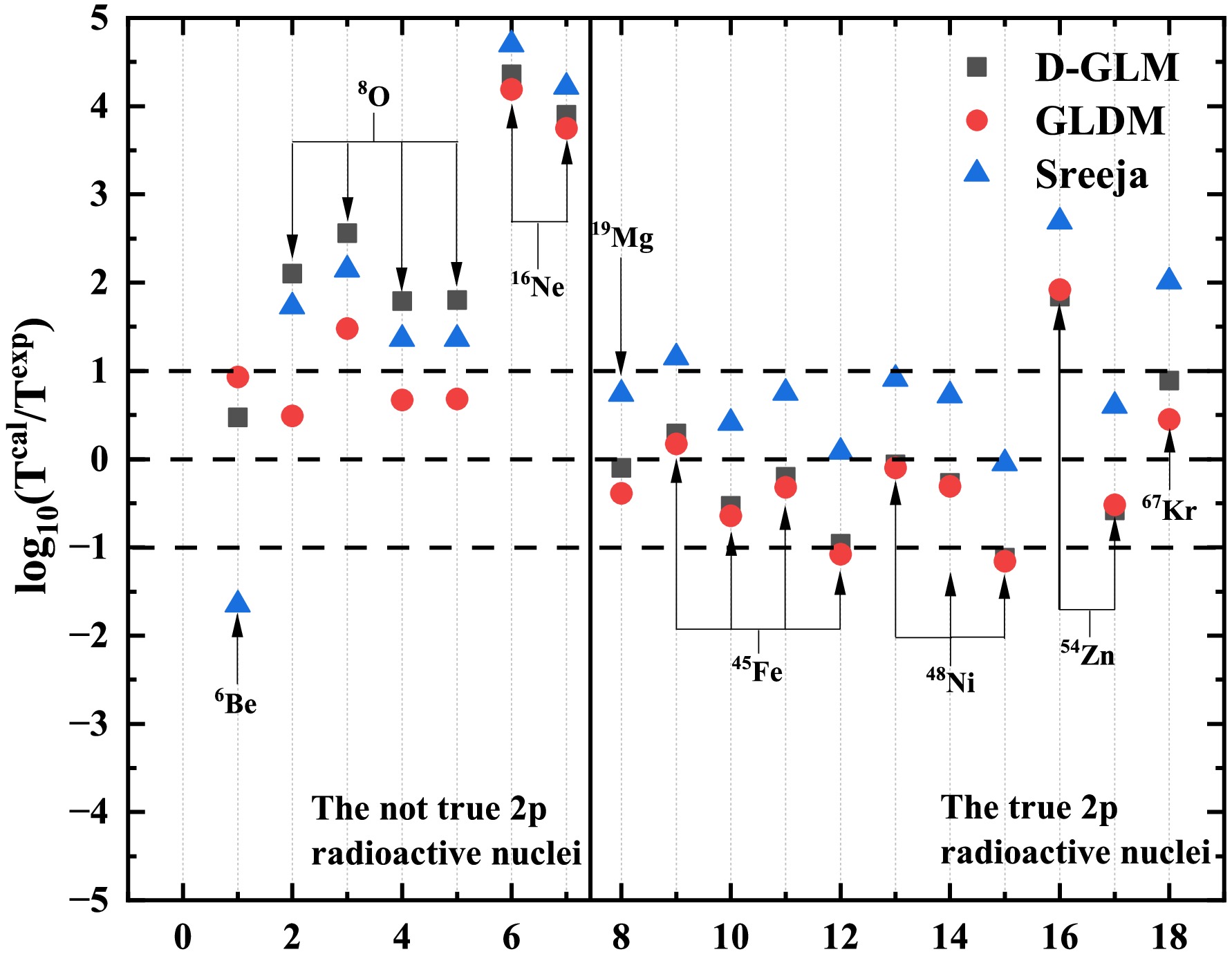
Figure 2. (color online) Discrepancies between calculated and experimental 2p radioactivity half-lives. It encompasses both true 2p radioactivity nuclei and nuclei that do not exhibit true 2p radioactivity.
$ \begin{eqnarray} \sigma = \sqrt{\frac{1}{N}\sum\limits_{i=1}^N \left(\log_{10}T_{\rm{cal}}^i - \log_{10}T_{\rm{exp}}^i\right)^2} \ .\end{eqnarray} $

(13) where
$\log_{10}T_{\rm{cal}}^i$ and$\log_{10}T_{\rm{exp}}^i$ represent the logarithmic values of the calculated and experimental half-lives of 2p radioactivity for the i-th nucleus, respectively. We adjusted the nuclear effective radius and found that when the nuclear effective radius$ r_{0} $ = 1.28 fm, the standard deviation between the experimental half-lives and calculated half-lives was minimized. The effect of the nuclear effective radius on proton radioactivity half-life is shown in Fig. 3, where a minimum point is reached at$ r_{0} $ = 1.28 fm. For true 2p radioactive nuclei, we calculated standard deviations between radioactivity half-lives obtained from the DGLM, GLDM, and Sreeja's empirical formula and the experimental data. The results are presented in Table 2. As show in the table, the standard deviation between the 2p radioactivity half-lives calculated using DGLM and those from experimental data is small. This indicates that the DGLM accurately reproduces the experimental radioactivity half-lives. For short-lived nuclei, the theoretical models fail to reliably reproduce the experimental radioactivity half-lives. This discrepancy may stem from limitations in early detection technologies and radioactive beam facilities, casting doubt on the accuracy of the data.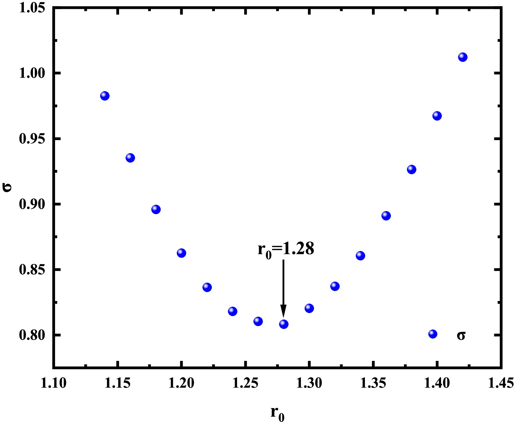
Figure 3. (color online) Dependence of standard deviation between theoretical and experimental half-lives on the effective nuclear radius. Minimal standard deviation is achieved at
$ r_{0} $ = 1.28 fm.DGLM GLDM Sreeja $ \sigma $ 

0.808 0.824 1.191 Table 2. Standard deviations between the experimental half-lives of the true 2p radioactive nuclei and the calculated values using the DGLM, GLDM, and Sreeja's empirical formula, respectively.
Given the successful performance of DGLM in describing 2p radioactivity half-lives, we applied this model to predict the 2p radioactivity half-lives that are energetically permitted but remain unmeasured in NUBASE2020 [76]. For systematic comparison, these predictions were evaluated alongside the results from other theoretical approaches, including ELDM, GLDM, and empirical formula of Sreeja, with all comparative results comprehensively tabulated in Table 3. As shown in Table 3, the 2p radioactivity half-life predictions obtained through DGLM show order-of-magnitude consistency with other theoretical predictions. This consistency highlights the strong predictive capability of DGLM in nuclear decay studies.
Nucleus $ {}^{A}Z $ 

l $ \log_{10}T_{1/2}(s) $ 

DGLM ELDM Sreeja GLDM 22Si 0 −13.292 −13.32 −12.3 −13.3 26S 0 −13.989 −13.86 −12.71 −14.59 34Ca 0 −10.174 −9.91 −8.65 −10.71 38Ti 0 −11.426 −13.56 −11.93 −14.27 39Ti 0 −0.928 −0.81 −0.28 −1.34 42Cr 0 −2.675 −2.43 −1.78 −2.88 49Ni 0 14.559 14.64 12.78 14.46 58Ge 0 −12.352 −11.74 −9.53 −13.1 59Ge 0 −6.317 −5.71 −4.44 −6.97 60Ge 0 14.256 14.62 12.4 13.55 Table 3. Predicted half-lives of 2p proton radioactivity by different models. The spins and parity are obtained from Ref. [76].
-
In this study, we calculate the half-lives of two-proton radioactivity for nuclei with atomic numbers Z=4~36 based on the DGLM. In the two-proton (2p) radioactivity, the spectroscopic factor
$ S_{\rm 2p}=G^{2}[A/(A-2)]^{2n}\chi^{2} $ [51]. Here,$ G^{2}=(2n)!/[2^{2n}(n!)^{2}] $ [69], and n represents the average principal proton oscillator quantum number given by$ n\approx(3{Z})^{1/3}-1 $ [70]. In this study,$ \chi^{2} $ =0.0143 according to a previous study by Cui et al. [71]. For a comparative analysis, our calculated radioactivity half-lives were compared with the experimental data as well as predictions from the GLDM [71] and other empirical formulas. All results are compiled in Table 1. In Table 1, the first three columns list the 2p radioactive emitters, 2p radioactivity released energy, and experimental 2p radioactivity half-lives, respectively. The last three columns present the theoretical 2p radioactivity half-lives calculated using the DGLM, GLDM, and empirical formula of Sreeja.Nucleus $ {}^{A}Z $ Q2p /MeV $ \log_{10}T_{1/2}(s) $ Exp DGLM GLDM [71] Sreeja [57] 6Be 1.371 [15] −20.30 [15] −19.83 −19.37 −21.95 12O 1.638 [20] >−20.20 [20] −18.1 −19.71 −18.47 1.820 [7] −20.94 [7] −18.38 −19.46 −18.79 1.790 [18] −20.10 [18] −18.31 −19.43 −18.74 1.800 [19] −20.12 [19] −18.32 −19.44 −18.76 16Ne 1.330 [7] −20.64 [7] −16.28 −16.45 −15.94 1.400 [17] −20.38 [17] −16.48 −16.63 −16.16 19Mg 0.750 [13] −11.40 [13] −11.50 −11.79 −10.66 45Fe 1.100 [10] −2.40 [10] −2.11 −2.23 −1.25 1.140 [9] −2.07 [9] −2.60 −2.71 −1.66 1.154 [12] −2.55 [12] −2.75 −2.87 −1.80 1.210 [72] −2.42 [72] −3.38 −3.50 −2.34 48Ni 1.290 [73] −2.52 [73] −2.58 −2.62 −1.61 1.350 [12] −2.08 [12] −3.20 −3.24 −2.13 1.310 [74] −2.52 [74] −2.79 −2.83 −1.80 54Zn 1.280 [75] −2.79 [75] −0.95 −0.87 −0.10 1.480 [11] −2.43 [11] −3.01 −2.95 −1.83 67Kr 1.690 [14] −1.70 [14] −0.81 −1.25 0.31 Table 1. 2p proton radioactivity half-lives. The experimental 2p radioactivity half-lives and decay energies were obtained from the literatures.
For a more intuitive comparison, logarithmic differences between the calculated and experimental radioactivity half-lives are presented in Fig. 2. As shown in the figure, the deviations between the calculated and experimental half-lives for true 2p radioactive nuclei fall within one order of magnitude. This indicates that the DGLM successfully reproduces the experimental 2p radioactive half-lives. The standard deviation (
$ \sigma $ ), as defined below, visually illustrates the discrepancy between the modeled half-lives and experimental results
Figure 2. (color online) Discrepancies between calculated and experimental 2p radioactivity half-lives. It encompasses both true 2p radioactivity nuclei and nuclei that do not exhibit true 2p radioactivity.
$ \begin{eqnarray} \sigma = \sqrt{\frac{1}{N}\sum\limits_{i=1}^N \left(\log_{10}T_{\rm{cal}}^i - \log_{10}T_{\rm{exp}}^i\right)^2} \ .\end{eqnarray} $
(13) where
$\log_{10}T_{\rm{cal}}^i$ and$\log_{10}T_{\rm{exp}}^i$ represent the logarithmic values of the calculated and experimental half-lives of 2p radioactivity for the i-th nucleus, respectively. We adjusted the nuclear effective radius and found that when the nuclear effective radius$ r_{0} $ = 1.28 fm, the standard deviation between the experimental half-lives and calculated half-lives was minimized. The effect of the nuclear effective radius on proton radioactivity half-life is shown in Fig. 3, where a minimum point is reached at$ r_{0} $ = 1.28 fm. For true 2p radioactive nuclei, we calculated standard deviations between radioactivity half-lives obtained from the DGLM, GLDM, and Sreeja's empirical formula and the experimental data. The results are presented in Table 2. As show in the table, the standard deviation between the 2p radioactivity half-lives calculated using DGLM and those from experimental data is small. This indicates that the DGLM accurately reproduces the experimental radioactivity half-lives. For short-lived nuclei, the theoretical models fail to reliably reproduce the experimental radioactivity half-lives. This discrepancy may stem from limitations in early detection technologies and radioactive beam facilities, casting doubt on the accuracy of the data.
Figure 3. (color online) Dependence of standard deviation between theoretical and experimental half-lives on the effective nuclear radius. Minimal standard deviation is achieved at
$ r_{0} $ = 1.28 fm.DGLM GLDM Sreeja $ \sigma $ 0.808 0.824 1.191 Table 2. Standard deviations between the experimental half-lives of the true 2p radioactive nuclei and the calculated values using the DGLM, GLDM, and Sreeja's empirical formula, respectively.
Given the successful performance of DGLM in describing 2p radioactivity half-lives, we applied this model to predict the 2p radioactivity half-lives that are energetically permitted but remain unmeasured in NUBASE2020 [76]. For systematic comparison, these predictions were evaluated alongside the results from other theoretical approaches, including ELDM, GLDM, and empirical formula of Sreeja, with all comparative results comprehensively tabulated in Table 3. As shown in Table 3, the 2p radioactivity half-life predictions obtained through DGLM show order-of-magnitude consistency with other theoretical predictions. This consistency highlights the strong predictive capability of DGLM in nuclear decay studies.
Nucleus $ {}^{A}Z $ l $ \log_{10}T_{1/2}(s) $ DGLM ELDM Sreeja GLDM 22Si 0 −13.292 −13.32 −12.3 −13.3 26S 0 −13.989 −13.86 −12.71 −14.59 34Ca 0 −10.174 −9.91 −8.65 −10.71 38Ti 0 −11.426 −13.56 −11.93 −14.27 39Ti 0 −0.928 −0.81 −0.28 −1.34 42Cr 0 −2.675 −2.43 −1.78 −2.88 49Ni 0 14.559 14.64 12.78 14.46 58Ge 0 −12.352 −11.74 −9.53 −13.1 59Ge 0 −6.317 −5.71 −4.44 −6.97 60Ge 0 14.256 14.62 12.4 13.55 Table 3. Predicted half-lives of 2p proton radioactivity by different models. The spins and parity are obtained from Ref. [76].
-
In this work, we calculate half-lives of two-proton radioactivity for nuclei with atomic numbers Z=4~36 based on the DGLM. In the two-proton (2p) radioactivity, the spectroscopic factor
$ S_{\rm 2p}=G^{2}[A/(A-2)]^{2n}\chi^{2} $ [51]. Here$ G^{2}=(2n)!/[2^{2n}(n!)^{2}] $ [77], and n is the average principal proton oscillator quantum number given by$ n\approx(3{Z})^{1/3}-1 $ [78]. In this study,$ \chi^{2} $ =0.0143, according to a previous study by Cui et al. [79]. For comparative analysis, our calculated radioactivity half-lives were compared with the experimental data as well as predictions from the generalized liquid drop model(GLDM) [79] and other empirical formulas. All results are compiled in Table 1. In Table 1, the first three columns list the 2p radioactive emitters, the 2p radioactivity released energy, and the experimental 2p radioactivity half-lives, respectively. The last three columns present the theoretical 2p radioactivity half-lives calculated using the DGLM, the GLDM, and empirical formula of Sreeja.Nucleus $ {}^{A}Z $ Q2p MeV $ \log_{10}T_{1/2}(s) $ Exp DGLM GLDM [79] Sreeja [57] 6Be 1.371 [15] −20.30 [15] −19.83 −19.37 −21.95 12O 1.638 [20] >−20.20 [20] −18.1 −19.71 −18.47 1.820 [7] −20.94 [7] −18.38 −19.46 −18.79 1.790 [18] −20.10 [18] −18.31 −19.43 −18.74 1.800 [19] −20.12 [19] −18.32 −19.44 −18.76 16Ne 1.330 [7] −20.64 [7] −16.28 −16.45 −15.94 1.400 [17] −20.38 [17] −16.48 −16.63 −16.16 19Mg 0.750 [13] −11.40 [13] −11.50 −11.79 −10.66 45Fe 1.100 [10] −2.40 [10] −2.11 −2.23 −1.25 1.140 [9] −2.07 [9] −2.60 −2.71 −1.66 1.154 [12] −2.55 [12] −2.75 −2.87 −1.80 1.210 [80] −2.42 [80] −3.38 −3.50 −2.34 48Ni 1.290 [81] −2.52 [81] −2.58 −2.62 −1.61 1.350 [12] −2.08 [12] −3.20 −3.24 −2.13 1.310 [82] −2.52 [82] −2.79 −2.83 −1.80 54Zn 1.280 [83] −2.79 [83] −0.95 −0.87 −0.10 1.480 [11] −2.43 [11] −3.01 −2.95 −1.83 67Kr 1.690 [14] −1.70 [14] −0.81 −1.25 0.31 Table 1. The 2p proton radioactivity half-lives. The experimental 2p radioactivity half-lives and decay energies were obtained from the literatures.
For a more intuitive comparison, the logarithmic differences between the calculated and experimental radioactivity half-lives are presented in Figure 2. As shown in the figure, the deviations between the calculated and experimental half-lives for true 2p radioactive nuclei fall within one order of magnitude. This indicates that the DGLM successfully reproduces the experimental 2p radioactive half-lives. The standard deviation (
$ \sigma $ ), as defined below, visually illustrates the discrepancy between modeled half-lives and experimental results
Figure 2. (Color online) Discrepancies between calculated and experimental 2p radioactivity half-lives. It encompasses both true 2p radioactivity nuclei and nuclei that do not exhibit true 2p radioactivity.
$ \begin{eqnarray} \sigma = \sqrt{\frac{1}{N}\sum\limits_{i=1}^N \left(\log_{10}T_{\rm{cal}}^i - \log_{10}T_{\rm{exp}}^i\right)^2} \end{eqnarray} $
(13) Here,
$\log_{10}T_{\rm{cal}}^i$ and$\log_{10}T_{\rm{exp}}^i$ represent the logarithmic values of the calculated and experimental half-lives of 2p radioactivity for the i-th nucleus, respectively. We adjusted the nuclear effective radius and found that when the nuclear effective radius$ r_{0} $ = 1.28 fm, the standard deviation between the experimental half-lives and calculated half-lives is minimized. The influence of the nuclear effective radius on proton radioactivity half-life is shown in Figure 3, where a minimum point is reached at$ r_{0} $ = 1.28 fm. For true 2p radioactive nuclei, we calculated the standard deviations between the radioactivity half-lives obtained from the DGLM, GLDM, and Sreeja's empirical formula, and the experimental data. The results are presented in Table 2. As show in the table, the standard deviation between the 2p radioactivity half-lives calculated using DGLM and those from experimental data is small. This indicate that the DGLM accurately reproduces the experimental radioactivity half-lives. It is noteworthy that for short-lived nuclei, the theoretical models fail to reliably reproduce the experimental radioactivity half-lives. This discrepancy may stem from limitations in early detection technologies and radioactive beam facilities, casting doubt on the accuracy of the data.
Figure 3. (Color online) Dependence of the standard deviation between theoretical and experimental half-lives on the effective nuclear radius. Minimal standard deviation is achieved at
$ r_{0} $ =1.28fm.DGLM GLDM Sreeja $ \sigma $ 0.808 0.824 1.191 Table 2. Standard deviations between the experimental half-lives of the true 2p radioactive nuclei and the calculated values using the DGLM, GLDM, and Sreeja, respectively.
Given the DGLM's successful performance in describing 2p radioactivity half-lives, we applied this model to predict the 2p radioactivity half-lives that are energetically permitted but remain unmeasured in NUBASE2020 [86]. For systematic comparison, these predictions were evaluated alongside result form other theoretical approaches, including the ELDM, GLDM, and empirical formula of Sreeja, with all comparative results comprehensively tabulated in Table 3. As shown in Table 3, the 2p radioactivity half-life predictions obtained through DGLM show order-of-magnitude consistency with other theoretical predictions. This consistency highlights the strong predictive capability of DGLM in nuclear decay studies.
Nucleus $ {}^{A}Z $ l $ \log_{10}T_{1/2}(s) $ DGLM ELDM Sreeja GLDM 22Si 0 −13.292 −13.32 −12.3 −13.3 26S 0 −13.989 −13.86 −12.71 −14.59 34Ca 0 −10.174 −9.91 −8.65 −10.71 38Ti 0 −11.426 −13.56 −11.93 −14.27 39Ti 0 −0.928 −0.81 −0.28 −1.34 42Cr 0 −2.675 −2.43 −1.78 −2.88 49Ni 0 14.559 14.64 12.78 14.46 58Ge 0 −12.352 −11.74 −9.53 −13.1 59Ge 0 −6.317 −5.71 −4.44 −6.97 60Ge 0 14.256 14.62 12.4 13.55 Table 3. The predicted half-lives of 2p proton radioactivity by different models. The spins and parity are obtained from Ref. [86].
-
In this study, we calculate the half-lives of two-proton radioactivity for nuclei with atomic numbers Z=4~36 based on the DGLM. In the two-proton (2p) radioactivity, the spectroscopic factor
$ S_{\rm 2p}=G^{2}[A/(A-2)]^{2n}\chi^{2} $ [51]. Here,$ G^{2}=(2n)!/[2^{2n}(n!)^{2}] $ [69], and n represents the average principal proton oscillator quantum number given by$ n\approx(3{Z})^{1/3}-1 $ [70]. In this study,$ \chi^{2} $ =0.0143 according to a previous study by Cui et al. [71]. For a comparative analysis, our calculated radioactivity half-lives were compared with the experimental data as well as predictions from the GLDM [71] and other empirical formulas. All results are compiled in Table 1. In Table 1, the first three columns list the 2p radioactive emitters, 2p radioactivity released energy, and experimental 2p radioactivity half-lives, respectively. The last three columns present the theoretical 2p radioactivity half-lives calculated using the DGLM, GLDM, and empirical formula of Sreeja.Nucleus $ {}^{A}Z $ Q2p /MeV $ \log_{10}T_{1/2}(s) $ Exp DGLM GLDM [71] Sreeja [57] 6Be 1.371 [15] −20.30 [15] −19.83 −19.37 −21.95 12O 1.638 [20] >−20.20 [20] −18.1 −19.71 −18.47 1.820 [7] −20.94 [7] −18.38 −19.46 −18.79 1.790 [18] −20.10 [18] −18.31 −19.43 −18.74 1.800 [19] −20.12 [19] −18.32 −19.44 −18.76 16Ne 1.330 [7] −20.64 [7] −16.28 −16.45 −15.94 1.400 [17] −20.38 [17] −16.48 −16.63 −16.16 19Mg 0.750 [13] −11.40 [13] −11.50 −11.79 −10.66 45Fe 1.100 [10] −2.40 [10] −2.11 −2.23 −1.25 1.140 [9] −2.07 [9] −2.60 −2.71 −1.66 1.154 [12] −2.55 [12] −2.75 −2.87 −1.80 1.210 [72] −2.42 [72] −3.38 −3.50 −2.34 48Ni 1.290 [73] −2.52 [73] −2.58 −2.62 −1.61 1.350 [12] −2.08 [12] −3.20 −3.24 −2.13 1.310 [74] −2.52 [74] −2.79 −2.83 −1.80 54Zn 1.280 [75] −2.79 [75] −0.95 −0.87 −0.10 1.480 [11] −2.43 [11] −3.01 −2.95 −1.83 67Kr 1.690 [14] −1.70 [14] −0.81 −1.25 0.31 Table 1. 2p proton radioactivity half-lives. The experimental 2p radioactivity half-lives and decay energies were obtained from the literatures.
For a more intuitive comparison, logarithmic differences between the calculated and experimental radioactivity half-lives are presented in Fig. 2. As shown in the figure, the deviations between the calculated and experimental half-lives for true 2p radioactive nuclei fall within one order of magnitude. This indicates that the DGLM successfully reproduces the experimental 2p radioactive half-lives. The standard deviation (
$ \sigma $ ), as defined below, visually illustrates the discrepancy between the modeled half-lives and experimental results
Figure 2. (color online) Discrepancies between calculated and experimental 2p radioactivity half-lives. It encompasses both true 2p radioactivity nuclei and nuclei that do not exhibit true 2p radioactivity.
$ \begin{eqnarray} \sigma = \sqrt{\frac{1}{N}\sum\limits_{i=1}^N \left(\log_{10}T_{\rm{cal}}^i - \log_{10}T_{\rm{exp}}^i\right)^2} \ .\end{eqnarray} $
(13) where
$\log_{10}T_{\rm{cal}}^i$ and$\log_{10}T_{\rm{exp}}^i$ represent the logarithmic values of the calculated and experimental half-lives of 2p radioactivity for the i-th nucleus, respectively. We adjusted the nuclear effective radius and found that when the nuclear effective radius$ r_{0} $ = 1.28 fm, the standard deviation between the experimental half-lives and calculated half-lives was minimized. The effect of the nuclear effective radius on proton radioactivity half-life is shown in Fig. 3, where a minimum point is reached at$ r_{0} $ = 1.28 fm. For true 2p radioactive nuclei, we calculated standard deviations between radioactivity half-lives obtained from the DGLM, GLDM, and Sreeja's empirical formula and the experimental data. The results are presented in Table 2. As show in the table, the standard deviation between the 2p radioactivity half-lives calculated using DGLM and those from experimental data is small. This indicates that the DGLM accurately reproduces the experimental radioactivity half-lives. For short-lived nuclei, the theoretical models fail to reliably reproduce the experimental radioactivity half-lives. This discrepancy may stem from limitations in early detection technologies and radioactive beam facilities, casting doubt on the accuracy of the data.
Figure 3. (color online) Dependence of standard deviation between theoretical and experimental half-lives on the effective nuclear radius. Minimal standard deviation is achieved at
$ r_{0} $ = 1.28 fm.DGLM GLDM Sreeja $ \sigma $ 0.808 0.824 1.191 Table 2. Standard deviations between the experimental half-lives of the true 2p radioactive nuclei and the calculated values using the DGLM, GLDM, and Sreeja's empirical formula, respectively.
Given the successful performance of DGLM in describing 2p radioactivity half-lives, we applied this model to predict the 2p radioactivity half-lives that are energetically permitted but remain unmeasured in NUBASE2020 [76]. For systematic comparison, these predictions were evaluated alongside the results from other theoretical approaches, including ELDM, GLDM, and empirical formula of Sreeja, with all comparative results comprehensively tabulated in Table 3. As shown in Table 3, the 2p radioactivity half-life predictions obtained through DGLM show order-of-magnitude consistency with other theoretical predictions. This consistency highlights the strong predictive capability of DGLM in nuclear decay studies.
Nucleus $ {}^{A}Z $ l $ \log_{10}T_{1/2}(s) $ DGLM ELDM Sreeja GLDM 22Si 0 −13.292 −13.32 −12.3 −13.3 26S 0 −13.989 −13.86 −12.71 −14.59 34Ca 0 −10.174 −9.91 −8.65 −10.71 38Ti 0 −11.426 −13.56 −11.93 −14.27 39Ti 0 −0.928 −0.81 −0.28 −1.34 42Cr 0 −2.675 −2.43 −1.78 −2.88 49Ni 0 14.559 14.64 12.78 14.46 58Ge 0 −12.352 −11.74 −9.53 −13.1 59Ge 0 −6.317 −5.71 −4.44 −6.97 60Ge 0 14.256 14.62 12.4 13.55 Table 3. Predicted half-lives of 2p proton radioactivity by different models. The spins and parity are obtained from Ref. [76].
-
Using the improved DGLM, we systematically investigated the half-lives of proton radioactivity in nuclei. Our calculations showed the best agreement with experimental data when using an effective nuclear radius constant of
$ r_{0} $ =1.20 fm, with a standard deviation of 0.527.We performed systematic calculations for nuclei with proton numbers Z=51~83 to study the effect of nuclear deformation on proton radioactivity half-lives. The results are shown in Table 4. Spectroscopic factors
$ S_{\rm{p}} $ were obtained using the relativistic mean field theory plus Bardeen-Cooper-Schrieffer theory (RMF+BCS). According to BCS theory, the spectroscopic factor is given by$ S_{\rm{p}}=u_j^2 $ [77, 78]. In Table 4, the first three columns specify the proton emitter, energy$ Q_{\rm{p}} $ released by the proton, and angular momentum carried by the emitted proton, respectively. The subsequent three columns present the experimental proton radioactivity half-lives, DGLM-calculated proton radioactivity half-lives, and GLM-calculated proton radioactivity half-lives. Comparing these values clearly shows that accounting for nuclear deformation leads to shorter calculated proton radioactivity half-lives.Nucleus $ {}^{A}Z $ 

Qp /MeV l $ \log_{10}T_{1/2}(s) $ 

Exp DGLM GLM 105Sb 0.509 2 2.049 1.612 1.612 108I 0.610 2 0.723 0.619 0.882 109I 0.829 2 −4.032 −4.155 −3.907 112Cs 0.820 2 −3.31 −3.33 −3.065 113Cs 0.981 2 −4.771 −5.513 −5.263 117La 0.831 2 −1.664 −2.456 −2.113 121Pr 0.901 2 −1.921 −2.586 −2.252 130Eu 1.031 2 −3.000 −3.817 −3.489 131Eu 0.963 2 −1.699 −2.914 −2.586 135Tb 1.203 3 −2.996 −4.286 −3.939 140Ho 1.104 3 −2.222 −2.739 −2.417 141Ho 1.194 3 −2.387 −3.79 −3.493 141Hom 1.264 0 −5.137 −6.050 −5.821 144Tm 1.724 5 −5.569 −4.18 −3.817 145Tm 1.754 5 −5.499 −5.67 −5.323 146Tm 0.904 0 −0.81 −0.802 −0.538 146Tmm 1.214 5 −1.137 −1.239 −0.880 147Tm 1.072 5 0.587 0.523 0.846 147Tmm 1.133 2 −3.444 −3.226 −2.972 150Lu 1.285 5 −1.347 −1.247 −0.953 150Lum 1.305 2 −4.398 −4.53 −4.296 151Lu 1.255 5 −0.896 −0.941 −0.651 151Lum 1.315 2 −4.796 −4.647 −4.405 155Ta 1.466 5 −2.495 −2.318 −2.086 156Ta 1.036 2 −0.826 −0.633 −0.405 156Tam 1.126 5 0.933 1.27 1.529 157Ta 0.946 0 −0.527 −0.157 0.070 159Re 1.816 5 −4.678 −4.35 −4.092 159Rem 1.816 5 −4.665 −4.309 −4.051 160Re 1.276 2 −3.163 −3.071 −2.840 161Re 1.216 0 −3.357 −3.303 −3.081 161Rem 1.338 5 −0.678 −0.435 −0.155 164Ir 1.844 5 −3.947 −4.01 −3.742 165Irm 1.727 5 −3.433 −3.222 −2.944 166Ir 1.167 2 −0.824 −0.953 −0.705 166Irm 1.347 5 −0.076 0.032 0.327 167Ir 1.087 0 −1.12 −1.027 −0.791 167Irm 1.262 5 0.842 1.021 1.317 170Au 1.487 2 −3.487 −3.688 −3.414 170Aum 1.767 5 −2.971 −3.24 −2.928 171Au 1.464 0 −4.652 −4.776 −4.569 171Aum 1.718 5 −2.587 −2.327 −2.061 176Tl 1.278 0 −2.208 −1.595 −1.388 177Tl 1.173 0 −1.174 −0.706 −0.491 177Tlm 1.967 5 −3.346 −3.162 −2.913 185Bi 1.598 0 −5.553 −4.809 −4.689 185Bim 1.625 0 −4.191 −3.764 −3.571 Table 4. Single-proton radioactivity half-lives. Symbol m represents the first isomeric state. Experimental data regarding proton emission half-lives, spins, and parity are obtained from Ref. [76]. The released energy is given by Eq. (6), with the exception of the Qp value for 130Eu, 159Re 161Rem, and 164Ir, 177Tlm, and 185Bi, which are taken from Refs. [5, 79].
To further investigate deformation effects, we examined how nuclear deformation affects the penetration probability of proton radioactivity. Employing both the GLM [41] and DGLM with an effective nuclear radius of
$ r_0 = 1.20 $ fm, we calculated the corresponding penetration probabilities. These results are shown in Fig. 4, where the horizontal axis displays the mass number (A) of the proton-emitting nuclei and the vertical axis represents the logarithmic scale of the proton radioactivity penetration probability. Black squares and red circles indicate the penetration probabilities when using the DGLM and GLM, respectively.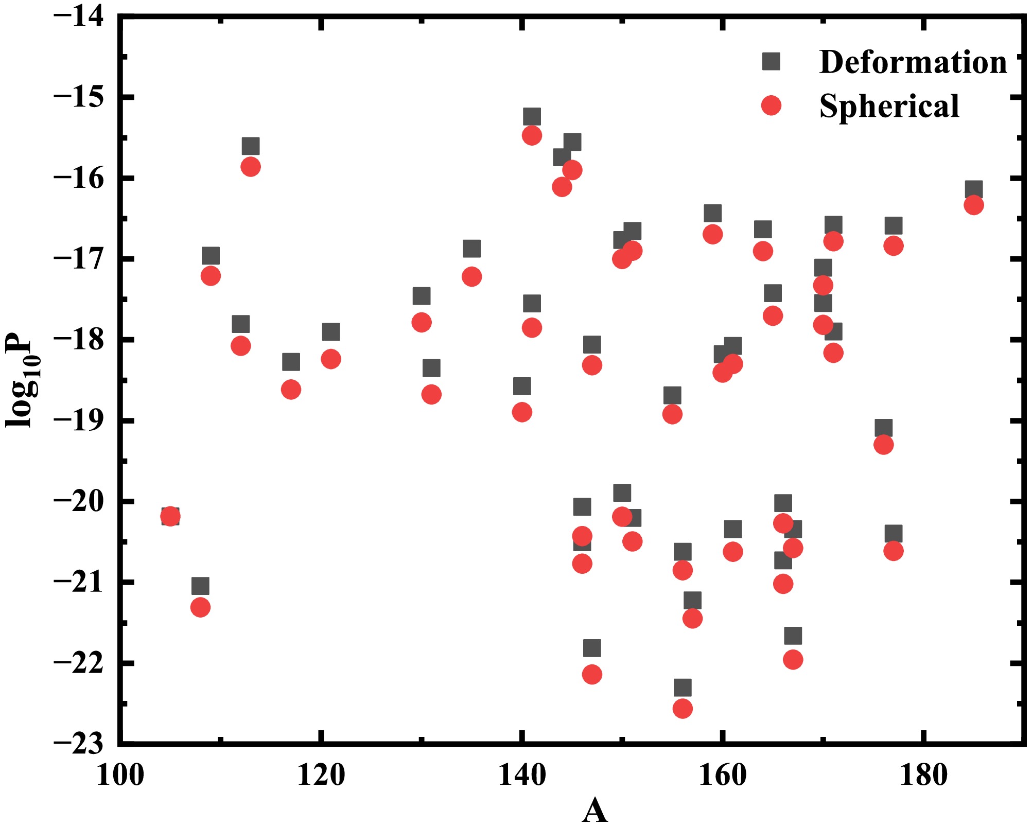
Figure 4. (color online) Penetration probabilities of single-proton radioactivity. The black squares and red circles represent the calculated penetration probabilities with the DGLM and GLM, respectively.
As shown in the figure, differences between penetration probabilities predicted by the DGLM and GLM are small. However, all values from the DGLM are systematically higher than those from the GLM, which indicates that nuclear deformation increases the penetration probability, thereby resulting in a shorter calculated half-life for proton radioactivity.
Subsequently, we investigated the factors affecting the reduction in penetration probability, as well as the effects of deformations in each pole on the potential barrier between the proton and daughter nucleus. Figure 5 shows the distribution of the total interaction potential barrier between the proton and daughter nucleus. In this figure, the black solid, red solid, blue dashed, and green double-dashed lines represent barrier distributions for the undeformed case, quadrupole, hexadecapole, and hexacontatetrapole deformations, respectively. As shown in the figure, nuclear deformation lowers the height and width of the barrier. The height and width of the barrier for the undeformed case are 24.29 MeV and 77.24 fm, respectively, while for the cases with the quadrupole, hexadecapole, and hexacontatetrapole deformations, these values become 23.11 MeV and 77.12 fm, 24.59 MeV and 76.63 fm, and 24.35 MeV and 76.39 fm, respectively. These results indicate that deforming the daughter nucleus reduces both dimensions of the potential barrier, facilitating proton penetration. Notably, quadrupole deformation produces the largest decrease in barrier height.
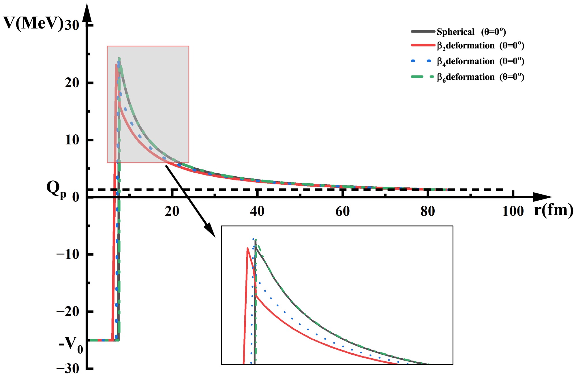
Figure 5. (color online) Total interaction potential between the daughter nucleus and the emitted proton for 150Lu. The black solid, red solid, blue dashed, and green double-dashed lines represent the barrier distributions of the total interaction potential under different conditions: without deformation, with only quadrupole deformation, with only hexadecapole deformation, and with only hexacontatetrapole deformation, respectively.
We computed individual half-lives considering quadrupole, hexadecapole, and hexacontatetrapole deformations to further assess how nuclear deformation affects proton radioactivity half-lives. These results were compared to those from the GLM, as shown in Fig. 6. Our analysis indicates that the calculated half-life decreases with inclusion of deformation effects, with the most significant reduction observed when only quadrupole deformation is considered. For rhenium (Re), the calculated half-life under quadrupole deformation shows the most significant deviation among all. A similar trend is observed for holmium (Ho), lutetium (Lu), and thallium (Tl). These findings confirm that quadrupole deformation plays a pivotal role in reducing proton radioactivity half-lives. This insight deepens our understanding of the nuclear structure of these exotic nuclei.
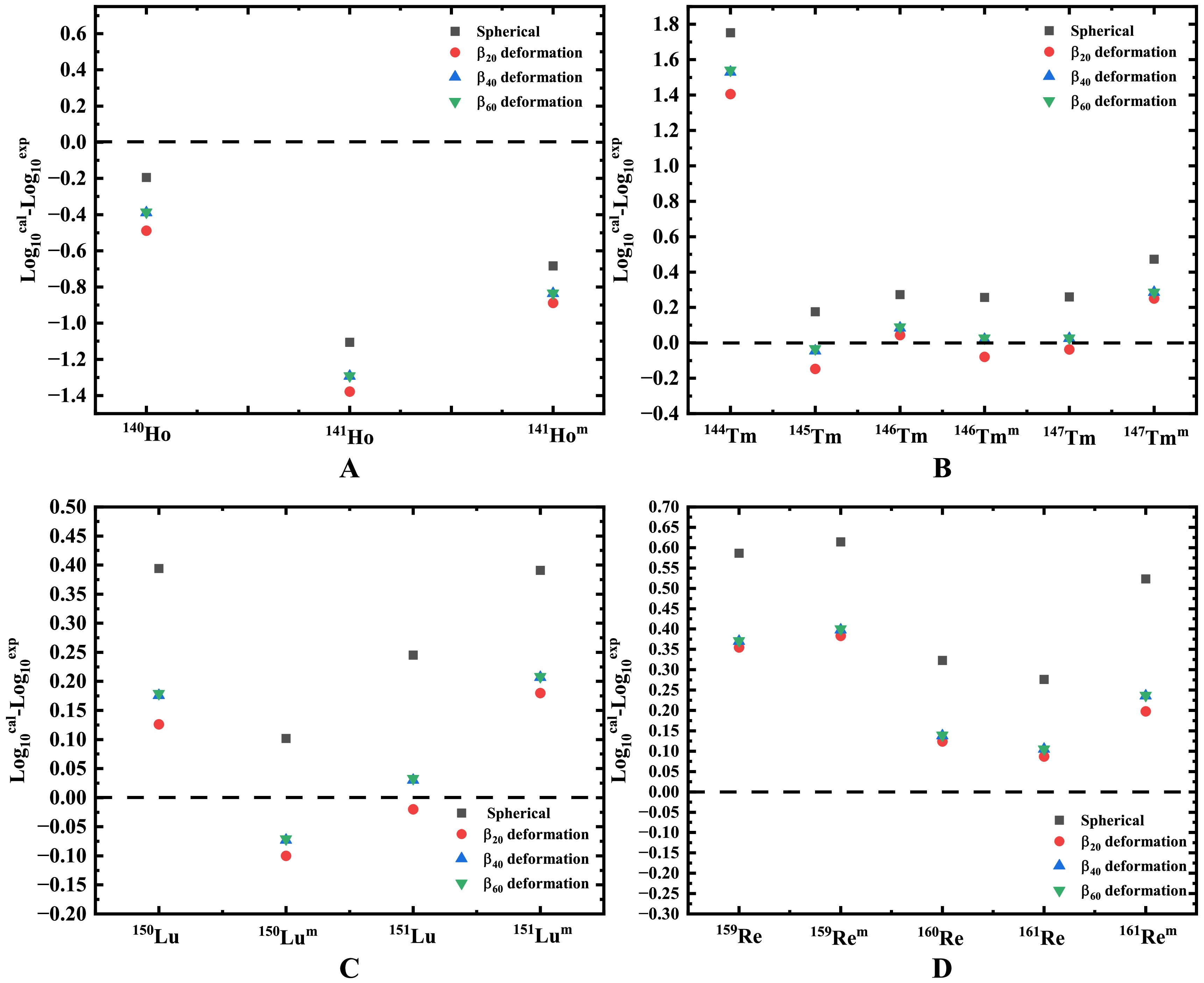
Figure 6. (color online) Half-lives calculated using the DGLM. The red circle, blue square, and green inverted triangle represent the logarithmic forms of the proton radioactivity half-life, calculated individually with DGLM considering quadrupole, hexadecapole, and hexacontatetrapole deformations, respectively. For comparison, the calculation was performed using the GLM, with the results denoted by the black square.
A universal curve exists for
$\alpha$ decay and cluster radioactivity, defined by the negative logarithm of the penetration probability plotted against the logarithm of the experimental half-life. In 2023, Zhang et al. extended this relationship to proton radioactivity, demonstrating its usefulness in evaluating theoretical methods [80]. To better assess the agreement between our model and experimental data, we construct a comparable curve comparing the theoretically predicted half-lives with measured values. Figure 7 illustrates this correlation between$-\log_{10}P$ and$\log_{10}T^{\rm exp}$ . Here, the horizontal axis represents the negative logarithm of the penetration probability calculated for proton radioactivity half-lives using DGLM, while the vertical axis shows the logarithm of the experimental half-life. The strong linear relationship observed between$-\log_{10}P$ and$\log_{10}T^{\rm exp}$ confirms the internal consistency of our computational results.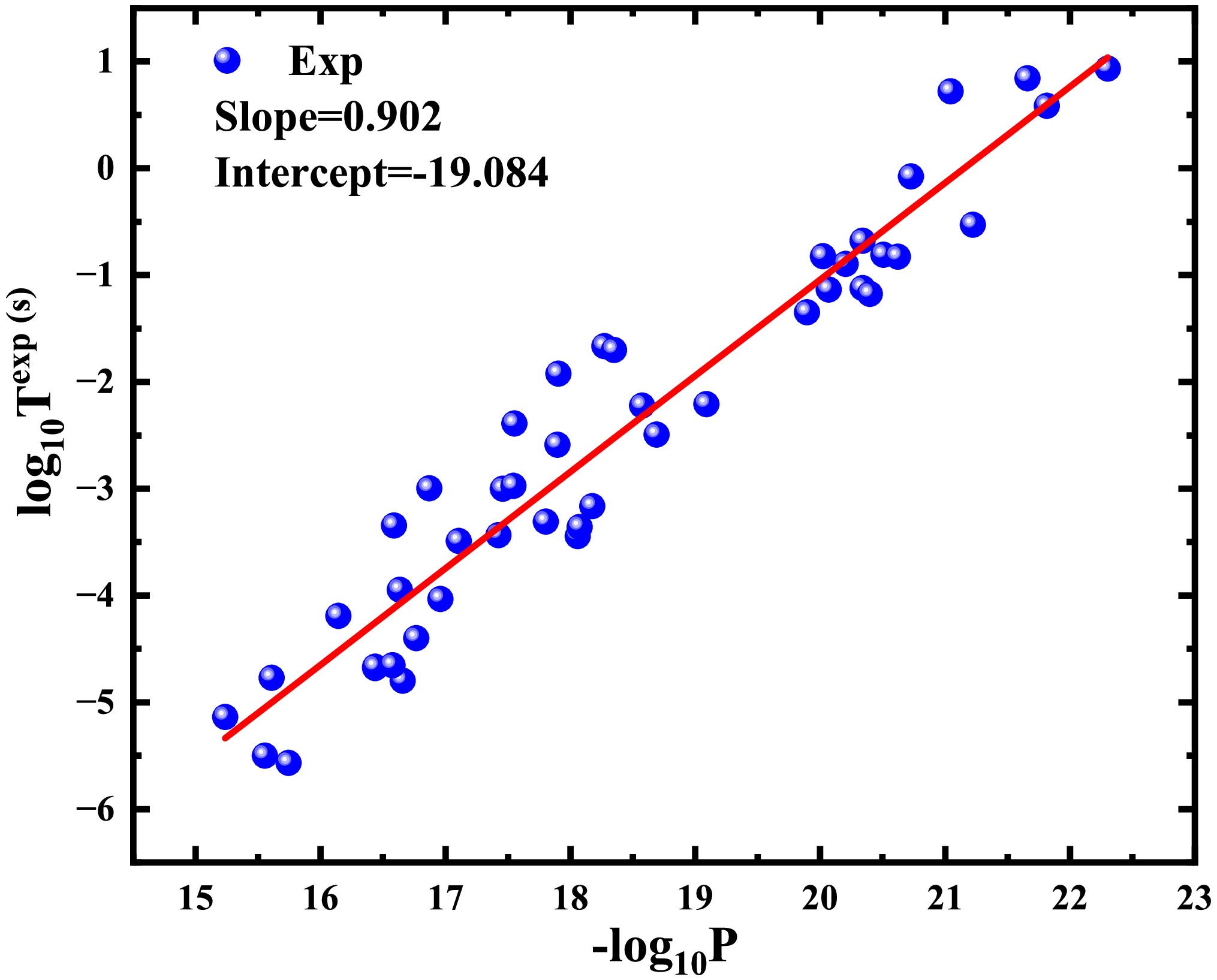
Figure 7. (color online) Universal curve correlating penetration probability with experimental half-life derived using the DGLM.
We thoroughly validated the reliability of our computational model through the systematic calculations of proton radioactivity half-lives. Subsequently, we predicted nuclei within the
$Z=51\sim83$ range to exhibit proton radioactivity, which was unquantified in NUBASE2020 [76]. For comparison, we presented calculations from the unified fission model (UFM) [38], CPPM [42], new Geiger-Nuttall law (NG-N) [24], and UDLP [40] in Table 5. The first two columns of the table show the angular momenta of parent nucleus and emitted proton, while the last five columns list the half-lives of these potential proton radionuclides as calculated by DGLM, UFM, CPPM, NG-N, and UDLP. Significantly, DGLM predictions are comparable in magnitude to the other models, confirming the predictive power of our methodology.Nucleus $ {}^{A}Z $ 

l $ \log_{10}T_{1/2}(s) $ 

DGLM UFM CPPM NG-N UDLP 103Sb 2 −6.545 −6.872 −6.522 −6.009 −5.948 111Cs 2 −10.405 −11.383 −11.229 −10.375 −10.094 116La 2 −8.816 −10.117 −9.963 −9.126 −9.000 165Ir 0 −5.132 −5.791 −5.779 −5.530 −5.387 169Irm 5 9.197 8.799 5.590 8.043 7.362 169Au 0 −7.793 −8.156 −8.249 −7.478 −7.572 172Au 2 4.882 4.357 2.752 3.983 3.578 185Bin 6 −0.385 −0.690 −1.069 −1.512 −1.171 Table 5. Predicted half-lives of single-proton radioactivity by different models. The spins and parity are obtained from Ref. [76]. Here, symbols m and n denote the first and second isomeric states, respectively.
-
Using the improved DGLM, we have systematically investigated the half-lives of proton radioactivity in nuclei. Our calculations show the best agreement with experimental data when using an effective nuclear radius constant of
$ r_{0} $ =1.20 fm, with a standard deviation of 0.527.To study how nuclear deformation influences proton radioactivity half-lives, we performed systematic calculations for nuclei with proton numbers Z=51~83. The results are shown in Table 4. Here the spectroscopic factors
$ S_{\rm{p}} $ were obtained using the relativistic mean field theory plus Bardeen-Cooper-Schriffer theory (RMF+BCS). According to BCS theory, the spectroscopic factor is given by$ S_{\rm{p}}=u_j^2 $ [84, 85]. In the Table 4, the first three columns specify the proton emitter, the energy$ Q_{\rm{p}} $ released by the proton, and the angular momentum carried by the emitted proton, respectively. The subsequent three columns present the experimental proton radioactivity half-lives, the DGLM-calculated proton radioactivity half-lives, and the GLM-calculated proton radioactivity half-lives. Comparing these values clearly shows that accounting for nuclear deformation leads to shorter calculated proton radioactivity half-lives.Nucleus $ {}^{A}Z $ Qp MeV l $ \log_{10}T_{1/2}(s) $ Exp DGLM GLM 105Sb 0.509 2 2.049 1.612 1.612 108I 0.610 2 0.723 0.619 0.882 109I 0.829 2 −4.032 −4.155 −3.907 112Cs 0.820 2 −3.31 −3.33 −3.065 113Cs 0.981 2 −4.771 −5.513 −5.263 117La 0.831 2 −1.664 −2.456 −2.113 121Pr 0.901 2 −1.921 −2.586 −2.252 130Eu 1.031 2 −3.000 −3.817 −3.489 131Eu 0.963 2 −1.699 −2.914 −2.586 135Tb 1.203 3 −2.996 −4.286 −3.939 140Ho 1.104 3 −2.222 −2.739 −2.417 141Ho 1.194 3 −2.387 −3.79 −3.493 141Hom 1.264 0 −5.137 −6.050 −5.821 144Tm 1.724 5 −5.569 −4.18 −3.817 145Tm 1.754 5 −5.499 −5.67 −5.323 146Tm 0.904 0 −0.81 −0.802 −0.538 146Tmm 1.214 5 −1.137 −1.239 −0.880 147Tm 1.072 5 0.587 0.523 0.846 147Tmm 1.133 2 −3.444 −3.226 −2.972 150Lu 1.285 5 −1.347 −1.247 −0.953 150Lum 1.305 2 −4.398 −4.53 −4.296 151Lu 1.255 5 −0.896 −0.941 −0.651 151Lum 1.315 2 −4.796 −4.647 −4.405 155Ta 1.466 5 −2.495 −2.317 −2.086 156Ta 1.036 2 −0.826 −0.633 −0.405 156Tam 1.126 5 0.933 1.27 1.529 157Ta 0.946 0 −0.527 −0.157 0.070 159Re 1.816 5 −4.678 −4.35 −4.092 159Rem 1.816 5 −4.665 −4.309 −4.051 160Re 1.276 2 −3.163 −3.071 −2.840 161Re 1.216 0 −3.357 −3.303 −3.081 161Rem 1.338 5 −0.678 −0.435 −0.155 164Ir 1.844 5 −3.947 −4.01 −3.742 165Irm 1.727 5 −3.433 −3.222 −2.944 166Ir 1.167 2 −0.824 −0.953 −0.705 166Irm 1.347 5 −0.076 0.032 0.327 167Ir 1.087 0 −1.12 −1.027 −0.791 167Irm 1.262 5 0.842 1.021 1.317 170Au 1.487 2 −3.487 −3.688 −3.414 170Aum 1.767 5 −2.971 −3.24 −2.928 171Au 1.464 0 −4.652 −4.776 −4.569 171Aum 1.718 5 −2.587 −2.327 −2.061 176Tl 1.278 0 −2.208 −1.595 −1.388 177Tl 1.173 0 −1.174 −0.706 −0.491 177Tlm 1.967 5 −3.346 −3.162 −2.913 185Bi 1.598 0 −5.553 −4.809 −4.689 185Bim 1.625 0 −4.191 −3.764 −3.571 Table 4. The single-proton radioactivity half-lives. The symbol m represents the first isomeric state. The experimental data regarding proton emission half-lives, spins, and parity are obtained from Ref. [86]. The released energy is given by Eq. 6, with the exception of the Qp value for 130Eu, 159Re 161Rem, and 164Ir, 177Tlm, and185Bi, which are taken from Ref. [5, 87].
To further investigate deformation effects, we examined how nuclear deformation impacts the penetration probability of proton radioactivity. Employing both the GLM [41] and the DGLM with an effective nuclear radius of
$ r_0 = 1.20 $ fm, we calculated the corresponding penetration probabilities. These results are shown in Figure 4, where the horizontal axis displays the mass number (A) of the proton-emitting nuclei and the vertical axis represents the logarithmic scale of the proton radioactivity penetration probability. Black squares and red circles denote the penetration probabilities using the DGLM and GLM, respectively.
Figure 4. (Color online) The penetration probabilities of single-proton radioactivity. The black squares and red circles represent respectively the calculated penetration probabilities with the DGLM and GLM.
As shown in the figure, the differences between penetration probabilities predicted by the DGLM and GLM are small. However, all values from the DGLM are systematically higher than those from the GLM. This indicates that nuclear deformation increases the penetration probability, resulting in a shorter calculated half-life for proton radioactivity.
Subsequently, we investigated the factors influencing the reduction in penetration probability, as well as the effects of deformations in each pole on the potential barrier between the proton and the daughter nucleus. Figure 5 shows the distribution of the total interaction potential barrier between proton and daughter nucleus. In this figure, the black solid line, red solid line, blue dashed line, and green double-dashed line represent the barrier distributions for the undeformed case, the quadrupole, hexadecapole, and hexacontatetrapole deformations, respectively. As shown in the figure, nuclear deformation lowers both the height and width of the barrier. Specifically, the height and width of the barrier for the undeformed case are 24.29 MeV and 77.24 fm, respectively, while for the cases with the quadrupole, hexadecapole, and hexacontatetrapole deformations, these values become 23.11 MeV and 77.12 fm, 24.59 MeV and 76.63 fm, and 24.35 MeV and 76.39 fm, respectively. These results indicate that deforming the daughter nucleus reduces both dimensions of the potential barrier, thereby facilitating proton penetration. Notably, quadrupole deformation produces the largest decrease in barrier height.
Figure 5. (Color online) Shown is the total interaction potential between daughter nucleus and emitted proton for 150Lu. The black solid line, red solid line, blue dashed line, and green double-dashed line represent the barrier distributions of the total interaction potential under different conditions: without deformation, with only quadrupole deformation, with only hexadecapole deformation, and with only hexacontatetrapole deformation, respectively.
To further assess how nuclear deformation affects proton radioactivity half-lives, we computed individual half-lives considering quadrupole, hexadecapole, and hexacontatetrapole deformations. These results were then compared to those from the GLM, as shown in Figure 6. Our analysis indicates that the calculated half-life decreases with the inclusion of deformation effects, with the most significant reduction observed when only quadrupole deformation is considered. For rhenium (Re), the calculated half-life under quadrupole deformation shows the most significant deviation among all. A similar trend is observed for holmium (Ho), lutetium (Lu), and thallium (Tl). These findings confirm that quadrupole deformation plays a pivotal role in reducing proton radioactivity half-lives. This insight deepening our understanding of the nuclear structure of these exotic nuclei.
Figure 6. (Color online) The calculated half-lives using the DGLM. The red circle, blue square, and green inverted triangle represent the logarithmic forms of the proton radioactivity half-life, calculated individually with DGLM considering quadrupole, hexadecapole, and hexacontatetrapole deformations, respectively. For comparison, the calculation was also performed using the GLM, with the results denoted by the black square.
A universal curve exists for
$\alpha$ decay and cluster radioactivity, defined by the negative logarithm of the penetration probability plotted against the logarithm of the experimental half-life. In 2023, Zhang et al extended this relationship to proton radioactivity, demonstrating its usefulness in evaluating theoretical methods [88]. To better assess the agreement between our model and experimental data, we construct a comparable curve comparing the theoretically predicted half-lives with measured values. Figure 7 illustrates this correlation between$-\log_{10}P$ and$\log_{10}T^{exp}$ . Here the horizontal axis represents the negative logarithm of the penetration probability calculated for proton radioactivity half-lives using DGLM, while the vertical axis shows the logarithm of the experimental half-life. The strong linear relationship observed between$-\log_{10}P$ and$\log_{10}T^{exp}$ confirms the internal consistency of our computational results.
Figure 7. (Color online) A universal curve correlating penetration probability with experimental half-life was derived using the DGLM.
Through systematic calculations of proton radioactivity half-lives, we have thoroughly validated the reliability of our computational model. Subsequently, we predict nuclei within the
$Z=51\sim83$ range likely to exhibit proton radioactivity, unquantified in NUBASE2020 [86]. For comparison, we present calculations from the unified fission model(UFM) [38], the Coulomb and proximity potential model(CPPM) [42], the new Geiger-Nuttall law (NG-N) [24], and the universal decay law for proton emission (UDLP) [40] in Table 5. The first two columns of the table show the angular momenta of parent nucleus and emitted proton, while the last five columns list the half-lives of these potential proton radionuclides as calculated by DGLM, UFM, CPPM, NG-N, and UDLP. Significantly, DGLM predictions are comparable in magnitude to other models, confirming the predictive power of our methodology.Nucleus $ {}^{A}Z $ l $ \log_{10}T_{1/2}(s) $ DGLM UFM CPPM NG-N UDLP 103Sb 2 −6.545 −6.872 −6.522 −6.009 −5.948 111Cs 2 −10.405 −11.383 −11.229 −10.375 −10.094 116La 2 −8.816 −10.117 −9.963 −9.126 −9.000 165Ir 0 −5.132 −5.791 −5.779 −5.530 −5.387 169Irm 5 9.197 8.799 5.590 8.043 7.362 169Au 0 −7.793 −8.156 −8.249 −7.478 −7.572 172Au 2 4.882 4.357 2.752 3.983 3.578 185Bin 6 −0.385 −0.690 −1.069 −1.512 −1.171 Table 5. The predicted half-lives of single-proton radioactivity by different models. The spins and parity are obtained from Ref. [86]. Here, the symbols m and n denote the first and second isomeric states, respectively.
-
Using the improved DGLM, we systematically investigated the half-lives of proton radioactivity in nuclei. Our calculations showed the best agreement with experimental data when using an effective nuclear radius constant of
$ r_{0} $ =1.20 fm, with a standard deviation of 0.527.We performed systematic calculations for nuclei with proton numbers Z=51~83 to study the effect of nuclear deformation on proton radioactivity half-lives. The results are shown in Table 4. Spectroscopic factors
$ S_{\rm{p}} $ were obtained using the relativistic mean field theory plus Bardeen-Cooper-Schrieffer theory (RMF+BCS). According to BCS theory, the spectroscopic factor is given by$ S_{\rm{p}}=u_j^2 $ [77, 78]. In Table 4, the first three columns specify the proton emitter, energy$ Q_{\rm{p}} $ released by the proton, and angular momentum carried by the emitted proton, respectively. The subsequent three columns present the experimental proton radioactivity half-lives, DGLM-calculated proton radioactivity half-lives, and GLM-calculated proton radioactivity half-lives. Comparing these values clearly shows that accounting for nuclear deformation leads to shorter calculated proton radioactivity half-lives.Nucleus $ {}^{A}Z $ Qp /MeV l $ \log_{10}T_{1/2}(s) $ Exp DGLM GLM 105Sb 0.509 2 2.049 1.612 1.612 108I 0.610 2 0.723 0.619 0.882 109I 0.829 2 −4.032 −4.155 −3.907 112Cs 0.820 2 −3.31 −3.33 −3.065 113Cs 0.981 2 −4.771 −5.513 −5.263 117La 0.831 2 −1.664 −2.456 −2.113 121Pr 0.901 2 −1.921 −2.586 −2.252 130Eu 1.031 2 −3.000 −3.817 −3.489 131Eu 0.963 2 −1.699 −2.914 −2.586 135Tb 1.203 3 −2.996 −4.286 −3.939 140Ho 1.104 3 −2.222 −2.739 −2.417 141Ho 1.194 3 −2.387 −3.79 −3.493 141Hom 1.264 0 −5.137 −6.050 −5.821 144Tm 1.724 5 −5.569 −4.18 −3.817 145Tm 1.754 5 −5.499 −5.67 −5.323 146Tm 0.904 0 −0.81 −0.802 −0.538 146Tmm 1.214 5 −1.137 −1.239 −0.880 147Tm 1.072 5 0.587 0.523 0.846 147Tmm 1.133 2 −3.444 −3.226 −2.972 150Lu 1.285 5 −1.347 −1.247 −0.953 150Lum 1.305 2 −4.398 −4.53 −4.296 151Lu 1.255 5 −0.896 −0.941 −0.651 151Lum 1.315 2 −4.796 −4.647 −4.405 155Ta 1.466 5 −2.495 −2.318 −2.086 156Ta 1.036 2 −0.826 −0.633 −0.405 156Tam 1.126 5 0.933 1.27 1.529 157Ta 0.946 0 −0.527 −0.157 0.070 159Re 1.816 5 −4.678 −4.35 −4.092 159Rem 1.816 5 −4.665 −4.309 −4.051 160Re 1.276 2 −3.163 −3.071 −2.840 161Re 1.216 0 −3.357 −3.303 −3.081 161Rem 1.338 5 −0.678 −0.435 −0.155 164Ir 1.844 5 −3.947 −4.01 −3.742 165Irm 1.727 5 −3.433 −3.222 −2.944 166Ir 1.167 2 −0.824 −0.953 −0.705 166Irm 1.347 5 −0.076 0.032 0.327 167Ir 1.087 0 −1.12 −1.027 −0.791 167Irm 1.262 5 0.842 1.021 1.317 170Au 1.487 2 −3.487 −3.688 −3.414 170Aum 1.767 5 −2.971 −3.24 −2.928 171Au 1.464 0 −4.652 −4.776 −4.569 171Aum 1.718 5 −2.587 −2.327 −2.061 176Tl 1.278 0 −2.208 −1.595 −1.388 177Tl 1.173 0 −1.174 −0.706 −0.491 177Tlm 1.967 5 −3.346 −3.162 −2.913 185Bi 1.598 0 −5.553 −4.809 −4.689 185Bim 1.625 0 −4.191 −3.764 −3.571 Table 4. Single-proton radioactivity half-lives. Symbol m represents the first isomeric state. Experimental data regarding proton emission half-lives, spins, and parity are obtained from Ref. [76]. The released energy is given by Eq. (6), with the exception of the Qp value for 130Eu, 159Re 161Rem, and 164Ir, 177Tlm, and 185Bi, which are taken from Refs. [5, 79].
To further investigate deformation effects, we examined how nuclear deformation affects the penetration probability of proton radioactivity. Employing both the GLM [41] and DGLM with an effective nuclear radius of
$ r_0 = 1.20 $ fm, we calculated the corresponding penetration probabilities. These results are shown in Fig. 4, where the horizontal axis displays the mass number (A) of the proton-emitting nuclei and the vertical axis represents the logarithmic scale of the proton radioactivity penetration probability. Black squares and red circles indicate the penetration probabilities when using the DGLM and GLM, respectively.
Figure 4. (color online) Penetration probabilities of single-proton radioactivity. The black squares and red circles represent the calculated penetration probabilities with the DGLM and GLM, respectively.
As shown in the figure, differences between penetration probabilities predicted by the DGLM and GLM are small. However, all values from the DGLM are systematically higher than those from the GLM, which indicates that nuclear deformation increases the penetration probability, thereby resulting in a shorter calculated half-life for proton radioactivity.
Subsequently, we investigated the factors affecting the reduction in penetration probability, as well as the effects of deformations in each pole on the potential barrier between the proton and daughter nucleus. Figure 5 shows the distribution of the total interaction potential barrier between the proton and daughter nucleus. In this figure, the black solid, red solid, blue dashed, and green double-dashed lines represent barrier distributions for the undeformed case, quadrupole, hexadecapole, and hexacontatetrapole deformations, respectively. As shown in the figure, nuclear deformation lowers the height and width of the barrier. The height and width of the barrier for the undeformed case are 24.29 MeV and 77.24 fm, respectively, while for the cases with the quadrupole, hexadecapole, and hexacontatetrapole deformations, these values become 23.11 MeV and 77.12 fm, 24.59 MeV and 76.63 fm, and 24.35 MeV and 76.39 fm, respectively. These results indicate that deforming the daughter nucleus reduces both dimensions of the potential barrier, facilitating proton penetration. Notably, quadrupole deformation produces the largest decrease in barrier height.
Figure 5. (color online) Total interaction potential between the daughter nucleus and the emitted proton for 150Lu. The black solid, red solid, blue dashed, and green double-dashed lines represent the barrier distributions of the total interaction potential under different conditions: without deformation, with only quadrupole deformation, with only hexadecapole deformation, and with only hexacontatetrapole deformation, respectively.
We computed individual half-lives considering quadrupole, hexadecapole, and hexacontatetrapole deformations to further assess how nuclear deformation affects proton radioactivity half-lives. These results were compared to those from the GLM, as shown in Fig. 6. Our analysis indicates that the calculated half-life decreases with inclusion of deformation effects, with the most significant reduction observed when only quadrupole deformation is considered. For rhenium (Re), the calculated half-life under quadrupole deformation shows the most significant deviation among all. A similar trend is observed for holmium (Ho), lutetium (Lu), and thallium (Tl). These findings confirm that quadrupole deformation plays a pivotal role in reducing proton radioactivity half-lives. This insight deepens our understanding of the nuclear structure of these exotic nuclei.
Figure 6. (color online) Half-lives calculated using the DGLM. The red circle, blue square, and green inverted triangle represent the logarithmic forms of the proton radioactivity half-life, calculated individually with DGLM considering quadrupole, hexadecapole, and hexacontatetrapole deformations, respectively. For comparison, the calculation was performed using the GLM, with the results denoted by the black square.
A universal curve exists for
$\alpha$ decay and cluster radioactivity, defined by the negative logarithm of the penetration probability plotted against the logarithm of the experimental half-life. In 2023, Zhang et al. extended this relationship to proton radioactivity, demonstrating its usefulness in evaluating theoretical methods [80]. To better assess the agreement between our model and experimental data, we construct a comparable curve comparing the theoretically predicted half-lives with measured values. Figure 7 illustrates this correlation between$-\log_{10}P$ and$\log_{10}T^{\rm exp}$ . Here, the horizontal axis represents the negative logarithm of the penetration probability calculated for proton radioactivity half-lives using DGLM, while the vertical axis shows the logarithm of the experimental half-life. The strong linear relationship observed between$-\log_{10}P$ and$\log_{10}T^{\rm exp}$ confirms the internal consistency of our computational results.
Figure 7. (color online) Universal curve correlating penetration probability with experimental half-life derived using the DGLM.
We thoroughly validated the reliability of our computational model through the systematic calculations of proton radioactivity half-lives. Subsequently, we predicted nuclei within the
$Z=51\sim83$ range to exhibit proton radioactivity, which was unquantified in NUBASE2020 [76]. For comparison, we presented calculations from the unified fission model (UFM) [38], CPPM [42], new Geiger-Nuttall law (NG-N) [24], and UDLP [40] in Table 5. The first two columns of the table show the angular momenta of parent nucleus and emitted proton, while the last five columns list the half-lives of these potential proton radionuclides as calculated by DGLM, UFM, CPPM, NG-N, and UDLP. Significantly, DGLM predictions are comparable in magnitude to the other models, confirming the predictive power of our methodology.Nucleus $ {}^{A}Z $ l $ \log_{10}T_{1/2}(s) $ DGLM UFM CPPM NG-N UDLP 103Sb 2 −6.545 −6.872 −6.522 −6.009 −5.948 111Cs 2 −10.405 −11.383 −11.229 −10.375 −10.094 116La 2 −8.816 −10.117 −9.963 −9.126 −9.000 165Ir 0 −5.132 −5.791 −5.779 −5.530 −5.387 169Irm 5 9.197 8.799 5.590 8.043 7.362 169Au 0 −7.793 −8.156 −8.249 −7.478 −7.572 172Au 2 4.882 4.357 2.752 3.983 3.578 185Bin 6 −0.385 −0.690 −1.069 −1.512 −1.171 Table 5. Predicted half-lives of single-proton radioactivity by different models. The spins and parity are obtained from Ref. [76]. Here, symbols m and n denote the first and second isomeric states, respectively.
-
We improved the DGLM by incorporating nuclear deformation effects into the Coulomb potential between the daughter nucleus and the emitted proton. Using this refined model, we systematically calculated single-proton and two-proton radioactivity half-lives within a unified theoretical framework. The calculated results are in excellent agreement with experimental measurements.
For two-proton radioactivity, our calculated half-lives showed excellent agreement with experimental values and align well with predictions from other theoretical models. Our results achieved a lower standard deviation (
$ \sigma $ =0.841) than that of the compared models. Based on this strong consistency, we made predictions for the half-lives of energetically allowed but yet unmeasured two-proton radioactive nuclei in NUBASE2020. The comparative analysis of these predictions against those derived from the ELDM, GLDM, and empirical formula by Sreeja demonstrates a high degree of agreement. This level of concordance strongly supports the reliability of the predictive power of the DGLM.For single-proton radioactivity, we calculated the radioactive half-lives of proton-emitting nuclei within the proton number range Z=51~83 both using the DGLM and GLM. A comparative analysis showed that including nuclear deformation leads to shorter calculated half-lives. Then, we calculated proton penetration probabilities both with and without deformation. The results indicate that deformation increased this probability, which in turn reduced the predicted half-lives. A systematic study of how deformation affects the potential barrier found that the shape of the daughter nucleus lowers the height and width of the barrier, thereby enhancing penetration probability. Most importantly, when comparing the effects of deformation at various multipolarities, we found that quadrupole deformation had the strongest effect on the proton radioactivity half-life. The robustness of the DGLM was further confirmed by observing a clear linear relationship between the negative logarithm of the penetration probability and experimentally measured half-lives.
In addition, our study explored predictions for potential proton radionuclides in the previously unstudied region of proton numbers range Z=51~83, a gap in NUBASE2020's data. By comparing these predictions with outcomes from renowned models such as UFM, CPPM, NG-N, and UDLP, we observed strong agreement. This consensus not only enhanced confidence in the predictive capability of the DGLM but also confirmed its effectiveness in advancing our understanding of nuclear phenomena beyond known boundaries.
Overall, this study developed a unified theoretical model for calculating both single-proton and two-proton radioactivity, while providing critical insights into the structural properties of exotic nuclei. These improvements greatly enhance the predictions for proton radioactivity within the field of nuclear physics.
-
We have improved the deformed Gamow-like Model by incorporating nuclear deformation effects into the Coulomb potential between the daughter nucleus and emitted proton. Using this refined model, we systematically calculated single-proton and two-proton radioactivity half-lives within a unified theoretical framework. The calculated results are in excellent agreement with experimental measurements.
For two-proton radioactivity, our calculated half-lives show excellent agreement with experimental values and also align well with predictions from other theoretical models. Significantly, our results achieve a lower standard deviation (
$ \sigma $ =0.841) than comparator models. Based on this strong consistency, we made predictions for the half-lives of energetically allowed but yet unmeasured two-proton radioactive nuclei in NUBASE2020. Comparative analysis of these predictions against those derived from the ELDM, GLDM, and empirical formula by Sreeja demonstrates a high degree of agreement. This level of concordance strongly supports the reliability of the DGLM's predictive power.For single-proton radioactivity, we calculated the radioactive half-lives of proton-emitting nuclei within the proton number range Z=51~83 both the DGLM and GLM. A comparative analysis showed that including nuclear deformation leads to shorter calculated half-lives. We then calculated proton penetration probabilities both with and without deformation. The results indicate that deformation increases this probability, which in turn reduce the predicted half-lives. A systematic study of how deformation affects the potential barrier found that the shape of the daughter nucleus lowers both barrier's height and width, thus enhancing the penetration probability. Most importantly, when comparing the effects of deformation at various multipolarities, we found that quadrupole deformation has the strongest influence on the proton radioactivity half-life. The robustness of the DGLM is further confirmed by observing a clear linear relationship between the negative logarithm of the penetration probability and the experimentally measured half-lives.
Additionally, our study also explored predictions for potential proton radionuclides in the previously unstudied region of proton numbers range Z=51~83, a gap in NUBASE2020's data. By comparing these predictions with outcomes from renowned models such as UFM, CPPM, NG-N, and UDLP, we observed strong agreement. This consensus not only enhances confidence in the DGLM's predictive capability but also confirms its effectiveness in advancing our understanding of nuclear phenomena beyond known boundaries.
Overall, this study develops a unified theoretical model for calculating both single-proton and two-proton radioactivity, while providing critical insights into the structural properties of exotic nuclei. These improvements greatly enhance the predictions for proton radioactivity within the field of nuclear physics.
-
We improved the DGLM by incorporating nuclear deformation effects into the Coulomb potential between the daughter nucleus and the emitted proton. Using this refined model, we systematically calculated single-proton and two-proton radioactivity half-lives within a unified theoretical framework. The calculated results are in excellent agreement with experimental measurements.
For two-proton radioactivity, our calculated half-lives showed excellent agreement with experimental values and align well with predictions from other theoretical models. Our results achieved a lower standard deviation (
$ \sigma $ =0.841) than that of the compared models. Based on this strong consistency, we made predictions for the half-lives of energetically allowed but yet unmeasured two-proton radioactive nuclei in NUBASE2020. The comparative analysis of these predictions against those derived from the ELDM, GLDM, and empirical formula by Sreeja demonstrates a high degree of agreement. This level of concordance strongly supports the reliability of the predictive power of the DGLM.For single-proton radioactivity, we calculated the radioactive half-lives of proton-emitting nuclei within the proton number range Z=51~83 both using the DGLM and GLM. A comparative analysis showed that including nuclear deformation leads to shorter calculated half-lives. Then, we calculated proton penetration probabilities both with and without deformation. The results indicate that deformation increased this probability, which in turn reduced the predicted half-lives. A systematic study of how deformation affects the potential barrier found that the shape of the daughter nucleus lowers the height and width of the barrier, thereby enhancing penetration probability. Most importantly, when comparing the effects of deformation at various multipolarities, we found that quadrupole deformation had the strongest effect on the proton radioactivity half-life. The robustness of the DGLM was further confirmed by observing a clear linear relationship between the negative logarithm of the penetration probability and experimentally measured half-lives.
In addition, our study explored predictions for potential proton radionuclides in the previously unstudied region of proton numbers range Z=51~83, a gap in NUBASE2020's data. By comparing these predictions with outcomes from renowned models such as UFM, CPPM, NG-N, and UDLP, we observed strong agreement. This consensus not only enhanced confidence in the predictive capability of the DGLM but also confirmed its effectiveness in advancing our understanding of nuclear phenomena beyond known boundaries.
Overall, this study developed a unified theoretical model for calculating both single-proton and two-proton radioactivity, while providing critical insights into the structural properties of exotic nuclei. These improvements greatly enhance the predictions for proton radioactivity within the field of nuclear physics.
-
We improved the DGLM by incorporating nuclear deformation effects into the Coulomb potential between the daughter nucleus and the emitted proton. Using this refined model, we systematically calculated single-proton and two-proton radioactivity half-lives within a unified theoretical framework. The calculated results are in excellent agreement with experimental measurements.
For two-proton radioactivity, our calculated half-lives showed excellent agreement with experimental values and align well with predictions from other theoretical models. Our results achieved a lower standard deviation (
$ \sigma $ =0.841) than that of the compared models. Based on this strong consistency, we made predictions for the half-lives of energetically allowed but yet unmeasured two-proton radioactive nuclei in NUBASE2020. The comparative analysis of these predictions against those derived from the ELDM, GLDM, and empirical formula by Sreeja demonstrates a high degree of agreement. This level of concordance strongly supports the reliability of the predictive power of the DGLM.For single-proton radioactivity, we calculated the radioactive half-lives of proton-emitting nuclei within the proton number range Z=51~83 both using the DGLM and GLM. A comparative analysis showed that including nuclear deformation leads to shorter calculated half-lives. Then, we calculated proton penetration probabilities both with and without deformation. The results indicate that deformation increased this probability, which in turn reduced the predicted half-lives. A systematic study of how deformation affects the potential barrier found that the shape of the daughter nucleus lowers the height and width of the barrier, thereby enhancing penetration probability. Most importantly, when comparing the effects of deformation at various multipolarities, we found that quadrupole deformation had the strongest effect on the proton radioactivity half-life. The robustness of the DGLM was further confirmed by observing a clear linear relationship between the negative logarithm of the penetration probability and experimentally measured half-lives.
In addition, our study explored predictions for potential proton radionuclides in the previously unstudied region of proton numbers range Z=51~83, a gap in NUBASE2020's data. By comparing these predictions with outcomes from renowned models such as UFM, CPPM, NG-N, and UDLP, we observed strong agreement. This consensus not only enhanced confidence in the predictive capability of the DGLM but also confirmed its effectiveness in advancing our understanding of nuclear phenomena beyond known boundaries.
Overall, this study developed a unified theoretical model for calculating both single-proton and two-proton radioactivity, while providing critical insights into the structural properties of exotic nuclei. These improvements greatly enhance the predictions for proton radioactivity within the field of nuclear physics.
Examination of proton radioactivity in exotic nuclei with a deformed Gamow-like model
- Received Date: 2025-06-03
- Available Online: 2026-01-15
Abstract: We modified the deformed Gamow-like model (DGLM) by incorporating the effect of daughter nucleus deformation on Coulomb interaction between the daughter nucleus and emitted proton. Using this modified DGLM, we systematically calculated the half-lives of both single- and two-proton radioactivities within a unified framework. Computational results demonstrate remarkable consistency with the experimentally observed radioactivity half-lives. In addition, our study explores how deformation affects penetration probabilities and establishes a universal curve relating penetration probability to experimental half-lives, validating the efficacy of the DGLM. Further, we made unified predictions for the half-lives of potential single-proton and two-proton radioactive nuclei, which align well with other models, thereby underscoring the reliability of the DGLM in predicting proton radioactivity.


 DownLoad: