HEP ML LAB: An end-to-end framework for applying machine learning into phenomenology studies

In recent years, with the continuous accumulation of data from the Large Hadron Collider experiments, the search for new physics has posed higher demands. Machine learning techniques, due to their outstanding capabilities in data analysis and pattern recognition, have received wide-spread attention, exploration, and application in high-energy physics, such as jet tagging tasks [1−34], rapid generation of simulated events [35−40]. More applications can refer to this review [41].

Typically, the process of research involving machine learning models in high-energy physics comprises four steps: data generation, dataset construction, model training, and performance evaluation. In this process, cooperation between various software is often required. For instance, use MADGRAPH5_AMC [42] for generating simulated events, PYTHIA8 [43] for simulating parton showering, DELPHES [44] for fast simulating detector effects, ROOT [45] for data processing, and subsequently building neural networks with deep learning frameworks such as PYTORCH [46] and TENSORFLOW [47]. For researchers new to high-energy physics, learning and using these software tools pose a significant challenge, while for experienced researchers, switching between different software can be a tedious task. Such a process inevitably increases the complexity of computational results, making them potentially difficult to replicate, leading to difficulties in result comparison in subsequent research.

Currently, some efforts have been made to simplify the entire process: PD4ML [48] includes five datasets: Top Tagging Landscape, Smart Background, Spinodal or Not, EoS, Air Showers, and provides a set of concise application programming interfaces (API) for importing them; MLANALYSIS [49] can convert LHE and LHCO files generated by MADGRAPH5_AMC into datasets, and has three built-in machine learning algorithms: isolation forest (IF), nested isolation forest (NIF), and k-means anomaly detection (KMAD); MADMINER [50] offers a complete process for inference tasks [51], and internally encapsulates the necessary simulation software, as well as neural networks based on PYTORCH. These frameworks significantly reduce the workload related to specific tasks but still have areas that could be improved.

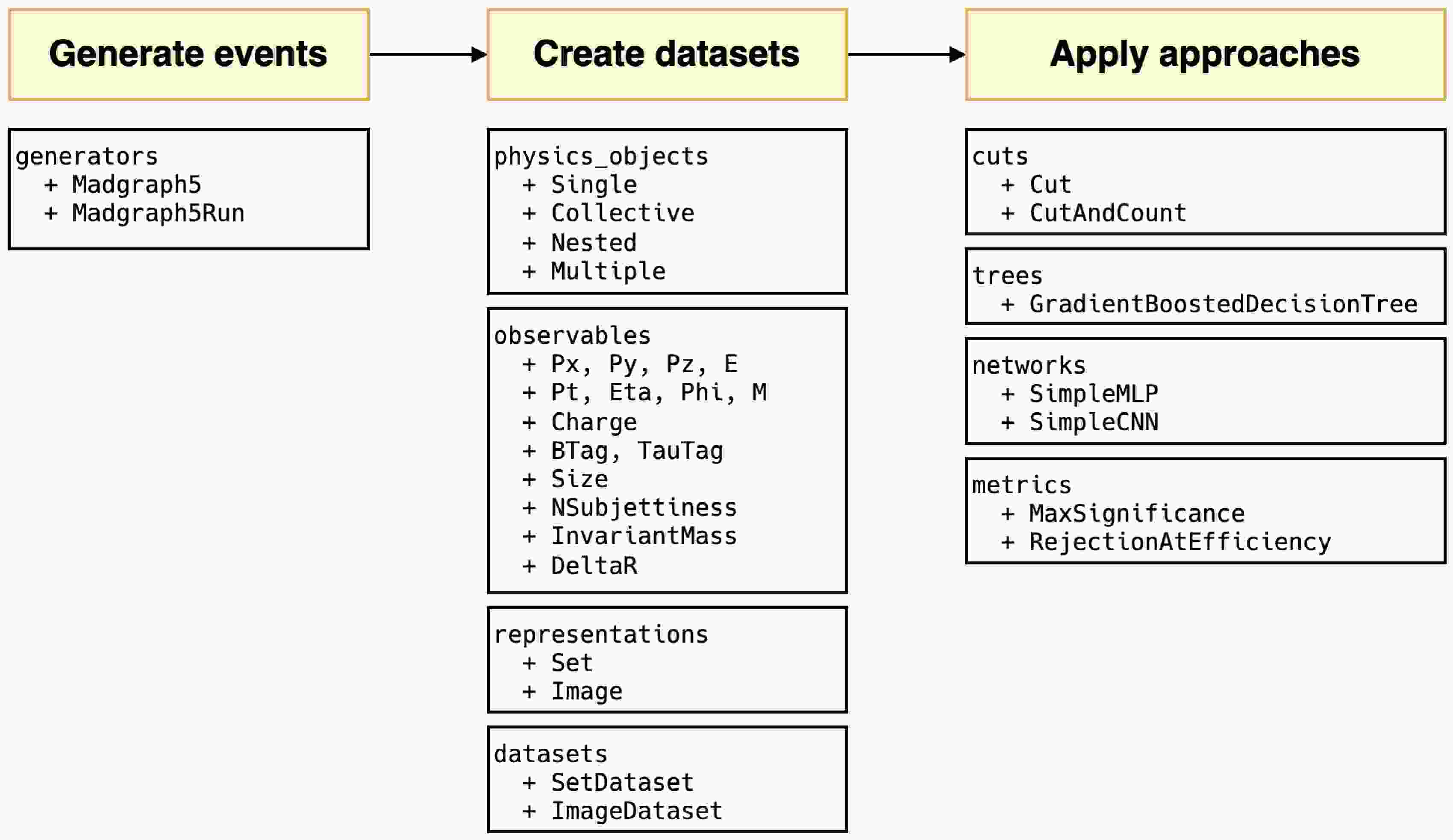
HEP ML LAB, developed in Python, encompasses an end-to-end complete process. All modules are shown briefly in Figure 1. MADGRAPH5_AMC is minimally encapsulated for event generation, such as defining processes, generating Feynman diagrams, and launching runs. In the transition from events to datasets, we introduced an observable naming convention that directly links physical objects with observables, facilitating users to directly use the names of observables to retrieve corresponding values. This convention can further apply to the definitions of cuts. Inspired by the expression form of cuts in UPROOT [52], we expand the corresponding syntax to support filtering at the event level, using veto to define events that need to be removed and more complex custom observables. When creating datasets with different representations, this naming rule still applies. In the current version, users can easily create set and image datasets, and for images, we also offer a rich set of functions for preprocessing and displaying.

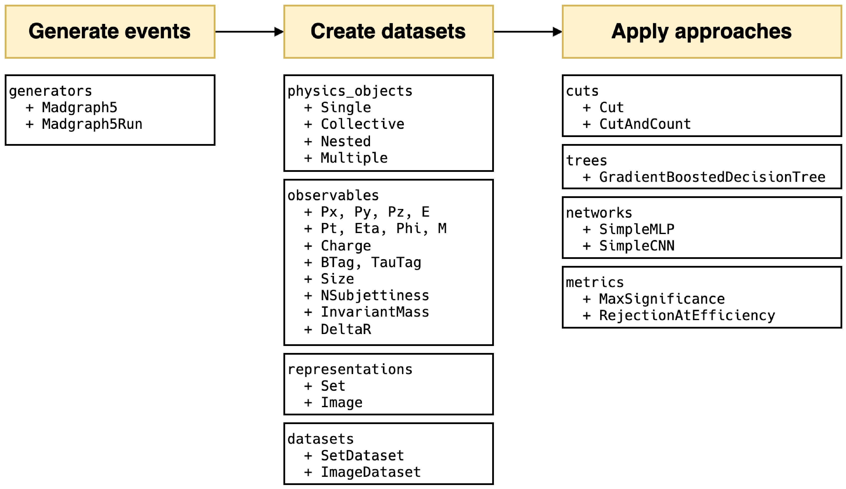
Figure 1.  (color online) All modules in the $ \mathrm{hml}$ framework and main classes in each module.

In the part of machine learning, we introduce two basic deep learning models: simple multi-layer perceptron and simple convolutional neural network. Both have fewer than ten thousand parameters, providing a baseline for classification performance. These models are implemented using KERAS [53] without any custom modifications, making it easy to expand to other existing models. Additionally, we integrate two traditional approaches, cut-and-count, and gradient boosted decision tree, ensuring compatibility with KERAS. After different approaches are trained, we provide physics-based evaluation metrics: signal significance and background rejection rate at fixed signal efficiency, to assess their performance.

This package is publicly available through the Python Package Index (PyPI) and can be installed using the standard pip package manager with the command $ \mathrm{pip install hep-ml-lab}$. It supports Python 3.9+ and is compatible with Linux, MacOS, and Windows operating systems. The source code is open-sourced at Github ¹.

The structure of the paper is as follows. The section 2 introduces the wrapper class of MADGRAPH5_AMC to generate events. In the section 3, we describe the observable naming convention and show step by step how it is used to extract data from events and extended to filter data and to create datasets. Three types of approaches: cut and count, decision trees, and neural networks available now are shown in the section 4. Physics-inspired metrics are also included there. In the section 5, we demonstrate the effectiveness of the framework by a simple and complete W boson tagging as a case study. Finally, we conclude the paper and discuss the future work in the section 6.

All phenomenological studies generally start from simulating collision events, for example using MADGRAPH5_AMC. The $ \mathrm{generators}$ module provides a wrapper for parts of its core functionalities, aiming to facilitate its integration into Python scripts for customized setting requirements.

Code example 1: Initialize $ \mathrm{Madgraph5}$.

In code example 1, users need to pass the executable path to the $ \mathrm{executive}$ parameter to ensure commands can be sent to it. The $ \mathrm{verbose}$ parameter controls whether to display intermediate outputs, with the default value of 1, meaning they are displayed, consistent with the output seen when using MADGRAPH5_AMC in the terminal. After initialization, we can use its various methods to simulate commands entered in the terminal as shown in code example 2.

Code example 2: Methods of $ \mathrm{Madgraph5}$ to generate processes.

During the process generation, we first need to use the $ {\mathrm{import}}{\_}{\mathrm{model}}$ method to import the model file. This method supports passing the path of the model or the name of the model (MADGRAPH5_AMC will search for the model in the models folder or download the model based on its name). Next, use the $ \mathrm{define}$ method to define multi-particles, for example, ${\mathrm{define ("j = }} $ $ { \mathrm{j b b}}\sim {\mathrm "})$. Then, in the $ \mathrm{generate}$ method, pass in all the processes to be generated without having to input $ \mathrm{add process}$ like in the terminal. Here, the asterisk represents the unpacking operation in Python, and you can directly enter multiple processes separated by commas $ \mathrm{g.generate("p p > w+ z", "p p > } \mathrm{w- z")}$ without needing to construct a list with square brackets. Usually, to confirm processes have been generated as expected, we need to view the Feynman diagrams, at which point the ${ \mathrm{display}}\_{ \mathrm{diagrams}}$ method can be used. It saves the generated Feynman diagrams to the ${ \mathrm{diagram}}\_{ \mathrm{dir}}$ folder and has already converted the default eps files into pdf format for convenience. Finally, use the $ \mathrm{output}$ method to export the processes to a folder.

Code example 3: Use $ \mathrm{launch}$ method and set up all possible parameters for generating events.

With the process folder ready, we can start to produce runs to generate simulated events as shown in code example 3. The $ \mathrm{launch}$ method includes parameters you may need to configure for the run, where $ \mathrm{shower}$, $ \mathrm{detector}$, $ \mathrm{madspin}$ represent switches for PYTHIA8, DELPHES, and MADSPIN, respectively, consistent with the options in the terminal's prompt.$ \mathrm{settings}$ includes parameters configured in the run card, for example, $ \mathrm{settings = \{"nevents": 1000, "iseed": 42\}}$. While $ \mathrm{iseed}$ is the random seed used by MADGRAPH5_AMC to control the randomness of the sub-level events, it does not affect PYTHIA8 and DELPHES. You can specify the $ \mathrm{seed}$ parameter to uniformly configure these three, ensuring the cross section, error, and events are fully reproducible. The $ \mathrm{decays}$ method is used to set the decay of particles, for example, $ \mathrm{decays = ["w+ > j j", "z > vl vl}\sim{\mathrm{"}}]$. The $ \mathrm{cards}$ parameter accepts the path to your pre-configured parameter files, for example, ${ \mathrm{cards = ["delphes}}\_{ \mathrm{card.dat"}}, $ $ { \mathrm{"pythia8}}\_{ \mathrm{card.dat"]}}$. In this version, only Pythia8 and Delphes cards can be recognized correctly with "pythia8" and "delphes" in their file names. It currently doesn't support the cards that have external folders as dependencies like the muon collider delphes card. When a large number of events need to be generated, you can set the $ {\mathrm{multi}}\_{ \mathrm{run}}$ parameter to create multiple sub-runs for a single run, for example, setting $ {\mathrm{multi}}\_{\mathrm{run}} = 2$, the final event files will be named in the form of $ {\mathrm{run}}\_01\_1$, $ {\mathrm{run}}\_01\_2$, which is controled by $ \mathrm{MadEvent}$. Note, since MADGRAPH5_AMC does not recommend generating more than one million events in a single run, the $ \mathrm{nevents}$ parameter in $ \mathrm{settings}$ should also be set appropriately, as the total number of events is the result of $ \mathrm{nevents}$ multiplied by $ {\mathrm{multi}}\_{\mathrm{run}}$. $ \mathrm{hml}$ will generate the corresponding valid commands based on your settings and send them to MADGRAPH5_AMC running in the background. If you want to check the actual commands before the run starts, you can set $ {\mathrm{dry}} ={\mathrm{ True}}$, which returns the generated commands instead of starting the run.

Code example 4: All the information seen in the table can be accessed.

After generating the events, you can use the $ \mathrm{summary}$ method, i.e., $ \mathrm{g.summary()}$ to print the results in a table as shown in Figure 2. The table includes the name of each run, the number of sub-runs in brackets, colliding particle beam information, tags, cross-section, error, total number of events, and the random seed. The header displays process information, and the footnote shows the output's relative path, essentially consistent with the results you see on the web page.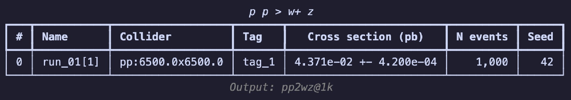

Figure 2.  (color online) The output of $ \mathrm{summary}$ method.

If you wish to continue experimenting with different parameter combinations, you can use the $ \mathrm{launch}$ method again, or employ Python's loop statements to generate a series of combinations to observe the differences in cross-section under various conditions. When doing so, it is recommended to set short label names to facilitate subsequent search and analysis like code example 5 does.

Code example 5: Use a loop to scan the mass of a particle called "nh2" and show the summary.

If there're already output files and you can use $ \mathrm{hml}$ to extract some information for subsequent use. The class method ${ \mathrm{Madgraph5.from}}\_{\mathrm{output}}$ and the $ \mathrm{Madgraph5Run}$ will be of great assistance as shown in 6. The former accepts the path to the output folder, which is the path you enter in the $ \mathrm{output}$ command of $ \mathrm{MadGraph5}$, as well as the path to the executable file. The latter requires the output folder path and the name of the run to access information such as cross section and error. The $ \mathrm{events}$ method allows for retrieving the paths to all event files under a run, including sub-runs. Currently, it only supports files in root format. You can use $ \mathrm{uproot}$ to open these files for subsequent processing.

Code example 6: Use $ {\mathrm{Madgraph5.from}}\_{\mathrm{output}}$ and $ \mathrm{Madgraph5Run}$ to access the information.

The leading fat jet's mass, the angular distance between the primary and secondary jets, the total transverse momentum of all jets, the number of electrons, etc., all demonstrate that observables are always connected to certain physical objects. Thus, we propose the observable naming convention: the name of an observable is a combination of the physical object's name and the type of observable, connected by a dot, denoted as $ \mathrm{<physics object>.<observable type>}$. In this section, starting from physical objects, we gradually refine this representation, eventually extending it to the acquisition of observables, the construction of data representations, and the definitions of cuts.

Physical objects in DELPHES are stored in different branches, representing a category rather than a specific instance. Considering that the calculation of many observables involves different types and numbers of physical objects, often utilizing their fundamental four-momentum information, we have categorized physical objects into four types based on their quantity and category:

1. $ \mathrm{Single}$ physical objects, which precisely refer to a specific physical object. For example:

– $ \mathrm{"jet0"}$ is the leading jet.

– $ \mathrm{"electron1"}$ is the secondary electron.

2. $ \mathrm{Collective}$ physical objects, representing a category of physical objects. For example:

– $ \mathrm{"jet"}$ or $ \mathrm{"jet:"}$ represents all jets.

– $ \mathrm{"electron:2"}$ represents the first two electrons.

3. $ \mathrm{Nested}$ physical objects, formed by free combinations of single and collective physical objects. It currently supports the combination of "FatJet/Jet" and "Constituents":

– $ \mathrm{"jet.constituents"}$ represents all constituents of all jets.

– $ \mathrm{"fatjet0.constituents:100"}$ represents the first 100 constituents of the leading fat jet.

4. $ \mathrm{Multiple}$ physical objects, composed of the previous three types and separated by commas. For example:

– $ \mathrm{"jet0,jet1"}$ represents the leading and secondary jets.

This naming convention is inspired by the syntax of Python lists. To minimize the input cost for the user, we discard the original requirement to use square brackets for receiving indexes or slices: for single physical objects, the type name is directly connected to the index value; for collective physical objects, a colon is used to separate the start index from the end index, and the type name alone represents the whole. Use ${ \mathrm{parse}}\_{\mathrm{physics}}\_{\mathrm{object}}$ method to get the branch and the required index values based on the name of the physical objects as shown in code example 7. This design makes users focus on the physical objects themselves, rather than on how the corresponding classes should be initialized. In Table 1, we also summarize all types of physical objects, their initialization parameters, and examples.

Type	Initialization parameters	Name examples
$\mathrm{Single}$	$\mathrm{branch: str,}$ $\mathrm{index: int}$	$\mathrm{"jet0", "muon0"}$
$\mathrm{Collective}$	$\mathrm{branch: str,}$ $\mathrm{start: int|None}$	$\mathrm{"jet", "jet1:", "jet:3", "jet1:3}$
$\mathrm{Nested}$	$\mathrm{main: str|PhysicsObject,}$ $\mathrm{sub: str|PhysicsObject}$	$\mathrm{"jet.constituents", "jet0.constituents:100}$
$\mathrm{Multiple}$	$\mathrm{all: list[str|Physicsobject]}$	$\mathrm{"jet0,jet1", "jet0,jet"}$

Table 1.  All types of physics objects and their examples.

Code example 7: Use $ {\mathrm{parse}}\_{\mathrm{physics}}\_{\mathrm{object}}$ method to get the branch and slices of physics objects.

In this version, physical objects are merely tools for parsing user input and do not contain any information about observables. Unlike other software packages, we strictly separate the acquisition of observables from the physical objects. Physical objects only store information about the connection between observables and their data sources, not the data itself.

After defining physical objects, the task of observables is to extract information from them. In code example 7, we store all useful information from a physical object in $ \mathrm{branch}$ and $ \mathrm{slices}$: the former refers to the corresponding branch name, and the latter means a specific parts of array-like data. The advantage of doing so is that when encountering certain physical objects, such as the hundredth jet, which does not exist, it returns a list of length zero instead of an error. An empty list will automatically be judged as $ \mathrm{False}$ when applying cuts, thereby being skipped.

In Table 2, we list all the observables currently available. To avoid remembering exact name of an observable, its name is case-insensitive and common aliases are added. For example, $ \mathrm{Mass}$ can be written as $ \mathrm{mass}$ or $ \mathrm{m}$, and $ \mathrm{NSubjettinessRatio}$ has the alias $ \mathrm{tau{m}{n}}$, where the values of $ \mathrm{m}$ and $ \mathrm{n}$ are passed as parameters into the corresponding class. For the transverse momentum, considering the style in different softwares, we more aliases for its symbol representation. Moreover, different observables support different types of physical objects. For example, the $ \mathrm{Size}$ observable supports collective physical objects, while the $ \mathrm{AngularDistance}$ observable supports all combinations of multi-body objects.

Type	Alias	Single	Collective	Nested	Multiple
$\mathrm{MomentumX, Px}$	${\mathrm{momentum}}\_{\mathrm{x, px}}$	$\checkmark$	$\checkmark$	$\checkmark$
$\mathrm{MomentumY, Py}$	${\mathrm{momentum}}\_{\mathrm{y, py}}$	$\checkmark$	$\checkmark$	$\checkmark$
$\mathrm{MomentumZ, Pz}$	${\mathrm{momentum}}\_{\mathrm{z, pz}}$	$\checkmark$	$\checkmark$	$\checkmark$
$\mathrm{Energy, E}$	$\mathrm{energy, e}$	$\checkmark$	$\checkmark$	$\checkmark$
$\mathrm{TransverseMomentum, Pt}$	${\mathrm{transverse}}\_{\mathrm{momentum, pt, pT, PT}}$	$\checkmark$	$\checkmark$	$\checkmark$
$\mathrm{PseudoRapidity, Eta}$	${\mathrm{pseudo}}\_{\mathrm{rapadity, eta}}$	$\checkmark$	$\checkmark$	$\checkmark$
$\mathrm{AzimuthalAngle, Phi}$	${\mathrm{azimuthal}}\_{\mathrm{angle, phi}}$	$\checkmark$	$\checkmark$	$\checkmark$
$\mathrm{Mass, M}$	$\mathrm{mass, m}$	$\checkmark$	$\checkmark$	$\checkmark$
$\mathrm{Charge}$	$\mathrm{charge}$	$\checkmark$	$\checkmark$
$\mathrm{BTag}$	${\mathrm{b}}\_{\mathrm{tag}}$	$\checkmark$	$\checkmark$
$\mathrm{TauTag}$	${\mathrm{tau}}\_{\mathrm{tag}}$	$\checkmark$	$\checkmark$
$\mathrm{NSubjettiness, TauN}$	${\mathrm{n}}\_{\mathrm{subjettiness,tau}}\_{\mathrm{n},}{\mathrm{ tau{n}}}$	$\checkmark$	$\checkmark$
$\mathrm{NSubjettinessRatio, TauMN}$	${\mathrm{n}}\_{\mathrm{subjettiness}}\_{\mathrm{ratio, tau}}\_{\mathrm{{m}{n}, tau{m}{n}}}$	$\checkmark$	$\checkmark$
$\mathrm{Size}$	$\mathrm{size}$		$\checkmark$
$\mathrm{InvariantMass}$	${\mathrm{invariant}}\_{\mathrm{mass, inv}}\_{\mathrm{mass, inv}}\_{\mathrm{m}}$	$\checkmark$			$\checkmark$
$\mathrm{AngularDistance, DeltaR}$	${\mathrm{angular}}\_{\mathrm{distance, delta}}\_{\mathrm r}$	$\checkmark$	$\checkmark$	$\checkmark$	$\checkmark$

Table 2.  All types of observables and their supported types of physical objects.

In code example 8, we show how to use such an observable. First initialize the corresponding observables using the $ {\mathrm{parse}}\_{\mathrm{observable}}$ function from the $ \mathrm{observables}$ module, then use the $ \mathrm{read}$ method to extract the values from an event. As the $ \mathrm{read}$ returns the object itself, you can take the advantage of method chaining to define an observable directly followed by reading an event. We also add extra information when you print the observable itself: its name, shape, and data type. Internally, $ \mathrm{awkward}$[54] is used for manipulating variable-lengthed jagged arrays. The question mark in the data type indicates there are missing values ($ \mathrm{None}$). The $ \mathrm{var}$ appearing in the shape indicates inconsistent lengths, for example, each event has a varying number of jets and each jet has a varying number of constituents.

While the first dimension of the observable value always represents the number of events, the shape is generally determined by the related physical objects. For example, the shape of transverse momentum and other kinematic variables is exactly as its physics obsject. However, this also depends on how to compute the observable. For instance, the shape of the $ \mathrm{Size}$ observable is the number of physics objects and the second dimension is always $ 1 $, whereas the shape of $ \mathrm{AngularDistance}$ depends on the type of physical objects: if calculating the distance between all jets and the leading fat jet, we will get an array of shape ${ \mathrm{(n}}\_{\mathrm{events, var, 1)}}$, where ${ \mathrm{n}}\_{\mathrm{events}}$ represents the number of events, $ \mathrm{var}$ represents a variable number of jets, and $ 1 $ represents the leading fat jet; if calculating the distance between the first ten fat jets and all constituents of all jets, we obtain an array of shape $ {\mathrm{(n}}\_{\mathrm{events, 10, var)}}$. The $ \mathrm{var}$ now comes from the number of constituents and the number of jets, which we compress two dimensions into one. For events that do not have enough physics objects, the missing values are filled with $ \mathrm{None}$.

Code example 8: Use $ {\mathrm{parse}}\_{\mathrm{observable}}$ and $ \mathrm{read}$ to get the value of observables. $ \mathrm{events}$ are opened by $ \mathrm{uproot}$.

The built-in observables are only some of the most basic ones, so they may not be sufficient for every use case. Therefore, we show three examples of building your own observables. In the first example 9, when the needed observable is already stored under a certain branch, you only need to declare the name of this observable as a class that inherits from $ \mathrm{Observable}$. $ \mathrm{hml}$ will search for the branch based on the physical object name and extract the corresponding value based on the slices. Here, we take the observable $ \mathrm{MET}$ as an example, which is originally stored under the branch $ \mathrm{MissingET}$. To use the $ {\mathrm{parse}}\_{\mathrm{observable}}$ function, you can call ${\mathrm{register}}\_ $ $ {\mathrm{observable}}$ function to register an alias for it. Please note that this implementation requires a physical object, which means that only by entering $ \mathrm{"missinget0.met"}$ or $ \mathrm{"MissingET0.MET"}$ can the ${ \mathrm{parse}}\_{\mathrm{observables}}$ works as normal. Only $ \mathrm{"MET"}$ or $ \mathrm{"met"}$ without an physics object is not allowed. As each event has only one missing energy physical object, $ \mathrm{"MissingET"}$ is followed by 0.

Code example 9: Inherit from $ \mathrm{Observable}$ and it will automatically retrieve the corresponding value if the physics object does have it.

If you already have established a computation process and do not want to consider the physical objects, we recommend referring to the second example 10. All you need to do is overwrite the $ \mathrm{read}$ method, defining how to compute the values of observables. The $ \mathrm{events}$ is the return value of $ \mathrm{uproot.open}$. You may need to adjust the calculation due to the $ \mathrm{events}$ and the underlying $ \mathrm{awkward}$ array. It is important to note that $ \_\mathrm{value}$ must be an iterable object, such as a list or array, to be correctly converted into an $ \mathrm{awkward}$ array by $ \mathrm{hml}$. Additionally, you should return $ \mathrm{self}$ at the end, enabling chain calls similar to other observables.

Code example 10: Overwrite the $ \mathrm{read}$ method to define how to calculate the value of the observable.

The third example 11 changes the initialization. We add constraints on physical objects, i.e. it could only be related to a single physics object. There's also a new parameter for more flexibility. The $ \mathrm{read}$ part is the same as the second example. This is the strictest observable but also the safest one.

Currently, the naming convention is built upon the output of DELPHES and does not support other formats yet. However, considering that different analyses require data at different levels and in different formats, we plan to gradually add support for other event formats in future versions, such as HEPMC, LHE, etc.

To make high-energy physics data compatible with different analysis approaches, it necessary to convert data into various representations. The review [55] summarizes six representations of jets: ordered sets, images, sequences, binary trees, graphs, and unordered sets. Built upon the observable naming convention, we extend the representation to an event. Currently, $ \mathrm{hml}$ supports the (ordered) set and image representations. In future versions, we will prioritize adding the graph representation and corresponding neural networks.

Code example 11: Define an observable with constraints on the type of physical objects and with a new parameter.

The ordered set is one of the most commonly used representations. It arranges physics-inspired observables in an arbitrary order to form a vector that describes an event. The vectors from all events are then assembled into one matrix by event, with the shape $ {\mathrm{(n}}\_{\mathrm{events, n}}\_{\mathrm{observables)}}$. Following the naming convention, it is straightforward and concise to construct such a set as illustrated in code example 12.

Code example 12: Use $ \mathrm{Set}$ to represent the ordered set of observables.

You need to package the observable names into a list and pass it into the $ \mathrm{Set}$, then call the $ \mathrm{read}$ method to get the values from events. The values will be stored in the $ \mathrm{values}$ attribute. Here, you can see that we use $ \mathrm{awkward}$ arrays to store data. For observables with the correct physical object name but not existing (for example, $ \mathrm{muon0.charge}$, when there are no muons produced in the event), we treat its value as $ \mathrm{None}$. This way of handling missing values allows us to follow the matrix operation habit: first build the data matrix, then deal with the missing values.

For the image representation, we also use observable names to define the way of fetching the data for its height, width, and channel, as shown in code example 13. The $ \mathrm{read}$ method is used to read events as before. Here, we construct an image of the leading fat jet, with all its constituents' pseudorapidity, azimuthal angle, and transverse momentum. Considering the significant amount of works that includes similar preprocessing processes, we add them as the methods of the $ \mathrm{Image}$ class. Since the preprocessing often relates to sub-jets, it's necessary to add information about sub-jets via the method $ {\mathrm{with}}\_{\mathrm{subjets}}$: its parameters include the name of constituents, clustering algorithm, radius, and the jet's minimum momentum. The $ \mathrm{translate}$ method moves the position of the leading sub-jet to the origin, which reduces the complexity of position information helping speed up the learning process. Next, for the sub-leading sub-jet, it can be rotated right below the origin, making the features of the entire image more pronounced. Lastly, the $ \mathrm{pixelate}$ method is used to pixelate the data to make up an real image. Since pixelation leads to a reduction in data precision, this step is separated out, allowing for further studies on when to apply it and the impacts of the order.

Code example 13: Use $ \mathrm{Image}$ to represent a fat jet and preprocess it via sub-jets.

For convenience in displaying images, the $ \mathrm{Image}$ class contains a $ \mathrm{show}$ method that can directly plot it as an image. Code example 14 shows all the available parameters: the first two are used to show the image as dots, and the last three parameters display a pixel-level grid, enable the grid by default, and apply normalization over the whole image, respectively. The Figure 3 shows an image representation before and after preprocessing steps. In the raw image, the observables used for "height" and "width" are directly plotted as a 2D scatter image. For the final pixelated image, $ \mathrm{norm="log"}$ enhances its features more distinctly. The data can be accessed via $ \mathrm{.values}$ property as a list of awkward array (before pixelation) or one awkward array (after pixelation). You can convert them and then save them in formats like numpy array, JSON files to handle them with tools you're more familiar with.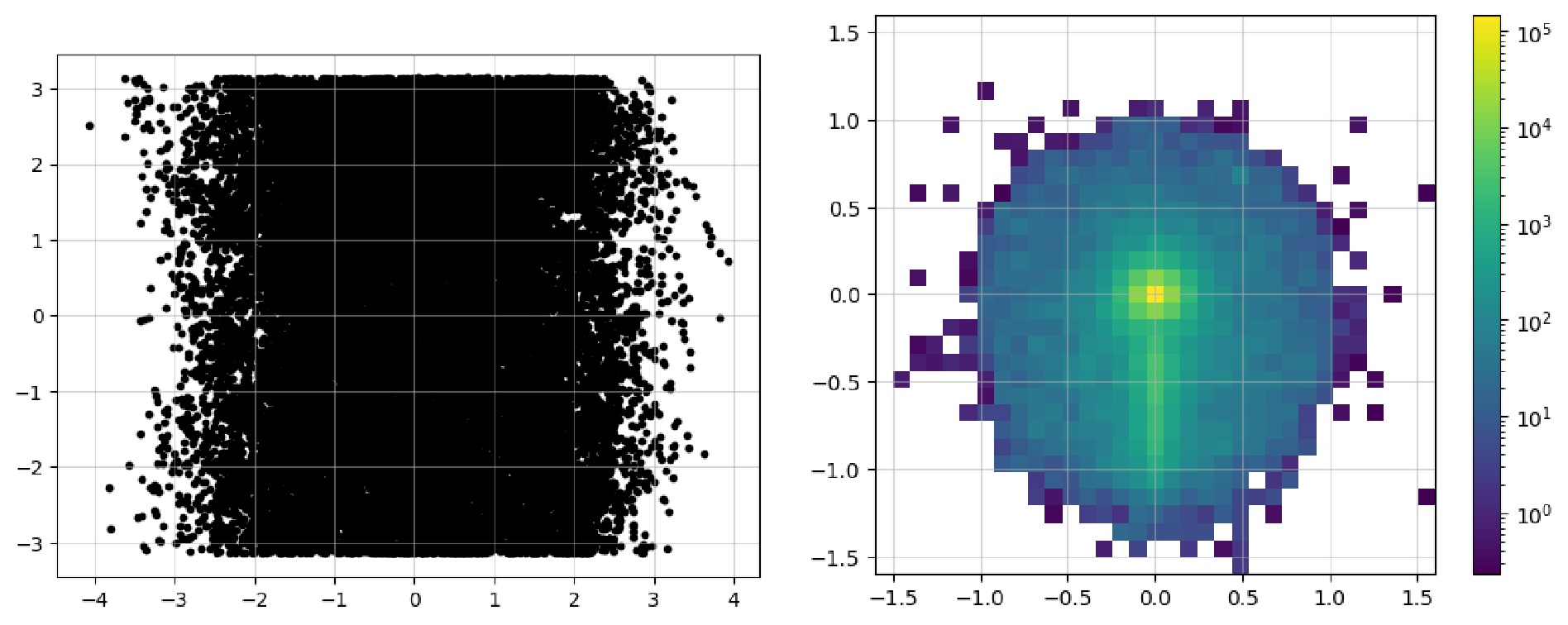

Figure 3.  (color online) The raw image and the pixelated image after preprocessing.

Code example 14: Use $ \mathrm{show}$ to plot the image as a 2d heatmap if it has been pixelated or as a 2d scatter plot.

After acquiring the original event data, it's time to filter it to obtain events that satisfy specific criteria. In the old workflow, during the event loop, it was common to manually include the calculation of observables and then apply conditionals to filter events. We note that the $ ($array) method in $ \mathrm{uproot}$ supports $ \mathrm{cut}$ parameter. In $ \mathrm{hml}$, we utilize a matrix-oriented programming style to change the filtering procedure into boolean indexing; furthermore, we add logical operation syntax upon the observable naming convention to make the definition of cuts intuitive, as shown in code example 15. $ \mathrm{Cut}$ still has the similar $ \mathrm{read}$ method. The values form a one-dimensional boolean matrix, length of which is equal to the number of events. It allows you to directly use it to filter other observables via boolean indexing.

For the extend syntax of logical operations, i.e. how to combine multiple conditions, we referr to the implementation of $ \mathrm{uproot}$: it uses the bitwise logical operators of matrices, & and $ \mathrm{|}$ to replace $ \mathrm{and}$ or $ \mathrm{or}$, and adding parentheses to ensure priority. For example, $ \mathrm{(pt1 > 50) }$ & $ \mathrm{ ((E1>100) | (E1<90))}$ expresses the condition that $ \mathrm{pt1}$ is greater than 50 and $ \mathrm{E1}$ is either greater than 100 or less than 90. The expression is then parsed directly by Python: it is purely matrix operation, without considering the case of DELPHES output. It cannot handle such cuts: "all jets are required to have transverse momentum greater than 10 GeV", whose data is of shape ${ \mathrm{n}}\_{\mathrm{events, var}}$. It undoubtedly requires users to rearrange the original data to make the dimensions of the matrices consistent since the number of jets is not necessarily the same among events. This essentially only filters values that meet the conditions, not the events that meet the conditions. In conjunction with the observable naming convention, we advocate simplifying the matrix logical operation syntax to facilitate user input.

Code example 15: Cut values are boolean arrays that can be used to filter other observables.

1. Logical AND and logical OR are still represented by $ \mathrm{and}$ or $ \mathrm{or}$. They are converted into bitwise logical operators & and $ \mathrm{|}$ automatically, avoiding too many parentheses;

2. The result of the logical expression acts on the first dimension, that is, the dimension of events, to filter events;

3. Involved observables must have the same dimensions to ensure the correctness of logical operations;

4. At the end of a cut, default $ \mathrm{[all]}$ represents a logical AND operation on all values of all observables in each event. It can be ignored and not written; $ \mathrm{[any]}$ represents a logical OR operation on all values of all observables in each event. This syntax is suitable for cases where all of a certain observable or any one observable in the events needs to meet the conditions;

5. Add support for $ \mathrm{veto}$ at the beginning of a cut for cases where certain events need to be excluded.

Below, we take specific literatures to demonstrate and explain the new syntax. The original text will be presented first, followed by the corresponding cut in the next line. We assume that data is stored in the same units as the description indicates. In the literature [56]:

1. Muons $ \mu^{ \pm} $ are identified with a minimum transverse momentum $ p_T^\mu>10 \mathrm{GeV} $ and rapidity range $ \left|\eta^\mu\right|<2.4 $...

$ \mathrm{muon.pt > = 10 and -2.4 < muon.eta < 2.4}$

Here, we take all the muons and simplify the syntax for pseudorapidity within a certain range, which can be written consecutively. Here, the $ \mathrm{and}$ represents the bitwise logical operator of the matrix. For each event, if there is no $ \mathrm{[any]}$ at the end of the expression, it means that all values need to satisfy the condition;

2. Only events with reconstructed di-muons having same sign are selected.

$ \mathrm{muon0.charge = = muon1.charge}$

Here, we only need to judge whether the charges of the two muons are the same, without determining whether the number of muons is two. When there are fewer than two muons, the charge of one muon will be $ \mathrm{None}$, and such judgment will be automatically treated as $ \mathrm{False}$;

3. We identify the hardest fat-jet with the $ W^{ \pm} $ candidate jet ($ J $) and this is required to have $ p_T^J>100 \mathrm{GeV} $.

$ \mathrm{fatjet0.pt > = 100}$

In the literature [57]:

1. C3: we veto events if the OS di-muon invariant mass is less than 200 GeV.

${ \mathrm{muon0.charge ! = muon1.charge and muon0,muon1.inv}}$ $\_{\mathrm{mass > 200}} $

2. C4: we apply a b-veto.

$ {\mathrm{veto jet.b}}\_{\mathrm{tag = = 1 [any]}}$

Use $ \mathrm{veto}$ and $ \mathrm{[any]}$ to indicate that for all jets, if any one of them is b-tagged, then the event is excluded.

3. C5: we consider only events with a maximum MET of 60 GeV.

$ \mathrm{MissingET0.PT < 60}$

Using uppercase and lowercase is equivalent because there is only one missing energy, so it is represented by 0. The MET observable here actually also refers to the transverse momentum, so it can be represented by PT.

4. C8: we choose events with $ N $-subjettiness $ \tau_{21}^{J_0}<0.4 $.

$ \mathrm{fatjet0.tau21 < 0.4}$

The definition of this observable is provided by the DELPHES card. We have already defined its parsing method in the observables module, so here we can directly use its name.

In the literature [58], the cuts of CBA-I for $ M_N = 600-900 $ GeV:

1. Jet-lepton separation $ 2.8<\Delta R(j, \ell)<3.8 $

$ {\mathrm{ 2.8 < jet0,lepton0.delta}}\_{\_{\mathrm{mass > 200}}{r < 3.8}}$

In the literature [59]:

1. The basic selections in our signal region require a lepton ($ e $ or $ \mu $) with $ |\eta_{\ell}|<2.5 $ and $ p_{T, \ell}>500 $ GeV...

$ \mathrm{ -2.5 < muon0.eta < 2.5 and muon0.pt > 500}$.

We take the muon as the example.

2. ... veto events that contain additional leptons with $ \left|\eta_{\ell}\right|<2.5 $ and $ p_{T, \ell}>7 \mathrm{GeV} $

$ \mathrm{veto -2.5 < muon.eta < 2.5 and muon.pt >}$ $ \mathrm{7 [any]} $

In this cut, it's easier to use $ \mathrm{veto}$ to exclude events with additional leptons.

3. ... and impose a jet veto on subleading jets with $ \left|\eta_j\right|<2.5 $ and $ p_{T, j}>30 \mathrm{GeV} $.

$ \mathrm{veto -2.5 < jet1.eta < 2.5 and jet1.pt > }$ $\mathrm {30 [any]}$

In the literature [60]:

1. Photon-veto: Events having any photon with $ p_T>15 $ GeV in the central region, $ |\eta|<2.5 $ are discarded.

$ \mathrm{veto -2.5 < photon.eta < 2.5 and photon.pt }$ $\mathrm{> 15 [any] }$

2. $ \tau $ and b-veto: No tau-tagged jets in $ |\eta|<2.3 $ with $ p_T>18 $ GeV, and no b-tagged jets in $ |\eta|<2.5 $ with $ p_T>20 $ GeV are allowed.

$ {\mathrm{ veto jet.tau}}\_{\mathrm{tag = = 1 and -2.3 < jet.eta < }}$ ${\mathrm{2.3 and jet.pt > 18 [any] }}$

3. Alignment of MET with respect to jet directions: Azimuthal angle separation between the reconstructed jet with the MET to satisfy $ \min (\varDelta \phi({\bf{p}}_T^{\mathrm{MET}}, {\bf{p}}_T^j))>0.5 $ for up to four leading jets with $ p_T>30 \mathrm{GeV} $ and $ |\eta| < 4.7 $.

${\mathrm{jet:4,missinget0.min}}\_{\mathrm{delta}}\_{\mathrm{phi > 0.5 and }}$ ${\mathrm{jet:4.pt >}} {\mathrm{30 and -4.7 < jet:4.eta < 4.7}} $

Users need to define the observable $ \mathrm{MinDeltaPhi}$ in advance and register it with alias $ {\mathrm{min}}\_{\mathrm{delta}}\_{\mathrm{phi}}$.

With the data representation and cuts defined previously, we can now proceed to construct the dataset. Corresponding to data representations, we currently offer two datasets: $ \mathrm{SetDataset}$ and $ \mathrm{ImageDataset}$. Code example 16 shows the use of the dataset of an ordered set. Its initialization requires names of the observables. Then still use the $ \mathrm{read}$ method to read events. For this $ \mathrm{read}$, we added two additional parameters: $ \mathrm{targets}$ is the integer label you assign to the event, which is the target of convergence. Here we assign $ 1 $ to denote events as signals; $ \mathrm{cuts}$ are your filtering criteria. Here we require the number of jets to be more than $ 1 $, and the number of leading fat jets to be more than $ 0 $. When you use multiple cuts, the result of each cut is applied to the dataset one by one, which means they are connected by logical AND. When splitting the dataset, you can use the $ \mathrm{split}$ method. Its parameters are the ratios for train, test, and validation sets, here we used 70% of the data as the training set, 20% as the test set, and 10% as the validation set. Before saving the dataset, you can access the $ \mathrm{samples}$ and $ \mathrm{targets}$ to view the stored data, which have already been converted into $ \mathrm{numpy}$ arrays. Finally, use the $ \mathrm{save}$ method to save the dataset to a zip compressed file with $ \mathrm{.ds}$ suffix. Such a file can be loaded by the ${ \mathrm{load}}\_{\mathrm{dataset}}$ function or $ \mathrm{SetDataset.load}$ class method.

Code example 16: Use $ \mathrm{SetDataset}$ to build a dataset representing each event as a set of observables.

To quickly view the distributions of the entire dataset, you can use the $ \mathrm{show}$ method. The code example 17 shows all the available parameters: ${ \mathrm{n}}\_{\mathrm{feature}}\_{\mathrm{per}}\_{\mathrm{line}}$ is the number of observables to display per line, $ {\mathrm{n}}\_{\mathrm{samples}}$ is the number of events to display, and $ \mathrm{target}$ is the label of the events to display.

Code example 17: Use $ \mathrm{show}$ to display the observable distributions of a set dataset.

The construction process of an image dataset is similar to that of an ordered set, as shown in code example 18. When initializing an $ \mathrm{Image}$, you can directly configure the necessary preprocessing steps in method chaining. When the dataset reads events afterwards, these steps will be carried out in sequence.

Code example 18: Use $ \mathrm{ImageDataset}$ to build a dataset representing each event as an image

Code example 19: Use $ \mathrm{show}$ to plot the image of the dataset.

The $ \mathrm{show}$ method of an image dataset enable you to display events as an image as shown in Example 19. By default, the entire dataset's images are compressed into one image. If the original dimensions are $ {\mathrm{n}}\_{\mathrm{events, height, width, channel}}$, the compressed dimensions will be $ \mathrm{height, width, channel}$. While most parameters are the same as those in the $ \mathrm{show}$ method of $ \mathrm{Image}$, two additional parameters are added: $ {\mathrm{n}}\_{\mathrm{samples}}$ is the number of events to display, and $ \mathrm{target}$ is the label of the events to display.

With well-prepared datasets, we can apply different approaches to identify rare new physics signals. The $ \mathrm{approaches}$ module includes cut-and-count, trees, and neural networks. We will gradually add more in the coming versions. The basic design principle of this module is minimal encapsulation to interface with current frameworks, such as SCIKIT-LEARN [61], TENSORFLOW, and PYTORCH. Considering the simplicity, we adopt the Keras-style interface design: decide approach structure at initialization, $ \mathrm{compile}$ for configuring the training process, $ \mathrm{fit}$ for training the approach, and $ \mathrm{predict}$ for prediction on new data. KERAS is originally a high-level encapsulation of TENSORFLOW, but after the version 3, it begins to support multiple backends, offering unprecedented flexibility, which is one of the reasons we choose it. You should note that we only test the compatibility with TensorFlow backend currently.

Cut-and-count (or cut-based analysis) is fundamental and widely used when studying the impact of various observables on the final sensitivity. It provides evidence to support the discovery of new particles and the verification of new theories.

As the name suggests, it involves two steps: applying a series of cuts to distinguish the signal from the background as much as possible, then counting the number of events that pass the cuts. The subsequent distribution, such as invariant mass, is used to determine the nature of the particles involved. These cuts can be applied onto properties of specific particles, such as kinematic quantities, charge, other observables, or other characteristics associated with simulated collision events, like particle states in decay chains. Filtering the data allows focusing on areas of interest, increasing the possibility of discovering new physics.

Applying cuts involves some technique to make the final signal more evident. Typically, one would plot the distribution of observables that reflect signal characteristics and choose the area with a higher signal ratio as the cut range based on manual judgment. There are two issues here: 1) manual judgment is subjective and cannot guarantee the effect of the cut; 2) the observable distributions that people observe is sometimes the source data without any cuts. If there is an unavoidable association between observables, applying a cut will affect the distribution of the next observable. Therefore, a more rigorous way is to apply one cut first, plot the distribution of the next observable, then determine the next cut, and so on.

Code example 20: Initialize the CutAndCount approach

Users can use $ \mathrm{CutAndCount}$ to implement these two different strategies of applying cuts. In code example 20, we demonstrate how to initialize a $ \mathrm{CutAndCount}$ method. You need to specify the number of involved observables, and then an internal $ \mathrm{CutLayer}$ will be created to automatically search for optimal cut values. For each observable, four possible conditions are considered: the signal on the left side, right side, middle, and both sides of the cut. Then, it calculates the user-specified loss function for each case, choosing the one with minimum loss as the final cut. $ {\mathrm{n}}\_{\mathrm{bins}}$ sets the granularity of the data when searching, i.e., the number of bins for the distribution of each observable. A higher number of bins can make the cut more precise but also increases the cost of calculation, which also relates to the size of data and the complexity of its distribution. The principle here is that as long as the data distributions become stable, then the number of bins can be appropriately reduced without affecting the final result. $ \mathrm{topology}$ sets the order or the strategy that cuts are applied: $ \mathrm{parallel}$ means all cuts are independent, and the distributions referred to come from the original data, while $ \mathrm{sequential}$ considers the correlation among cuts, with each cut applied on the basis of the previous one.

In code example 21, we show how to configure and train a $ \mathrm{CutAndCount}$ approach. In the $ \mathrm{compile}$ method, you can specify the optimizer, loss function, and evaluation metrics. For $ \mathrm{CutAndCount}$, the optimizer is unnecessary because it does not use gradient descent methods internally, but rather finds the optimal cut values through a search process. The loss function is used to evaluate the effectiveness of each cut, while the evaluation metrics here will be used to show the performance scores during the training, it is better to evaluate the performance after training all at once. The $ {\mathrm{run}}\_{\mathrm{eagerly = True}}$ is necessary. By default, KERAS uses a computational graph for calculations, which is very efficient for training neural networks. However, $ \mathrm{CutAndCount}$ includes some custom calculations that are not yet fully compatible within the computational graph, so it needs to be set to $ \mathrm{True}$. In the $ \mathrm{fit}$ method, you need to input the samples and targets of the training set, where the batch size should be the minimum number that can reflect the distribution pattern of the data. If your dataset is relatively small and can fit entirely into the GPU's memory, you can set the batch size to the size of the entire training set. Besides, the $ \mathrm{epochs}$ parameter is unnecessary, and the $ \mathrm{callbacks}$ parameter has not been implemented yet, but will be gradually added in future versions.

Decision trees are a common method of classification, and there are many mature frameworks available, such as TMVA [62], XGBOOST [63], SCIKIT-LEARN, etc. TENSORFLOW DECISION FORESTS [64] is also a good choice as it also adopts the KERAS training style. Considering our preference for the multi-backend support, we modify parts of the $ \mathrm{GradientBoostingClassifier}$ code from SCIKIT-LEARN to conform to the same style.

Firstly, the original $ \mathrm{fit}$ method is enhanced to handle input targets in one-hot encoded format. Secondly, support for $ \mathrm{Keras}$ metrics during the training process, such as the commonly used $ \mathrm{"accuracy"}$. Thirdly, the output of its $ \mathrm{predict}$ method is changed to predict probabilities, aligning it with $ \mathrm{Keras}$. Despite these changes, many parameters are still not supported yet: many of the original initialization parameters are related to early stopping, learning rate adjustments, etc., which in $ \mathrm{Keras}$ are implemented through callback functions. Moreover, loss functions are not uniformly customizable in $ \mathrm{scikit-learn}$, so we do not support changing it in $ \mathrm{compile}$ method. In code example 22, we demonstrate the basic usage.

Code example 21: Configure and train the $ \mathrm{CutAndCount}$ approach

Code example 22: Basic usage of the modified $ \mathrm{GradientBoostedDecisionTree}$ approach.

A starting point of $ \mathrm{hml}$ is to provide researchers with existing deep learning models so that they can conduct benchmark tests on their datasets and select the optimal model. At this early development stage, we only offer two basic models: $ \mathrm{SimpleMLP}$ (multi-layer perceptron) and $ \mathrm{SimpleCNN}$ (convolutional neural network). In future versions, after thorough testing, we will gradually add more existing models to provide the utmost convenience.

In KERAS, there are three ways to build a model: 1. Using $ \mathrm{Sequential}$ to stack layers, 2. Using the Functional API to construct more complex topologies, 3. Inheriting from $ \mathrm{Model}$ to declare a subclass for greater flexibility. Considering that the construction of many models is quite complex and requires exposing a certain number of hyper-parameters for tuning, we choose the third way to build the provided models. The Figure 4 shows the structures of two models. The $ \mathrm{SimpleMLP}$ has $ 4386 $ parameters with the inputs are three observables. The $ \mathrm{SimpleCNN}$ has $ 5960 $ parameters with the inputs are images of shape $ (33, 33, 1) $. Both models are shallow and simple, so they do not consume too much computing resource during the training and testing stages.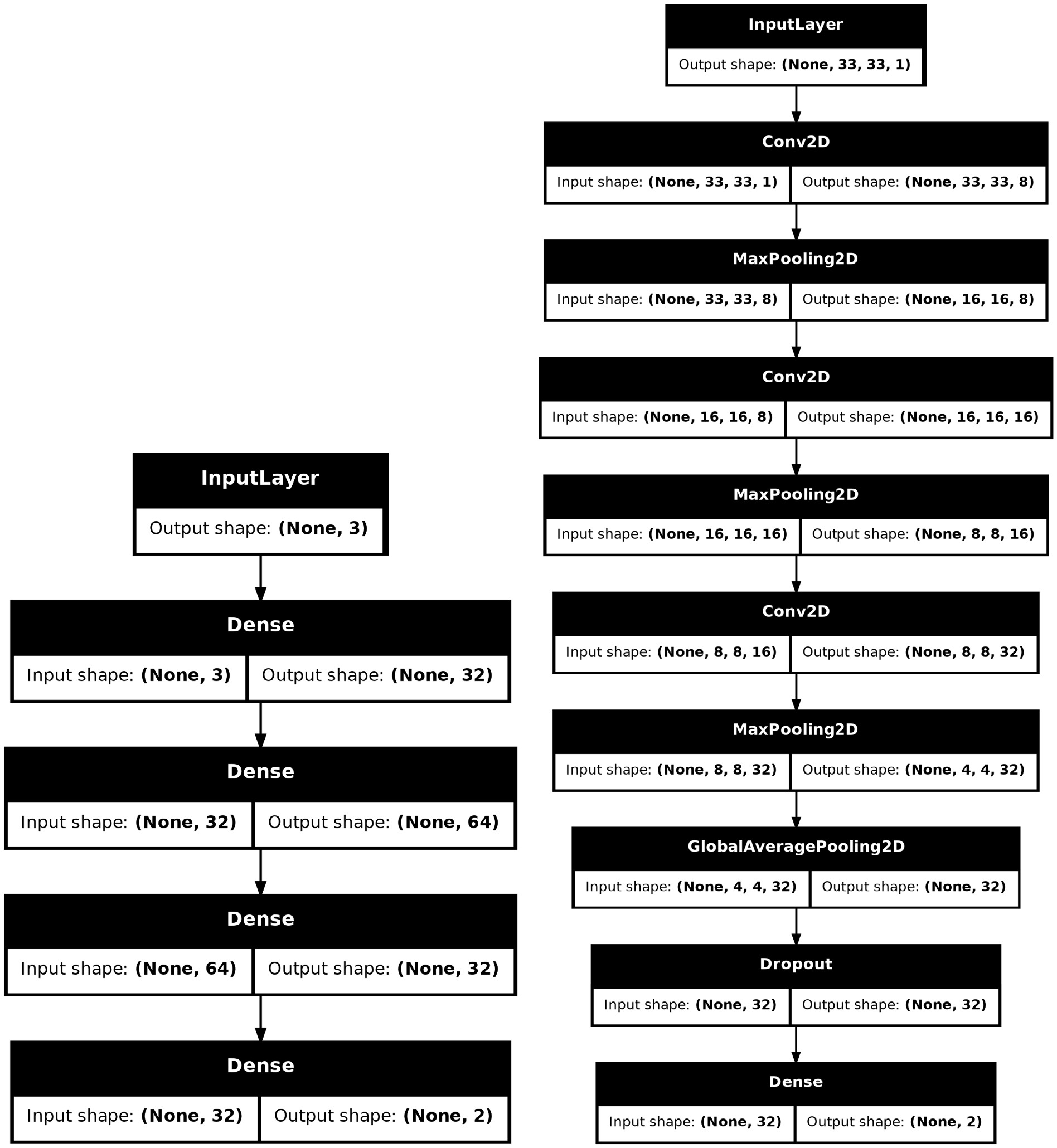

Figure 4.  The structure of the $ \mathrm{SimpleMLP}$ and $ \mathrm{SimpleCNN}$ models.

After training an approach on a dataset, it is often necessary to use various metrics to assess its effectiveness. Unlike the classical accuracy score, which is commonly used in classification tasks, in high-energy physics, the scarcity of signals shifts the focus towards the signal significance, denoted by $ \sigma $. A higher value indicates a lower probability that the observed signal is a result of background fluctuations alone. For instance, 3$ \sigma $ is often considered as an evidence of a signal, indicating that there is about a 0.27% chance of the signal being a statistical fluke. Meanwhile, 5$ \sigma $ is the gold standard in high-energy physics for claiming a discovery, corresponding to a probability of roughly 1 in 3.5 million that the observed signal is due to background noise. Equation 1 is the formula for calculating significance in $ \mathrm{hml}$. Note that here $ S $ represents the number of signals, and $ B $ represents the number of backgrounds, which refer to the number of simulated events when the cross section of the corresponding process and integrated luminosity are not specified. In code example 23 we show how to use it.

Code example 23: Use the $ \mathrm{MaxSignificance}$ metric to evaluate performance of an trained approach.

For the built-in approaches, their outputs are probabilities for signal and background. By default, only when the probability exceeds 0.5 do we consider it as a signal or background. In $ \mathrm{MaxSignificance}$, we can change this threshold by setting $ \mathrm{thresholds}$. By default, data with ${\mathrm{class}}\_{\mathrm{id = 1}}$ is viewed as signal and 0 as background. Change it if the targets for signal and background in your dataset are not like this.

In addition to significance, some literatures also include the background rejection at a fixed signal efficiency as an evaluation metric, so we also support it, shown in equation 2. The higher the background rejection rate, the fewer the number of background events that are mistakenly classified as signals. In the example 24, you can see the same way to use it. Note that for both the metrics, if you call them multiple times, the values will be averaged. So if you want to calculate them from scratch, you need to call the $ {\mathrm{reset}}\_{\mathrm{state}}$ method.

To give users a complete understanding of the entire workflow, this section show how to integrate various modules to complete a task of jet tagging. This example serves merely as a proof of concept; users still need to conduct more personalized analysis on this basis.

We choose to simulate the production of highly boosted $ W^{+} $ bosons that decay into two jets, resulting in a single fat jet during event reconstruction. This jet has distinct characteristics of mass and spatial distributions, making it easier to identify using all built-in approaches.

Code example 24: Use the $ \mathrm{RejectionAtEfficiency}$ metric to evaluate the model's performance.

In code example 25, we first import the event generator module from $ \mathrm{Madgraph5}$ using the $ \mathrm{generate}$ method to create the signal process, and then use the $ \mathrm{output}$ method to save it to a designated folder. To make $ W^{+} $ bosons highly boosted, we leave the decay chain unfinished here and constrain its $ p_T $ range in code example 26. If you want to view the output Feynman diagrams, after the $ \mathrm{output}$ command is completed, you can check them in the $ \mathrm{Diagrams}$ folder inside the output folder.

Code example 25: Generate $ W^{+}$ boson events using $ \mathrm{Madgraph5}$

Then, use the $ \mathrm{launch}$ method in code example 26 to start the simulation, turn on the $ \mathrm{shower}$ and $ \mathrm{detector}$. To boost $ W^+$ boson, we set spin mode as "none" to apply following cuts ² in settings. Following [3], set the $ p_T $ range for the $ W^{+} $ boson from $ 250 $ to $ 350 $ GeV. When using the default CMS delphes card with $ R = 0.8 $ and the anti-$ k_T $ algorithm to cluster the jets, you can obtain a fat jet that is expected to come from the decay of the $ W^{+} $ boson. Use the $ \mathrm{decay}$ method for further specific decays. Set the random seed ($ \mathrm{seed}$) to 42 to ensure the reproducibility of the results. When the simulation ends, use the $ \mathrm{summary}$ method to review the results (shown in Figure 5), akin to viewing results on the website of $ \mathrm{Madgraph5}$.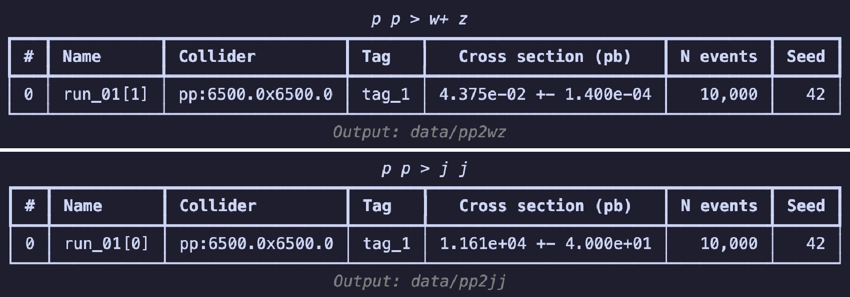

Figure 5.  The summary table of the signal (upper) and background (lower) events.

The generation process for background events is similar 27, with the difference lying in the $ p_T $ range settings. Since the jets in this case do not originate from the decay of a single particle, we directly restrict the $ p_T $ range of the jets.

Code example 26: Launch the simulation of $ W^+$ boson events.

Code example 27: Generate background events using $ \mathrm{Madgraph5}$

After the event generation is complete, we start preparing the dataset. First, in code example 28, we use $ \mathrm{uproot}$ to open the root file output by DELPHES, which stores branches categorized according to physical objects. The $ \mathrm{generators}$ module includes $ \mathrm{Madgraph5Run}$, which conveniently retrieves information about the run, such as the cross section and generated event files. Since it searches for files produced in all sub-runs of a given run, even though the files for signal events are stored in sub-runs, $ {\mathrm{run}}\_{\mathrm{01}}$ can also retrieve the corresponding path correctly.

Code example 28: Use $ \mathrm{uproot}$ to open the DELPHES output root file.

In code example 29, to avoid missing values of desired observables, we use the previously mentioned extended logical operations to apply cuts. For both types of datasets: $ \mathrm{SetDataset}$ and $ \mathrm{ImageDataset}$, it is required to have at least one fat jet and two regular jets. The $ \mathrm{read}$ method supports entering multiple cuts, thus there is no need to use the $ \mathrm{Cut}$ class to parse the expressions first. When reading events, integer labels are assigned separately for signal and background events. Before saving locally, the data is split into a training set and a testing set at a 7:3 ratio.

Code example 29: Prepare the set dataset.

For the image dataset, it is first to construct the representation of the data: namely, what observables should constitute the images and what preprocessing steps should be taken. In code example 30, $ \phi $, $ \eta $, and $ p_T $ of all constituents from the leading fat jet are used as the data source for height, width, and channel of an image. Before preprocessing, ${ \mathrm{with}}\_{\mathrm{subjets}}$ is used to recluster constituents to add information about the subjets. Since the distance between the two sub-jets will not be less than $ 0.3 $ according the previous equation, it is safe to use the $ k_T $ algorithm with $ R = 0.3 $. Then, $ \mathrm{translate}$ and $ \mathrm{rotate}$ are used to translate and rotate the image, aligning the information of the two sub-jets. Finally, $ \mathrm{pixelate}$ is used to pixelate the image; the size here is $ 33 \times 33 $, with a range of $ (-1.6, 1.6) $, and an equivalent precision of around $ 0.1 $. This precision does not match the precision in the detector card. For simplicity, we take this fixed precision. In code example 31, we show how to prepare the image dataset.

Code example 30: Construct the representation of the image dataset.

Code example 31: Prepare the image dataset.

After constructing the datasets, we count signal and background samples in code example 32 to avoid introducing artificial bias. We then use the dataset's $ \mathrm{show}$ method to display the distribution of observables, as illustrated in Figure 6 and Figure 7.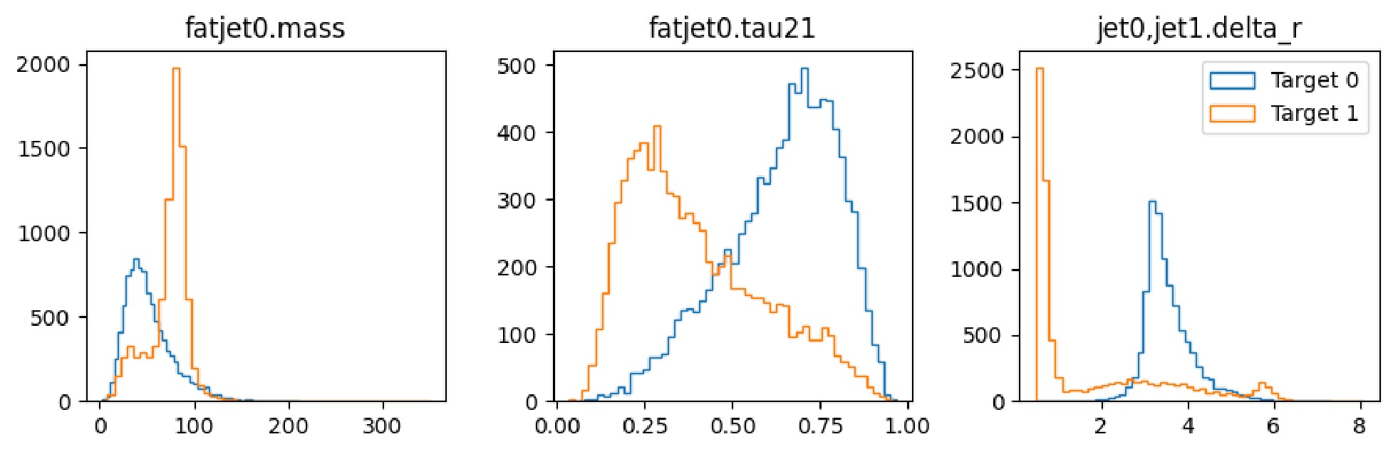

Figure 6.  (color online) Feature distributions of the set dataset.

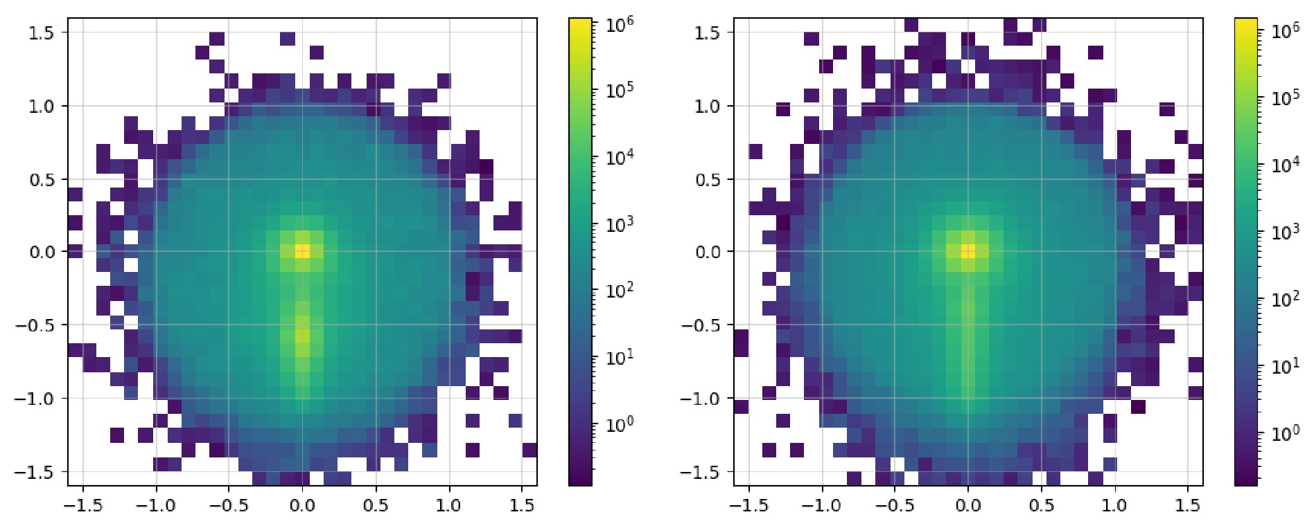
Figure 7.  (color online) Combined images of signal (left) and background (right) events.

Code example 32: Count the number of signals and backgrounds and show the distribution of the datasets.

It is observed that the number of signal and background instances is approximately equal, and the observables used clearly reflect the distinct characteristics of each, which is beneficial for our subsequent classification tasks. In the display of the image dataset, we show a merged image of the signal and background. It can be seen that the signal's fat jet image prominently features two sub-jets, whereas the sub-jets in the background are less distinct.

Once the datasets are prepared, let us import all available approaches for training. These approaches learn the differences between the signal and background. Subsequently, we use a dictionary and the built-in metrics to gather their performance, which will then be presented as a benchmark test. First, import all the necessary packages as 33, which we have roughly categorized to facilitate understanding of their purposes.

The selected evaluation metrics are accuracy, AUC (Area Under the Curve), signal significance, and background rejection rate at fixed signal efficiency. These metrics are commonly used in high-energy physics and help us better understand the approaches' performance. In code example 34, we define a function to retrieve the evaluation metrics of an approach.

For approaches, cut-and-count and the decision tree, they are not sensitive to the scale of features, so we can directly import the dataset (code example 35) and start training (code example 36). Two different topologies of the cut-and-count are taken to demonstrate how the order of applying cuts impacts performance.

Code example 33: Import necessary packages for the benchmark test.

Code example 34: Define a function to get the evaluation metrics of a model.

The input for the multilayer perceptron requires the use of $ \mathrm{MinMaxScaler}$ to scale the features within the 0-1 range, as detailed in code example 38, which aids in the model's rapid convergence. We train the model for 100 epochs with a batch size of 128. In code example 39, we illustrate the training process.

Code example 35: Load the set dataset for training cut-and-count and decision tree approaches.

Code example 36: Train the cut-and-count approaches with two different topologies.

Code example 37: Train the decision tree approach.

For the convolutional neural network, we employ two different preprocessing methods. One scales each image by its maximum value, while the other applies a logarithmic transformation to each pixel value. Given the large variations in pixel intensity in jet images, scaling directly by the maximum value might result in excessively small pixel values, whereas logarithmic transformation better preserves information. In code example 40 and 42, we load the image dataset and demonstrate these two distinct preprocessing techniques.

Code example 38: Load the set dataset for training the multilayer perceptron approach.

Code example 39: Train the multilayer perceptron approach.

Finally, we present a comparison of performance using code example 43. The results are shown in Table 3.

Name	ACC	AUC	Significance	R50	R99
${\mathrm{cnc}}\_{\mathrm{parallel}}$	0.750323	0.728121	33.660892	4.005174	1.000000
${\mathrm{cnc}}\_{\mathrm{sequential}}$	0.787784	0.769440	36.557026	4.712174	1.000000
$\mathrm{bdt}$	0.902011	0.955063	44.368549	117.804291	2.146139
$\mathrm{mlp}$	0.900904	0.956274	44.205276	117.804291	2.124265
${\mathrm{cnn}}\_{\mathrm{max}}$	0.806827	0.867769	38.444225	17.089737	1.188322
${\mathrm{cnn}}\_{\mathrm{log}}$	0.809452	0.876692	38.732323	19.042860	1.276514

Table 3.  Comparison of different approaches

From the significance column, we observe that for the cut-and-count method, the sequential topology, which considers the impacts among cuts, performs better than the parallel topology. For convolutional neural networks, the performance of logarithmic scaling is roughly equivalent to that using maximum value scaling. The multilayer perceptron and decision trees, which utilize features with clear distinctions, exhibit the best performance. For more practical problems, we can apply different approaches to the dataset and then select the most suitable one based on various performance metrics.

Code example 40: Load the image dataset and normalize the pixel values with the maximum value.

Code example 41: Train the convolutional neural network approach with the maximum value normalization.

In the current era where machine learning models are rapidly evolving, it is worthwhile to explore how to use them more conveniently in high-energy physics for searching new physical signals. In this paper, we introduce the $ \mathrm{hml}$ Python package, which offers a streamlined workflow from event generation to performance evaluation. The simplified process and control over random seeds significantly enhance the reproducibility of the final analysis results.

Code example 42: Normalize the pixel values by taking the logarithm. $ \mathrm{"..."}$ indicates the same code as in 40 and 41.

Code example 43: Compare the performance of different approaches.

We propose a naming convention for observables, which enables users to easily extract the required data from events output by DELPHES. Additionally, we extend the cut expression syntax originally in UPROOT to make it more user-friendly and compatible with DELPHES output formats. This convention is also utilized in our dataset construction process, helping users to quickly and conveniently build datasets. Based on this naming convention, we implement a transformation from the output of event generators to datasets usable by various analysis approaches. Moreover, the $ \mathrm{show}$ method included in datasets enables users to display data either as 1D distributions or 2D images, facilitating the adjustment of observable selections based on observed differences.

We have adopted the interface style of KERAS to standardize traditional methods such as the cut-and-count technique and decision trees. Furthermore, the cut-and-count approach supports automatic searching for the optimal cut positions, significantly reducing the workload for users. Additionally, we have incorporated commonly used evaluation metrics in high-energy physics, such as signal significance and background rejection rate at fixed signal efficiency. These metrics help users better understand the performance of the models.

We demonstrate the complete workflow through a practical example. It intuitively showcases the usage of $ \mathrm{hml}$. Currently, $ \mathrm{hml}$ is continuously being updated. We plan to incorporate more existing deep learning models, datasets, and extend to graph representations of data to further enhance its capabilities.