Note on single-trace EYM amplitudes with MHV configuration

In four dimensional spacetime, tree-level single-trace maximally-helicity-violating (MHV) amplitudes of Einstein-Yang-Mills (EYM) theory have been shown to satisfy the Selivanov-Bern-De Freitas-Wong [1−3] (SBDW) formula, which expresses the amplitude via a generating function. On another hand, Cachazo-He-Yuan (CHY) [4−6] formula gives a general approach to EYM amplitudes, which is independent of the dimension of spacetime and the helicity configuration. In four dimensions, the CHY formula has been shown to provide a spanning forest formula (first proposed in gravity, along the line of [7], [8] and [9]) for the single-trace MHV amplitude [10], which was further proven to be equivalent with the SBDW formula [10] and was generalized to double-trace MHV amplitudes [11] via the recursion expansion formula [12−16].

From another perspective, as pointed out in earlier literatures [17−21], each graviton in an EYM amplitude could be considered as a pair of collinear gluons which carry the same momentum and the same helicity. Particularly, inspired by the SBDW formula, [18] pointed out that the single-trace MHV amplitude with one and two gravitons can be explicitly expressed in terms of the MHV amplitudes where each graviton splits into a pair of collinear gluons [18]. This explicit formula of the single-trace MHV amplitudes was not extended into cases with an arbitrary number of gravitons yet. In this note, we take a small step forward in this direction: we provide a general formula for single-trace MHV amplitudes where each graviton splits into a pair of collinear gluons. When the number of gravitons is one or two, this formula turns back into the known results [18]. We hope this approach may provide a new insight for the study of helicity amplitudes in EYM.

The structure of this note is arranged as follows. In section 2, a helpful review of spinor-helicity formalism and the SBDW formula is presented. We study the amplitude with three gravitons in section 3 and sketch the general proof in section 4. Further discussions and conclusions are presented in section 5.

In this section, we provide a brief review of the spinor-helicity formalism in four dimensions [22], as well as the SBDW [1−3] formula and the spanning forest formula [10] for single-trace EYM amplitudes.

The momentum $ k^{\mu}_i $ of each on-shell massless particle i is expressed by two copies of Weyl spinors $ \lambda_i^{a}\widetilde{\lambda}_i^{\dot{a}} $. We define the spinor products as

where $ \epsilon_{{a}{b}} $ and $ \epsilon_{\dot{a}\dot{b}} $ are totally antisymmetric tensors. Apparently, the spinor products are antisymmetric objects under the exchanging of the two spinors. With this expression, the Lorentz contraction of two momenta $ k^{\mu}_a $ and $ k^{\mu}_b $ reads:

More helpful properties in spinor-helicity formalsim are displayed as follows.

● Momentum conservation for an n-point amplitude:

● Schouten identity:

● The eikonal identity resulted by Schouten identity

Finally, the n-gluon MHV amplitude $ A(1,...,n) $ at tree level satisfies the famous Parke-Taylor formula [23] ¹:

where i, j denote the two negative-helicity gluons and other gluons are supposed to be positive-helicity ones.

In EYM, there are two possible situations of the tree-level single-trace MHV amplitudes: the ($ g^-,g^- $) and ($ h^-,g^- $) configurations, which correspond to amplitudes with two negative-helicity gluons, and one negative-helicity gluon plus one negative-helicity graviton. In the following, we focus on the ($ g^-,g^- $) configuration. The ($ h^-,g^- $) can be studied similarly.

The SBDW [1−3] formula expresses the single trace ($ g^-g^- $)-MHV amplitude $ A(1,...,i,...,j,...,N|\mathrm{H}) $ in EYM as:

where 1,..., N are gluons arranged in a fixed ordering, $ \mathrm{H} = \{n_1,...,n_M\} $ are gravitons which are independent of color orderings. The negative-helicity gluons are supposed to be i and j. The $ S(i,j,\mathrm{H},\{1,...,N\}) $ factor is generated by an exponential generating function, particularly

in which

where $ \xi $, $ \eta $ are arbitrarily chosen reference spinors and G is the gluon set. In this note, we set $ \xi = 1 $ and $ \eta = N $ when studying the ($ g^-,g^- $) configuration.

It was shown in [10] that $ S(\mathrm{H};\mathrm{G}) $ could be expanded by spanning forest form. Particularly:

where we have summed over all possible forests F, where gluons and gravitons are considered as vertices, and the gluons are considered as the root set. Each edge $ ab $ is dressed by $ \psi_{ab} $, and multiply all such edges in a given forest F together.

In the case of ($ h^-,g^- $), the formulas (2) (3) and (5) are slightly changed [3, 10, 11] via (i). replacing $ i,j $ in (2) by the negative helicity graviton and the negative-helicity gluon, (ii). replacing the gravitons set H in (3) and (5) by the positive-helicity graviton set $ \mathrm{H}^+ $, while the root set is still the gluon set. (ii). introducing an extra minus $ (-1) $.

In this section, we extend the study of one and two graviton single-trace MHV amplitudes [18], where each gravition is presented as a pair of collinear gluons, to the cases with an arbitrary number of gravitons. We demonstrate this by the example with three gravitons in the current section, and then provide a general formula in the next section.

According to (2) and (5), the MHV amplitude with gluons 1,..., N and three gravitons $ n_1 $, $ n_2 $, $ n_3 $ is presented by

where $ S_3 $ is the abbreviation of the factor (5) with three gravitons. Specifically, $ S_3 $ is expressed as

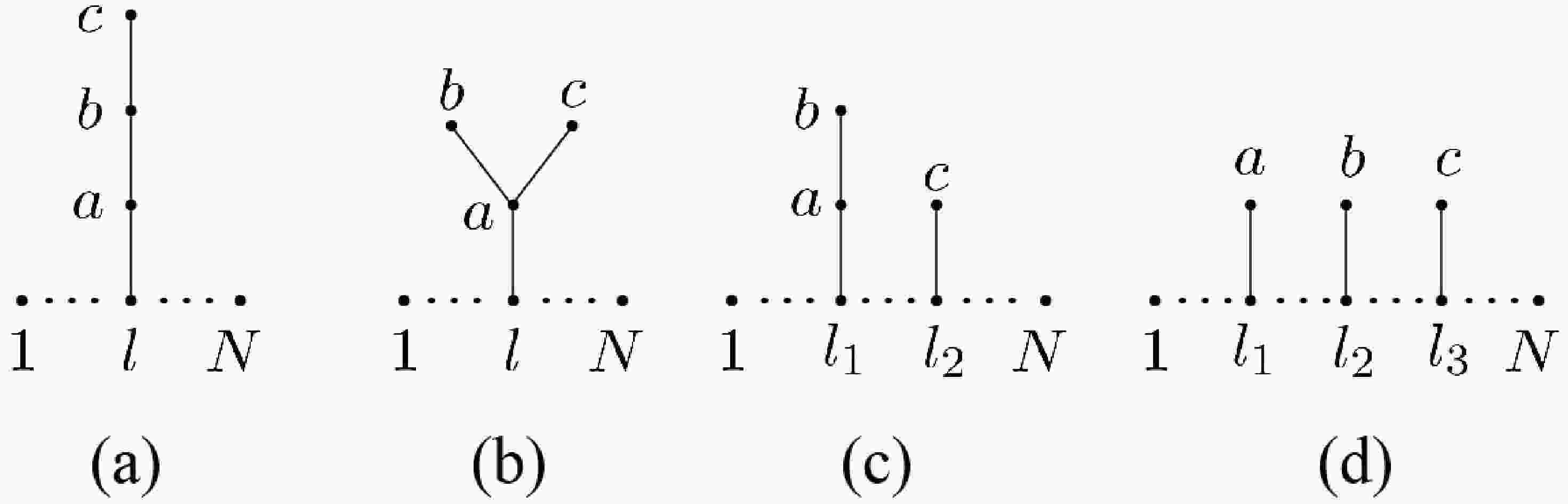
which are characterized by all possible spanning forests with structures Fig. 1. Each $ \psi_{ab} $ ($ a\neq b, a,b = 1,2,3 $) in the above expression is defined by (4) and is associating to an edge in the graphs Fig. 1, while the $ \psi_i $ ($ i = 1,2,3 $), associating to the graviton $ n_i $, is defined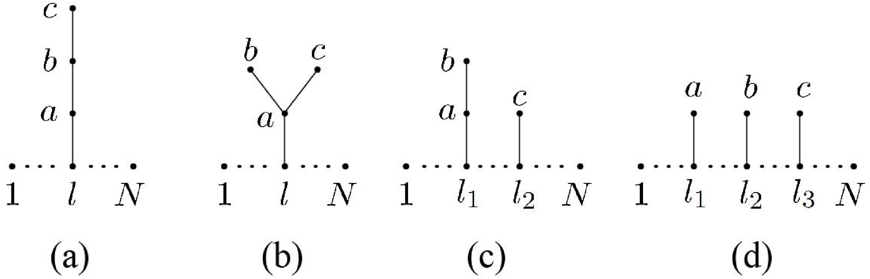 by

Figure 1.  All possible topologies of spanning forests for the three-graviton example. The a, b and c refer to different gravitons.

In the following, we analyze the contribution of each term in eq. (6).

First, let us deal with the term $ \psi_1\psi_{12}\psi_{23} $, which is characterized by Fig. 1 (a) (with $ a = 1 $, $ b = 2 $, $ c = 3 $), on the right hand side of eq. (6). Noting that

where the eikonal identity (1) and the fact that $ s_{ln_1} = [ln_1]\langle n_1l \rangle $ are applied, we write the Parke-Taylor factor accompanied by $ \psi_1\psi_{12}\psi_{23} $ as

where the factors $ \langle r_1,r_1+1\rangle $ and $ \langle t_1,t_1+1\rangle $ in the denominator of the Parke-Taylor factor have been replaced by $ \langle r_1,n_1\rangle\langle n_1,r_1+1 \rangle $ and $ \langle t_1,n_1\rangle\langle n_1,t_1+1 \rangle $, respectively. The $ n_1 $ in the second Parke-Taylor factor is further denoted by $ \widetilde n_1 $. Hence, the graviton $ n_1 $ splits into two gluons $ n_1 $ and $ \widetilde n_1 $ with the same momentum and helicity, which are respectively inserted between 1, l and l, N. Now we further express $ \psi_{12} $ and $ \psi_{23} $ by

respectively. When (9) is substituted into (8), we find that the graviton $ n_2 $ splits into two gluons $ n_2 $ and $ \widetilde n_2 $, which are respectively inserted to the left side of $ n_1 $ and to the right side of $ \widetilde n_1 $. Similarly, (10) finally inserts two gluons $ n_3 $ and $ \widetilde n_3 $ corresponding to the graviton $ n_3 $ to the left side of $ n_2 $ and the right side of $ \widetilde n_2 $. The term $ \dfrac{\langle ij\rangle^{4}}{\langle12\rangle\langle23\rangle\cdots\langle N1\rangle}\psi_1\psi_{12}\psi_{23} $ is then written as

in which, we introduced $ \text{PT}\left(a_1,...,a_m\right) $ to denote the PT factor $ \dfrac{\langle ij\rangle^{4}}{\langle a_1a_2\rangle\langle a_2a_3\rangle\cdots\langle a_ma_1\rangle} $ for short. Permutations $ {\boldsymbol{\rho}}^{(l)} $ for a given $ l\in\mathrm{G} $ are given by

where the $ A\shuffle B $ for two ordered sets A, B denotes all possible permutations by merging A and B together so that the relative ordering of elements in each of A and B is preserved. The above permutations can be characterized by the graph Fig. 2 (a).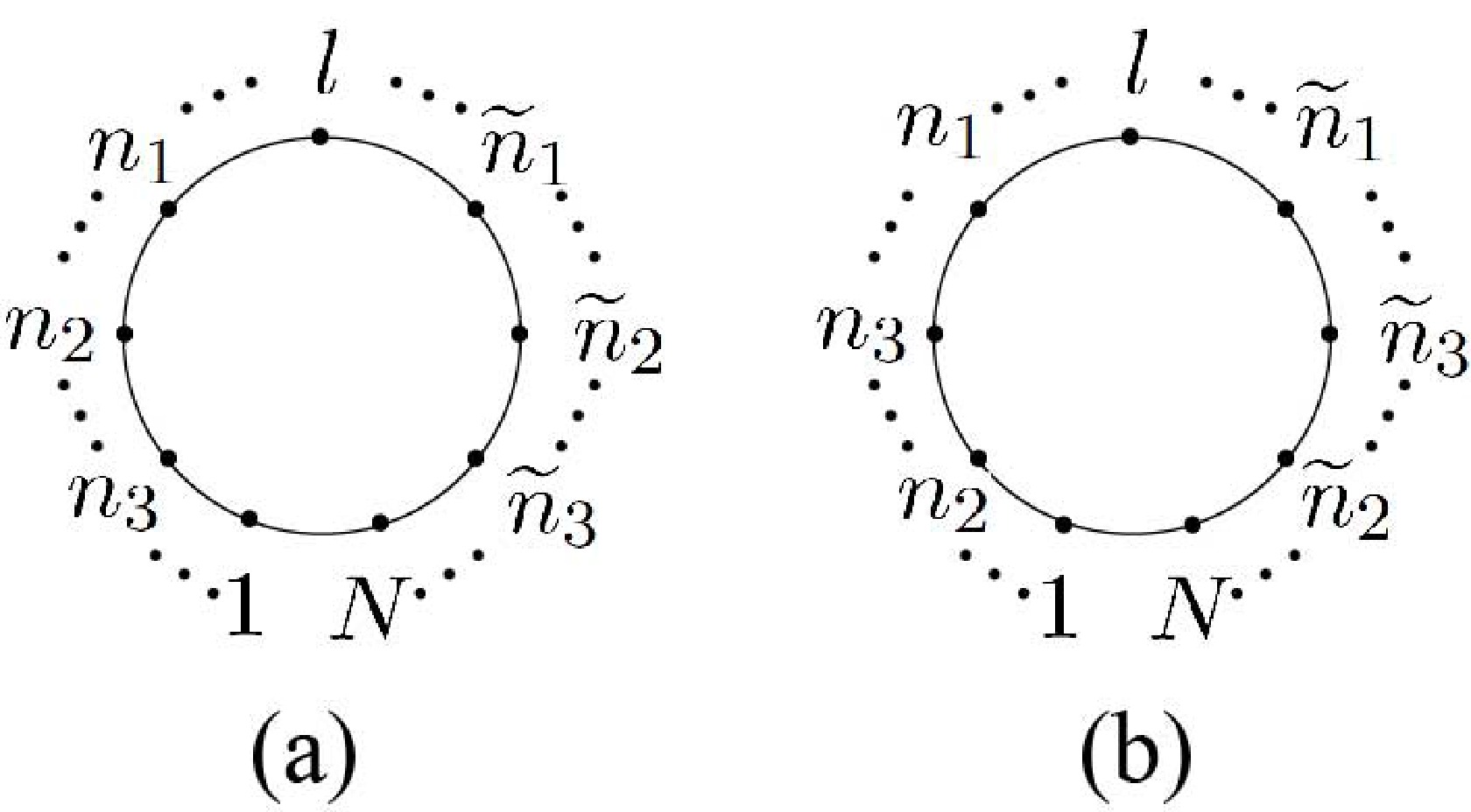

Figure 2.  (a). Permutations with the relative orderings $1,...,n_3,...,n_2,...,n_1,...,l,...,\widetilde n_1,...,\widetilde n_2,...,\widetilde n_3,...,N$. (b). Permutations with the relative orderings $1,...,n_2,...,n_3,...,n_1,...,l,...,\widetilde n_1,...,\widetilde n_3,...,\widetilde n_2,...,N$.

Second, we investigate the term with $ \psi_1\psi_{12}\psi_{13} $, which is associated to the graph Fig. 1 (b) (with $ a = 1 $, $ b = 2 $, $ c = 3 $). When the factor $ \psi_1 $ and $ \psi_{12} $ are expressed by (7) and (9), and $ \psi_{13} $ is expressed as follows

we just split the gravitons $ n_1 $, $ n_2 $ and $ n_3 $ into three pairs of gluons $ \{n_1,\widetilde n_1\} $, $ \{n_2,\widetilde n_2\} $ and $ \{n_3,\widetilde n_3\} $, respectively. The two gluons $ n_1 $, $ \widetilde n_1 $ coming from the graviton $ n_1 $ are inserted to the left and the right sides of l, while the $ n_2 $ and $ \widetilde n_2 $ (and also $ n_3 $ and $ \widetilde n_3 $) are further inserted to the left of $ n_1 $ and the right of $ \widetilde n_1 $. Thus this term turns into

where $ {\boldsymbol{\rho}}^{(l)} $ for a given l is now given by

which are characterized by Fig. 2 (a) and (b).

Third, we calculate the term with $ \psi_1\psi_{3}\psi_{12} $ (see Fig. 1 (c) with $ a = 1 $, $ b = 2 $, $ c = 3 $). When the same trick with the previous examples is applied, $ \psi_1 $ and $ \psi_{12} $ are expressed by (7) and (9), while $ \psi_3 $ is obtained via replacing $ n_1 $ in (7) by $ n_3 $. Again, these factors are used to insert gluon pairs into the Parke-Taylor factor. The result is

in which, $ {\boldsymbol{\rho}}^{(l_1,l_2)} $ for given $ (l_1,l_2) $ satisfies

On the second line, the $ {\boldsymbol{\rho}}^{(l_1)} $ denotes the permutations established by inserting the collinear gluons corresponding to $ n_1 $ and $ n_2 $ into the original gluon set, while $ {\boldsymbol{\rho}}^{(l_1)}_{L} $ and $ {\boldsymbol{\rho}}^{(l_1)}_{R} $ are the sectors separated by the gluon $ l_2 $ in the permutation $ {\boldsymbol{\rho}}^{(l_1)} $. Possible relative positions of $ l_2 $ in $ {\boldsymbol{\rho}}^{(l_1)} $ are displayed by Fig. 3 (a)-(g). Since the choices of $ l_1 $ and $ l_2 $ are independent of each other and we finally summed over all possible choices of $ l_1 $ and $ l_2 $, one can exchange the roles of $ l_1 $, $ l_2 $ in (12) as follows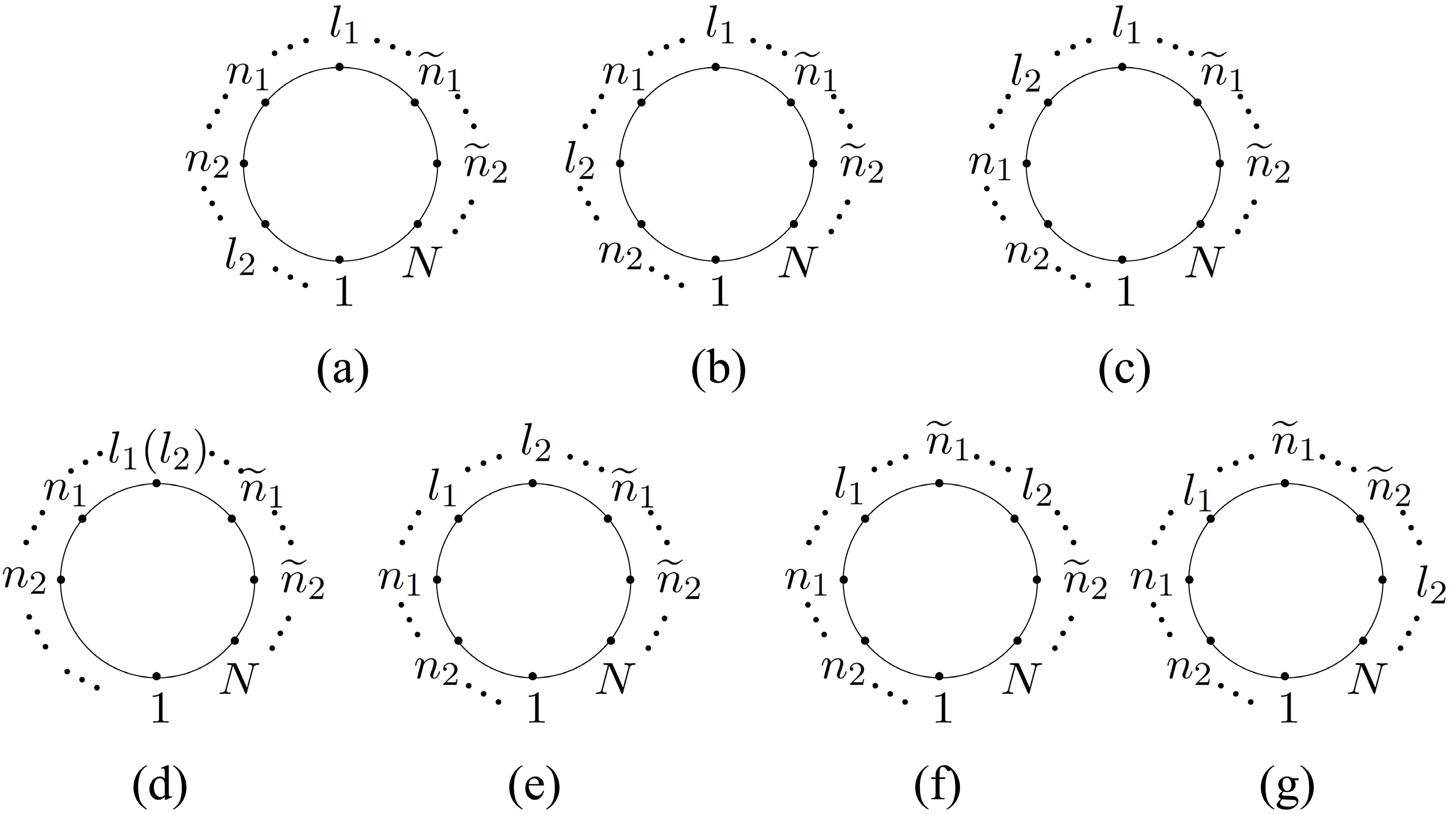

Figure 3.  Possible relative positions of $l_2$ in the permutations ${\boldsymbol{\rho}}^{(l_1)}$ in (12)

When all possible spanning forests for amplitude with three gravitons are considered, the full MHV amplitude with three gravitons is finally expressed by the following formula:

In the above expression, we have summed over all possible spanning forests where the original gluon set G plays as the root set. For a given spanning forest with i ($ i\leq 3 $) trees $ {\cal{T}}_1,...,{\cal{T}}_i $ planted at gluons $ l_1,...,l_i\in \mathrm{G} $ ($ l_j $ and $ l_k $ with distinct labels may be identical), each $ K({\cal{T}}_j) $ ($ j = 1,...,i $) is given by

where $ ab\in E({\cal{T}}_j) $ is an edge of the tree $ {\cal{T}}_j $ with vertices a and b. More explicity, there are four possible topologies for the three-graviton amplitude, as shown by Fig. 1 (a), (b), (c) and (d), which respectively provide factors

while a, b, c represent distinct gravitons. Two graphs with exchanging the branches attached to a same vertex are considered as the same graph, e.g. Fig. 1 (b). The permutations associated to Fig. 1 (a) and (b) can be recursively defined by (11) and (12), via replacing the subscripts 1, 2 and 3 of gravitons in (12) by a, b and c, respectively. The permutations for Fig. 1 (c) satisfy

Permutations accompanying to Fig. 1 (d) are presented by

Having displayed the example with three gravitons, we turn to the general formula in the next section.

Inspired by the example in the previous section, we propose the following general formula where gravitions split into pairs of collinear gluons

Here we sum over all possible spanning forests in which trees are planted at gluons $ l_1,...,l_i\in\mathrm{G} $. This summation is expressed by two summations:

● (i). summing over all possible choices of the roots $ l_1,...,l_i $ ($ i = 1,...,M $),

● (ii). for a given choice of roots $ l_1 $,..., $ l_i $, summing over all possible configurations of forests, which consist of nontrivial trees $ {\cal{T}}_1 $,..., $ {\cal{T}}_i $ planted at the gluons $ l_1 $,..., $ l_i $.

For a fixed forest, each tree $ {\cal{T}}_k $ is associated with a factor $ K({\cal{T}}_k) $ where each edge between two vertices a, b is assigned by a factor $ s_{ab} $. The permutations $ {\boldsymbol{\rho}}^{(l_1,...,l_k)} $ in the PT factors can be defined recursively:

where $ {\boldsymbol{\rho}}_L^{(l_1,...,l_{k-1})} $ and $ {\boldsymbol{\rho}}_R^{(l_1,...,l_{k-1})} $ denote the two ordered sets which are separated by the gluon $ l_k $ in the permutation $ {\boldsymbol{\rho}}^{(l_1,...,l_{k-1})} $. The $ {\boldsymbol{\sigma}}^{{\cal{T}}_k} $ ($ \widetilde{{\boldsymbol{\sigma}}}^{{\cal{T}}_k} $) stands for the permutations established by the tree graph $ {\cal{T}}_k $ whose nodes are $ \{n_i\} $ ($ \{\widetilde n_i\} $), while $ (\widetilde{{\boldsymbol{\sigma}}}^{{\cal{T}}_k})^T $ denotes the reverse of $ \widetilde{{\boldsymbol{\sigma}}}^{{\cal{T}}_k} $.

Now we sketch the proof of the general formula (15):

● (i). Step-1 Expand the MHV amplitude according to (2) and (5) in terms of spanning forests. Each forest F in general consists of i tree structures $ {\cal{T}}_1 $,..., $ {\cal{T}}_i $ planted to gluons $ l_1,...,l_i\in \mathrm{G} $.

● (ii). Step-2 For a given forest $ F = \{{\cal{T}}_1 $,..., $ {\cal{T}}_i\} $ and the tree $ {\cal{T}}_1 $, there are two types of edges (a). the edge between a graviton a and the root (a gluon $ l_1\in \mathrm{G} $), (b). The edge between two gravitons b and c. In the former case, the edge is associated with a factor $ \psi_{a} $ which is expressed according to (7), while an edge of the latter form is accompanied by a factor $ \psi_{bc} $, which is further rewritten as (9). After this manipulation, the factor $ \psi_{a} $ splits the graviton $ n_a $ into collinear gluons $ n_a $ and $ \widetilde n_a $ and then inserts them to the left and right of $ l_1 $, respectively. A factor $ \psi_{bc} $ splits the graviton $ n_c $ into collinear gluons $ n_c $ and $ \widetilde n_c $ which are further inserted to the left of $ n_b $ and the right of $ \widetilde n_b $ ($ n_b $ which is nearer to root than $ n_c $ has already been treated before). The factor assigned to each edge $ bc $ is $ s_{bc} $, and the product of all these factors gives $ K({\cal{T}}_1) $. The permutations established by this step are given by

● (iii). Step-3 Insert the collinear gluons corresponding to the gravitons on trees $ {\cal{T}}_2 $,..., $ {\cal{T}}_i $ in turn, by repeating step-2. We finally get the general formula (15) with permutations defined in (16).

In this note, we presented a formula (15) for single-trace EYM amplitudes in the MHV configuration (with two negative-helicity gluons). Each graviton in this formula splits into a pair of collinear gluons. Thus an N-gluon, M-graviton amplitude is finally expressed as a combination of $ N+2M $ gluon amplitudes with M pairs of collinear gluons. When the adjustment pointed in section 2 is considered, the formula (15) is straightforwardly extended to the MHV amplitude with one negative-helicity gluon and one negative-helicity graviton via (i). replacing i, j in the numerator of the PT factor by the negative-helicity graviton and the negative-helicity gluon, (ii). using the positive-helicity graviton set instead of the full graviton set on the RHS of (15). (iii). dressing the expression by an extra sign $ (-1) $. It is worth extending the collinear expression in the current paper to the double-trace amplitudes and amplitudes with other helicity configurations in a future work.