Off-equatorial deflections and gravitational lensing. II. In general stationary and axisymmetric spacetimes

The deflection of light rays in gravity has been extensively studied from the early stage of General Relativity [1, 2]. Today, gravitational lensing (GL) has developed into an effective tool in astronomy, ranging from measuring the mass of galaxies or their clusters [3], studying distributions of dark matter [4], investigating the properties of supernovas [5], to testing alternative gravitational theories [6, 7].

The simplest scenario of signal deflection and GL is that of light rays in static and spherically symmetric (SSS) spacetimes or in the equatorial plane of stationary and axisymmetric (SAS) spacetimes in the weak deflection limit (WDL). With the rapid development of astroparticle physics [8, 9], gravitational wave detection [10], and black hole (BH) imaging [11, 12], significant efforts have been devoted to the extension of the deflection and GL of timelike signals [13−18], with finite source and detector distance [19], and in the strong deflection limit [20−22]. Different analytical methods have also been developed, including perturbative methods [22−25] and the more recent Gauss-Bonnet theorem-based methods [16−18, 26].

However, extension to the non-equatorial deflection and GL in SAS spacetime is still rare (essentially non-equatorial motion does not occur in SSS spacetime), except in Kerr [27−33] and Kerr-Newmann (KN) [34, 35] spacetime. Owing to the complexity of the motion equations for off-equatorial trajectories, only a few works have studied deflection and GL in the quasi-equatorial motion of null rays [36, 37] or they have been studied only numerically in the general non-equatorial case [38, 39] in other spacetimes; neither has the deflection of both null and timelike rays been investigated. In Ref. [33], the general non-equatorial deflection and GL in Kerr spacetime were studied perturbatively for the first time for both null and timelike rays in the WDL, with the finite distance effect considered. One of the motivations of the current work is to study the condition under the form of SAS spacetime for the perturbative method to be feasible for non-equatorial deflection and GL. We show that for many SAS spacetimes satisfying a separation condition that enables a generalized Carter constant (GCC), the perturbative method is always valid for both null and timelike rays with the finite distance effect automatically considered. The second motivation is to reveal the effects of various spacetime parameters on such deflections and GL. The spacetimes being considered are the KN, Kerr-Sen (KS) [40], rotating Simpson–Visser (RSV) [41], and other spacetimes [42−45].

The remainder of this paper is organized as follows. In Sec. II A, we introduce the basic setup of the problem, establish the equations of motion, and study a condition for the perturbative method to work. In Sec. III, we explore a perturbative method to solve the deflection angle in both θ and ϕ directions. The off-equatorial GL equations are then solved in Sec. IV to obtain the apparent angles of the lensed images. In Sec. V, the method and deflection and GL results are applied to the KN, KS, and RSV spacetimes, and the effects of their characteristic parameters are studied. We conclude the paper with a summary and discussion in Sec. VI. Throughout the paper, we use the natural unit $ G = c = 1 $ and the spacetime signature ($ -,+,+,+ $).

In this section, we derive the deflection angles in the θ and ϕ directions for SAS spacetimes. We show that this is always possible when the metric functions satisfy certain conditions, such that a proper separation of variables in the equations of motion, or equivalently the existence of a GCC, can be accomplished.

We begin from the most general SAS spacetime, whose metric can always be expressed in the following form:

where $ t,\,r,\,\theta,\,\phi $ are the Boyer-Lindquist coordinates, and $ A,\,B,\,C,\,D,\,F $ are functions of r and θ only. This metric allows two commutative Killing vectors:

where the spacelike $ \psi^\mu $ corresponds to the rotation symmetry and timelike $ \xi^\mu $ to the time translation symmetry. These Killing vectors correspond to two conserved quantities of the motion:

Here, the dot denotes the derivative to the proper time or affine parameter λ of the motion, and E and L can be interpreted as the energy and angular momentum of the particle (per unit mass), respectively. In asymptotically flat spacetimes, E can also be related to the asymptotic velocity v of the particle through

The asymptotic velocity v is the magnitude of the spatial component of the four-velocity of the test particle. From these equations, we can obtain two first derivatives:

Now, for the equations of motion of the r and θ coordinates, we can simply express their geodesic equations. However, they are second-order equations that are very complicated to simplify. In this work, we will limit our choices of the SAS spacetimes, i.e., placing conditions on the metric functions, such that the motions enable a third conserved constant, i.e., the GCC [46]. We note that unlike the Kerr spacetime case, which not only contains a Carter constant [47] but even second-order Killing tensors [48], the existence of the GCC is not guaranteed in all SAS spacetimes. For those SAS spacetime without the GCC, many of them are non-integrable systems and even the geodesics are chaotic, such as Johannsen-Psaltis spacetime [49] and Zipoy-Voorhees spacetime [50]. We will not study these spacetimes in this work.

To observe the requirements of the existence of such a GCC and obtain (simpler) equations of motion for r and θ, we use the Hamiltonian-Jacobian approach. Our starting point is the action of the free particle for a separable solution, which is

where $ \kappa = 0,\,-1 $ for null and timelike particles, respectively. Here and hereafter, any function with an $ (r) $ or $ (\theta) $ superscript is a function of r or θ only. The Hamilton-Jacobi equation is given by

Substituting Eq. (7), this becomes

We then seek metrics that allow this equation, after being multiplied by a proper total factor function $ G(r,\theta) $, to be separable into r and θ dependent parts. This can be accomplished if the metric functions $ A,\,B,\,C,\,D,\,F $ and factor G can cast the left-hand sides of the following equations into their right-hand sides [46]:

where $ X\in\{A,\,B,\,C\} $. Note that the condition (10c) is for the separability of the $ \kappa = -1 $ case and unnecessary for null signals. Condition (10a) implies

In practice, the functions on the right-hand sides of Eq. (10) as well as $ G(r,\theta) $ can be obtained from the left-hand sides and Eq. (11). Additionally, a freedom of a multiplicative constant occurs in functions $ {\cal{D}}(r) $ and $ {\cal{F}}(\theta) $, and additive constant freedom occur in each pair of functions $ X^{(r)} $ and $ X^{(\theta)} $. Indeed, we can demonstrate that these freedoms will be canceled out in the final equations of motion (17) and (18) and therefore do not affect the physics. Moreover, many SAS spacetimes, including the Kerr spacetime, satisfy these conditions (10).

A few comments about the variable separation condition (10) might be useful for their clear understanding here. This work shows that the spacetimes satisfying condition (10) can always be treated using our method, whereas those spacetimes not satisfying (10) are not treatable using the method developed in this work. Hence, condition (10) is both a sufficient and necessary condition for the applicability of our method. However, Eq. (10) is only a sufficient condition for the separability of the equations of motion and we cannot prove that it is also a necessary condition, although we cannot provide any counter-example either. In other words, it is unclear to us whether spacetimes (unknown to us) exist that do not satisfy condition (10) but still allow the separation of its variables.

Using condition (10) in Eq. (9) and separating the r and θ dependent parts, we obtain

where the assigned constant K is the GCC we are searching for. Note that this GCC also allows some constants because we can always add or multiply a constant to both sides of the first equal sign in Eq. (12). However, these additive or multiplicative constants will not affect the dynamics; therefore, they can be selected freely. Thus, Eq. (12) can be split into two equations:

where we have defined two compact functions $ R(r) $ and $ \Theta(\theta) $ to simplify the notation. When the metric functions are known, these two functions can be determined. Therefore, functions $ S^{(r)} $ and $ S^{(\theta)} $ can be solved, and the action (7) becomes

where $ \pm_r $ and $ \pm_\theta $ are two signs introduced when taking the square roots in Eqs. (13) and (14). The motion equations for r and θ coordinates are determined using

to be

One of the main goals of this work is to determine the deflection angles of the trajectory in the WDL. Denoting the source and the detector coordinates as $ (r_s,\phi_s,\theta_s) $ and $ (r_d,\phi_d,\theta_d) $, respectively, this goal is equivalent to determining

In the WDL, we can reasonably assume that during the propagation of the signal, it experiences only one periapsis with radius $ r_0\gg M $, where M is the characteristic length scale of the spacetime, and one extreme value of the azimuth angle $ \theta_m $. i.e.,

The existence of such $ \theta_m $ means that it is either closer to 0 or π than both $ \theta_s $ and $ \theta_d $; therefore, we always have $ |\cos\theta_m|>|\cos\theta_{s,d}| $. From Eqs. (17) and (18), we observe that the above can be inverted to

After substituting Eqs. (13) and (14), this yields the more explicit relation

where

and $ s_2 = \pm 1 $ is introduced when solving a quadratic equation. These relations connect the motion constants $ (E,\,L,\,K) $ with $ (r_0,\,\theta_m) $. In Sec. III, we will use $ (r_0,\,\theta_m) $ to replace $ (L,\,K) $ because the latter are less intuitive and often more difficult to measure in astronomy. For example, $ r_0 $ for the bending by the Sun can be approximated using the solar radius.

To obtain the deflections $ \Delta\phi $ and $ \Delta\theta $, we first slightly transform the equations of motion (6), (17), and (18) and show that they can be integrated. First, from Eqs. (17) and (18), we easily find

which, after dividing $ G(r,\theta) $ and using Eq. (10a), yields

In contrast, substituting Eq. (10b) into Eq. (6), we have

After using Eqs. (10a) and (25), the r and θ dependent parts in this equation are separated:

Integrating Eq. (27), we directly obtain $ \Delta\phi $

Note that when integrating from $ r_s $ to $ r_0 $ (or $ r_0 $ to $ r_d $), the first term of Eq. (27) is expected to have $ \pm_r = -1 $ (or $ \pm_r = +1 $). When integrating from $ \theta_s $ to $ \theta_m $ (or $ \theta_m $ to $ \theta_d $), $ \pm_{\theta} = -1 $ (or $ \pm_{\theta} = +1 $) if $ \theta_m $ is a minimum or $ \pm_{\theta} = +1 $ (or $ \pm_{\theta} = -1 $) if $ \theta_m $ is a maximum. These sign values cause the extra $ s_1 = \mathrm{sign}(\cos(\theta_m)) $ sign in front of the second integral in Eq. (28). Similarly, by integrating Eq. (25), we obtain the following relation between initial and final θ coordinates:

This relation enales us to solve $ \theta_d $ when $ \theta_s $, the spacetime, and other kinetic variables are known. Therefore, from this, we can detremine the deflection in the θ direction as defined in Eq. (19).

The integrations (28) and (29), which solve the deflection angles, often cannot be used to obtain closed analytical forms. Therefore, in this section, we develop the perturbative method to approximate these integrals and then obtain the deflection.

The main concept of the perturbative method is selecting appropriate expansion parameter(s) and expanding the integrands into simpler series such that the integrations become executable. The WDL has a naturally small parameter $ 1/r_0 $ suitable for this purpose. When expanding the integrands in Eqs. (28) and (29), we can also anticipate that the expansion coefficients will explicitly depend on the asymptotic behavior of the metric functions. After a short survey of the applicable spacetime metrics of our method, we found the following expansions can be assumed for the functions $ X^{(\mu)} \; (\mu = r,\,\theta) $ and $ {\cal{D}}(r) $ and $ {\cal{F}}(\theta) $

where the constant a can be interpreted as the spacetime spin, and without losing any generality, we can always assume $ a\geq 0 $. Other coefficients $ a_n,\,b_n,\,c_n,\,d_n,\,g_n $ can be determined when the metric functions are known. Note that for the θ functions of the above form, the relation (20) between $ \theta_m $ and other parameters becomes very explicit as

and in principle, we can solve $ \theta_m $ in terms of other parameters if required. Substituting the above series and using the following simple changes of variables

in the integrals of Eqs. (28) and (29), we can further expand them with $ 1/r_0 $ as the small parameter into the following series forms:

where $ c_{s,d,m},\,s_{s,d,m} $, and the small dimensionless quantities $ p_{s,d} $ are defined as

The coefficients $ n_{r, i},\,n_{\theta, i},\,m_{r, i},\,m_{\theta, i} $ can be computed to any desired high order. Here, we only list their first few orders:

Some higher-order terms are presented in Appendix A. For the integrals over p in Eqs. (33) and (34), we can show that their integrands are always of the form $\text{polynomrial}(p)/ \left(1-p^2\right)^{n+1/2}\; (n = 0,\,1,\,\cdots)$ and therefore integrable [33]. For the integral over c in these equations, their integrands are always of the form $\text{polynomrial}(c)/ \left[(1-c^2)^n \sqrt{c_m^2-c^2}\right]\; (n = 0,\,1)$ and therefore also integrable.

The results of the integrations are of the form

where $ N_{r,i},\,N_{\theta,i},\,M_{r,i},\,M_{\theta,i} $ are the corresponding integral results of the $ n_{r,i},\,n_{\theta,i},\,m_{r,i},\,m_{\theta,i} $ terms. Again, the first few terms are

and some higher-order results are given in Appendix A.

We note that the deflection $ \Delta\phi $ in Eq. (36) still contains the unknown $ \theta_d $ in its second term coefficients $ N_{\theta,i} $. In contrasat, Eq. (37) effectively establishes a relation between $ \theta_d $ (or $ \cos\theta_d $) and other parameters. Therefore, to solve the deflections $ \Delta\phi $ and $ \Delta\theta $, we must first solve $ \cos\theta_d $ from Eq. (37). In the WDL, $ \cos\theta_d $ can also be expressed in the series form

where the coefficients $ h_i $ are solvable from Eq. (37) using the method of undetermined coefficients. Here, we only show the first two orders:

and higher order ones are given in Appendix A.

Substituting Eq. (39) into Eq. (36) and performing the small $ 1/r_0 $ expansion again, we finally determine the deflection $ \Delta\phi $ as

where $ N_{r,i} $ is unchanged as in Eq. (38), and the first few $ N^\prime_{\theta,i} $ values are

Inspecting the above results, we discover that $ s_2 $ is simply the sign of $ \Delta\phi $ at the lowest order, which also means that $ s_2 = \pm1 $ correspond to anticlockwise and clockwise motions, respectively. Naturally, the following relation holds:

In the infinite $ r_{s,d} $ limit, we observe clearly from the $ N^\prime_{\theta,0} $ term that $ \Delta\phi $ to the leading order equals $ s_2\pi $.

Similarly, substituting (39) into Eq. (19), the deflection in θ direction becomes

where

Note that in the limit $ r_{s,d}\to\infty $, $ h_0 $ approaches $ -c_s $; therefore, $ k_0 $ approaches 0.

Eqs. (41) and (44) are two important results of this work, and a few comments are necessary concerning them. First, these results apply to general SAS spacetimes that allow the existence of a GCC. This includes many well-known spacetimes such as the Kerr, KN, and all SSS apacetime, which can be obtained by setting all $ b_n = 0 $ for $ n\geq2 $. Second, they apply to both light rays (setting $ \kappa = 0 $) and timelike particles (setting $ \kappa = -1 $). Indeed, we can show that the $ E\to\infty $ limits of these results for timlike signals equal exactly their values for null rays. Third, these deflections also consider the finite distance effect of the source and detector. This effect can be important when studying the GL effect. Through setting $ p_{s,d} $ to zero, the infinite distance version of the deflections can be obtained. Fourth, these deflections apply to both non-equatorial and equatorial trajectories. For the former, setting $ \theta_{s,d}\to \pi/2 $, we have verified that the deflection angle $ \Delta\phi $ reduces to its value on the equatorial plane in the Kerr spacetime [23]. For the latter, these formulas do not rely on any near-equatorial plane approximation, i.e., $ \theta_s $ and $ \theta_d $ can be far from $ \pi/2 $. Last but not least, the deflections (41) and (44) can be further expanded around small $ p_{s,d} $ values if the source and detector are far away, i.e., $ r_{s,d}\gg r_0 $, and a dual series form will be obtained. Such a form will be more appealing from the application perspective, and we explore this in Sec. V.

As we have obtained the deflection angles for arbitrary inclination angles of the signals, we can study GL in such SAS spacetime in the off-equatorial plane. Because our deflection angles (41) and (44) contain the finite distance effect, we can naturally establish the following GL equations:

Here, $ \delta\phi $ and $ \delta\theta $ are the two small angles characterizing the angular position of the source relative to the detector-lens axis in the spherical coordinates, as shown in the schematic diagram in Fig. 1. When $ r_{s,d},\,\theta_s $ are fixed, then substituting Eqs. (41) and (44) into Eq. (46) enables us to solve the minimal radius and extreme azimuth angle $ (r_0,\,\theta_m) $ for each pair of $ \delta\phi,\,\delta\theta $. However, Eqs. (46) are high-order polynomials of $ r_0 $ and more complicated functions of $ \theta_m $, which often cannot be solved analytically, particularly when the effects of higher-order parameters are sought. Therefore, we often use the numerical method to solve them.

Figure 1.  Schematic diagram of one trajectory from the source at ${\rm{S}} (r_s,\,\phi_s,\,\theta_s) $ to the detector at $ {\rm{D}}(r_d,\,\phi_d,\,\theta_d) $. $ r_0 $ and $ \theta_m $ mark the minimal radius and extreme θ points on the trajectory, respectively. $ (\alpha,\,\beta) $ marks the apparent angle formed by this trajectory on the celestial sphere of the observer.

Generally, two sets of $ (r_0,\,\theta_m) $ enable the signal to reach the detector. When the deflection $ (\delta\theta,\,\delta\phi) $ is not small, these two solutions will often have opposite orbital rotation directions $ s_2 $, and the $ s_1 = \mathrm{sign}(\cos(\theta_m)) $ equals $ s_2 $ for each solution. Only when the source, lens, and detector are aligned (deflection less than $ 10^{-6\prime\prime} $ in the Sgr A* scenario considered in Sec. V A) and the spacetime spin is large could exceptions exist (see also Ref. [33]). Therefore, we label these two solutions as $ (r_{0+},\,\theta_{m+}) $ and $ (r_{0-},\,\theta_{m-}) $ to represent the prograde and retrograde rotating signals, respectively. In this paper, by prograde and retrograde, we mean that the trajectories are rotating anticlockwise and clockwise around the $ +\hat{z} $ directions, respectively. No retrolensing is involved because we discuss only the weak deflection cases.

However, to link the solved $ (r_0,\,\theta_m) $ to the observables of the GL, we must still determine the formula for the apparent angles of the lensed images. For a static observer in the spacetime with metric (1), the associated tetrad $ (e_a)^\mu $ takes the form

where Z is the four-velocity of the observer. Thus, for a signal with four-velocity $ u^\mu = (\dot{t},\,\dot{\phi},\,\dot{r},\,\dot{\theta}) $, its projection using the projection operator $ h^\mu_{\ \nu} = \delta^\mu_{\ \nu}+Z^\mu Z_\nu $ into the tetrad frame yields the vector

Here, $ (\dot{r},\,\dot{\theta},\,\dot{\phi}) $ are linked to $ (L,\,K) $ through Eqs. (6), (17), and (18) and then to $ (r_{0\pm},\,\theta_{m\pm}) $ through Eqs. (22) and (23). Thus, the apparent angle $ \gamma_\pm $ measured by this observer against the detector's radial direction $ \hat{r}_d $ and $ \alpha_\pm $ against the $ \hat{r}_d\hat{\theta}_d $ plane and $ \beta_\pm $ against the $ \hat{r}_d\hat{\phi}_d $ plane are, respectively,

where the subscript $ |_d $ means that all coordinates should be evaluated at the detector location. These equations are valid for all trajectories in the SAS spacetimes, including those that are bent strongly. In the large $ r_d $ limit, $ \gamma_\pm^2\approx \alpha_\pm^2+\beta_\pm^2 $; therefore, we must focus on two of them, which are conventionally selected as $ (\alpha_\pm,\,\beta_\pm) $.

In this section, we apply the general method and the results in Secs. III and IV to some known SAS spacetimes to examine the validity of the results and significance of the spacetime parameters on the off-equatorial deflection and GL. We focus on deflections $ \Delta\phi,\,\Delta\theta $, the $ r_0,\theta_m $ and apparent angles $ \alpha_\pm,\,\beta_\pm $.

For the KN BH, the deflection in its equatorial plane has been considered using analytical methods repeatedly, and the (quasi-)equatorial motion, as well as numerical solutions of the trajectories, has also been studied multiple times [51−55]. However, to our best knowledge, the perturbative study of the general off-equatorial deflection has not been conducted yet.

The metric of KN is given by

where

and $ M,\, Q,\,a = J/M $ are the mass, charge, and spin angular momentum per unit mass of the spacetime, respectively. In studying the trajectories, we can always select $ a\geq0 $ if the motion is allowed to go both clock- and anticlock-wise. To use the method and results developed in Secs. III and IV, we must first check whether the metric (50) satisfies the separation requirements (30). Substituting the metric into these equations, we easily observe that the separation can be performed, and the r-dependent functions are

and $ X^{(\theta)}\; (X\in\{A,\,B,\,C,\,{\cal{F}},\,G\}) $ are exactly as given in Eq. (30). This guarantees the existence of the GCC, as was well-known prior, and the applicability of the results of deflection angles.

Substituting the coefficients in Eqs. (51) directly into Eq. (41) and (44) and performing the small $ p_{s,d} $ expansion, the deflection angles in KN spacetime are determined as dual series of $ M/r_0 $ and $ p_{s,d} $

where the infinitesimal $ \epsilon $ represents either the $ M/r_0 $ or $ p_{s,d} $, and

$ \hat{a}\equiv a/M,\,\hat{Q}\equiv Q/M, $ and E has been replaced by the asymptotic velocity v through Eq. (4). We can take a few limits for these deflections. Through setting $ v = 1 $ or $ p_{s,d} = 0 $, they reduce to deflections of light rays or deflections from infinity to infinity, respectively. A more unusual limit is to set $ \hat{a} = 0 $, which pushes these deflections to their values of the signal in an RN spacetime but with an arbitrary incoming direction. For $ \hat{Q} = 0 $, they agree with Eqs. (32) and (39) of Ref. [33]. In the infinite distance and equatorial limit, $ p_s,\,p_d,\,c_m,\,c_s\to 0 $ and $ s_m,\,s_s\to 1 $, and we have checked that $ \Delta\phi_{\mathrm{KN}} $ in this limit agrees with Eq. (83) of Ref. [24].

Both Eqs. (52a) and (52b) illustrate various effects of the non-equatorial motion and spacetime parameters. For the deflection $ \Delta\phi_{\mathrm{KN}} $, the following observations can be made. First, we observe that the non-equatorial effect manifests in two ways. The first is through the terms proportional to $ c_s\sqrt{c_m^2-c_s^2} $. These terms will vanish in the equatorial limit; therefore, we call them non-equatorial terms. The second way of the non-equatorial effect is through the factor $ s_m^n/s_s^2 $ of the other terms, which will be called the equatorial terms. If the trajectory were in the equatorial plane, these factors would all be one. Therefore, these factors effectively adjust the contribution of equatorial terms to the deflection. The second comment concerns the effects of the spacetime charge and spin. For equatorial motion, $ \hat{Q} $ and $ \hat{a} $ begin to appear in the equatorial terms from the second order only, i.e., the $ (M/r_0)^2,\,(r_0/r_{s,d})^2 $ or $ (M/r_0)(r_0/r_{s,d}) $ terms. While in non-equatorial terms, they begin to appear from the third order.

The terms of the deflection $ \Delta\theta $ in Eq. (52b) are either proportional to $ \sqrt{c_m^2-c_s^2} $ or $ c_s $, which both approach zero in the equatorial limit. At the leading orders of both $ (M/r_0) $ and $ p_{s,d} $, the terms are proportional to $ \sqrt{c_m^2-c_s^2} $. For the effect of both $ \hat{Q} $ and $ \hat{a} $, they both appear from the second order, which is similar to the equatorial terms in $ \Delta\phi_{\mathrm{KN}} $. In both $ \Delta\phi_{\mathrm{KN}} $ and $ \Delta\theta_{\mathrm{KN}} $, the sign of $ \hat{Q} $ does not matter, as expected because the signal is neutral.

To check the validity of these deflections (52a) and (52b), in Fig. 2 we compare them with their corresponding numerically integrated values. In this plot, we select a relatively small $ r_0 $ such that the deflections are appreciable to tell the effects of various parameters. We observe in Fig. 2 (a) and (b) that as $ r_0 $ increases, both $ |\Delta\phi_{\mathrm{KN}}| $ and $ |\Delta\theta_{\mathrm{KN}}| $ decrease monotonically. The analytical results approach the numerical value more closely as $ r_0 $ increases, which is expected because both deflections are series of $ (M/r_0) $. From Fig. 2 (c) and (d), we observe that as $ \theta_m $ decreases, the deflection in the θ direction increases, whereas that in the ϕ direction decreases. This is intuitively consistent with the physical expectation because the decrease in $ \theta_m $ corresponds to the motion of the trajectory asymptotic line towards the z axis above the equatorial plane. Fig. 2 (e) shows the effect of $ \hat{Q} $ on the deflections. Previously, the equatorial plane case implied that $ |\Delta\phi_{\mathrm{KN}}| $ would decrease as $ \hat{Q} $ increases [55], which is still observed here for the off-equatorial motion. We also note that this is even true for $ \Delta\theta_{\mathrm{KN}} $, which shows the spherical nature of the effect of $ \hat{Q} $ on the deflections. Finally, the effect of the spacetime spin $ \hat{a} $ on these deflections was studied in Ref. [33] in the Kerr spacetime, and we found that the effect is not changed qualitatively: a larger $ \hat{a} $ increases (or decreases) the $ \delta\phi $ of the prograde (or retrograde) signal.

Figure 2.  (color online) Dependences of $ \Delta\phi $ and $ \Delta\theta $ on $ r_0,\,\theta_m $ and $ \hat{Q} $ in KN spacetime. $ v = 1,\,r_s = r_d = 400M, $$ \,\hat{a} = 1/2,\,\theta_s = \pi/4 $. In (a)(b), $ \hat{Q} = 1/2 $, $ \theta_m = \pi/5 $. In (c)(d), $ \hat{Q} = 1/2,\,r_0 = 20M $. In (e), $ r_0 = 20M,\,\theta_m = \pi/5 $. All red lines represent numerical results.

With the correctness of the series results confirmed, we can now solve the lensing equations (46) with $ \Delta\theta $ and $ \Delta\phi $ given by Eqs. (52b) and (52a) to obtain the $ (r_0,\,\theta_m) $ for a fixed pair $ (\delta\phi,\,\delta\theta) $ that characterizes the angular deflection of the source against the lens-observer axis. For the non-equatorial motion in a SAS spacetime, the source's azimuth angle $ \theta_s $ also becomes important. Because these equations are high-order polynomials if the effects of $ \hat{Q} $ and $ \hat{a} $ are considered, we have only solved them numerically. We used the Sgr A* BH as the lens and set $ r_d = r_s = 8.34\; \mathrm{kpc} $ and varied $ (\delta\phi,\,\delta\theta,\,\theta_s) $. We found that, qualitatively, the effects of $ \delta\phi,\,\delta\theta,\,\theta_s $, and $ \hat{a} $ are similar to their effects in the Kerr case studied in Ref. [33]. Therefore, we will not show these figures here. Instead, we only mention that a larger positive $ \hat{a} $ decreases (or increases) the $ r_0 $ of a counterclockwise (or clockwise) rotating trajectory; therefore, the trajectory is pulled towards (or pushed away from) the z axis. $ \theta_m $ will change accordingly: a larger positive $ \hat{a} $ will increase $ |\cos\theta_m| $ of both counterclockwise and clockwise rotating orbits. For the charge $ \hat{Q} $, its deviation from zero decreases $ r_0 $ for all $ \hat{a} $ and orbit rotation directions and increases $ |\cos\theta_m| $ very weakly.

Finally, substituting the solved $ (r_0,\,\theta_m) $ together with the initial parameters $ (\delta\theta,\,\theta_s,\,r_d) $ into Eqs. (49b) and (49c), we can obtain the apparent positions of the two images on the celestial sphere of the detector:

where $ \Theta_\pm $ is defined in Eq. (14) and takes the form

in KN spacetime. $ L_\pm,\,K_\pm $ can be fixed by $ (r_{0\pm},\,\theta_{m\pm}) $ through Eqs. (22) and (23). These apparent angles are consistent with the results in Ref. [33]. For the null particle in the WDL, we can make the following power series approximation by taking $ M/r_0 $ and $ M/r_d $ as small quantities:

where and henthforce $ \hat{r}_{0\pm}\equiv r_{0\pm}/M,\; \hat{r}_d\equiv r_d/M,\; s_{m\pm} = \sin\theta_{m\pm} $. When we set $ \hat{Q} = 0 $, they agree with Ref. [33]. However, when $ \hat{Q}\neq0 $, its effect does not only appear from the $ Q^2/(r_{0\pm}r_d) $ order as we might think superficially from Eq. (56). Indeed, $ \hat{Q} $ affects $ \hat{r}_{0\pm} $ by an amount similar to the size of $ \hat{Q} $ itself; therefore, its influence on the image apparent angles is at the $ Q/r_d $ order, i.e., one order lower than what appears in Eq. (56). The off-equatorial effect influences $ \gamma_{\pm\mathrm{KN}} $ from the second order because, at the leading order, the total apparent angle $ \gamma_{\pm\mathrm{KN}}\approx\sqrt{\alpha_{\pm\mathrm{KN}}^2+\beta_{\pm\mathrm{KN}}^2} $ would not be tuned by the factor $ s_{m\pm}/s_d $ or $ \sqrt{s_d^2-s_{m\pm}^2}/s_d $ in front of $ \alpha_{\pm\mathrm{KN}} $ and $ \beta_{\pm\mathrm{KN}} $, respectively.

In Fig. 3, the angular positions of the GL images as functions of $ \delta\phi $ (a) and $ \delta\theta $ (b) are plotted. It is seen that as $ \delta\phi $ varies from $ 0 $ to $ 10^{\prime\prime} $ while keeping $ \delta\theta $ at $ 1^{\prime\prime} $, the two images are in the first and third quadrants, respectively. The image in the third quadrant is separated further from the lens than the one in the first quadrant. Because in this parameter settings, the effect of spin $ \hat{a} $ on the apparent angles of the images is weak, when we flip $ \delta\phi $ to the range of $ -10^{\prime\prime} $ to 0, or $ \delta\theta $ to $ -1^{\prime\prime} $, the images are reflected by the y and x axes, respectively, in the 2d celestial frame. More interesting is the effect of $ \theta_s $ in this plot. The trace of the images as $ \delta\phi $ varies for $ \theta_s = \pi/6 $ almost coincides with that for $ \theta_s = \pi/3 $. The reason can be understood from the fact that when the spin $ \hat{a} $ effect is not strong, the total deflection in an SAS spacetime is approximately the same as that in an SSS spacetime. In SSS spacetimes, $ \theta_s $ characterizes only the altitude of the images, whereas, when $ \delta\phi $ scans through a range, the traces of the images will coincide if the origin of the local 2d celestial sky is allowed to shift, as in Fig. 3 (a). For the variation in $ \delta\theta $ with fixed $ \delta\phi = \pm 1^{\prime\prime} $, different $ \theta_s $ values enable a different contribution from $ \delta\theta $ to the total deflection $ \delta\eta $, which roughly equals

Figure 3.  (color online) Apparent angles of lensed images in the celestial sky in KN spacetime. (a) $ \delta\phi $ varies from $ -10^{\prime\prime} $ to $ 10^{\prime\prime} $ with fixed $ \delta\theta = 1^{\prime\prime} $ ($ \Box $ and $ \times $) and $ -1^{\prime\prime} $ ($ \circ $ and $ + $). (b) $ \delta\theta $ varies from $ -10^{\prime\prime} $ to $ 10^{\prime\prime} $ with fixed $ \delta\phi = 1^{\prime\prime} $ ($ \Box $ and $ \times $) and $ -1^{\prime\prime} $ ($ \circ $ and $ + $). The symbols $ \Box $ and $ \circ $ are for $ \theta_s = \pi/3 $ and $ \times $ and $ + $ are for $ \theta_s = \pi/6 $. The color of the symbols from blue to red indicates that the changing angles increase from $ -10^{\prime\prime} $ to $ 10^{\prime\prime} $. (c) Variation in the apparent angles as $ \hat{Q} $ increases. In all plots, $ \hat{a} = \hat{Q} = 1/2,\,v = 1,\,M = 4.1\times 10^6M_\odot, $$ \,r_s = r_d = 8.34 $ kpc are used. In (c), $\delta \theta = 10^{-4\prime\prime},\,\delta \phi = 10^{-4\prime\prime}, $$ \,\theta_s = \pi/6$. The $\alpha_{0+} = 0.60780640^{\prime\prime},\,\alpha_{0-} = -0.60783265^{\prime\prime},\,\beta_{0+} = $$ 1.2776103^{\prime\prime}, \beta_{0-} = -1.2776603^{\prime\prime}$.

and, therefore, the image traces will not coincide, as shown in Fig. 3 (b).

Note that in both plots, we have set $ \hat{a} = 1/2,\,\hat{Q} = 1/2 $. The effect of these parameters under the current parameter settings, as observed from Eq. (56), is very small compared with the apparent angles themselves. Thus, they cannot be recognized in plots (a) and (b). Therefore, in (c), we show the small variation in the apparent angles $ (\alpha_{\pm \mathrm{KN}},\,\beta_{\pm \mathrm{KN}}) $ as $ \hat{Q} $ increases, where $ \alpha_{0\pm} = \alpha_{\pm\mathrm{KN}}(\hat{Q} = 0) $, $ \beta_{0\pm} = \beta_{\pm \mathrm{KN}}(\hat{Q} = 0) $. The sizes of the apparent angles of both images decrease by about $ 10^{-6\prime\prime} $ as $ \hat{Q} $ increases. Both the trend and changed amount agree with the prediction of Eq. (56).

The KS BH is a type of rotating and charged BH in the four-dimensional heterotic string theory [40]. Although both the strong [56] and weak [36] deflection limits of GL effects have been studied in this spacetime using approaches different from ours, these studies focused either on the (quasi-)equatorial plane or did not express the deflections in terms of the original source and kinetic variables. Here, we extend them to the general non-equatorial case and consider the finite distance and timelike effects.

The metric of the KS spacetime is given by [57]

where

with $ b\equiv Q^2/(2M)\geq0 $. This metric reduces to the Kerr spacetime when $ b = 0 $. The metric functions also satisfy the separation conditions (10), and the corresponding functions and their asymptotic expansions are

Substituting the coefficients Eqs. (59) into Eqs. (41) and (44) and performing the small $ p_{s,d} $ expansion, we determine the deflection angles in KS spacetime as

where

and $ \hat{b}\equiv b/M $. Comparing Eq. (60) with the corresponding results in Eq. (52) in KN spacetime, we observe that the only change is essentially in the definition of $ \zeta_\mathrm{KS} $. This is understandable because both the KN and KS spacetimes reduce to the Kerr one if we set $ Q = 0 $ in the former and b (or Q) in the latter, and these two parameters only appear from the second order in each of the deflections $ \Delta\phi $ and $ \Delta\theta $. The infinite source/detector and null limits of the deflections (60) can be easily obtained by setting $ v = 1 $ and $ p_{s,d} = 0 $. The equatorial plane case of $ \Delta\phi $ was determined in Eq. (49) of Ref. [56] for a light ray and infinite source/detector and agrees with our result under these limits.

To study the effect of the new parameter $ \hat{b} $ on the deflections, in Fig. 4 (a) we plot the dependence of $ \Delta\phi_\mathrm{KS} $ and $ \Delta\theta_\mathrm{KS} $ on $ \hat{b} $. As $ \hat{b} $ increases, both deflections $ \Delta\phi_\mathrm{KS} $ and $ \Delta\theta_\mathrm{KS} $ for all spin $ \hat{a} $ decrease monotonically. This effect is qualitatively similar to the effect of $ \hat{Q}^2 $ in KN spacetime.

Figure 4.  (color online) Dependences of $ \Delta\phi $ and $ \Delta\theta $ (a) and α and β (b) on $ \hat{b} $ in KS spacetime: (a) v = 1, $ \hat{a} $ = 1/2, $ r_s = r_d = 400M,\,\theta_s = \pi/4,\,\theta_m = \pi/5,\,r_0 = 20M$; (b) v = 1, $\,\hat{a} = $$ 1/2,\;M = 4.1\times 10^6M_\odot,\;r_s = r_d = 8.34\; \mathrm{kpc},\; \delta \theta = 10^{-4\prime\prime},\; \delta \phi = 10^{-4\prime\prime},\;\theta_s = \pi/6.$

With the deflection known, we can solve the GL Eq. (46) for $ r_0 $ and $ \theta_m $. Again, if we use the deflection angles of sufficiantly high order such that the effect of $ \hat{b} $ is considered, these GL equations are polynomials whose solutions are too lengthy to present here and therefore we will not do so. We also studied the dependence of the solved $ (r_0,\,\theta_m) $ on $ \hat{b} $ and found that it is also qualitatively similar to the effect of $ \hat{Q}^2 $ in KN spacetime. That is, $ r_0 $ decreases as $ \hat{b} $ increases for fixed $ \hat{a} $, whereas $ |\cos\theta_m| $ increases but only very weakly in the WDL.

Using these $ r_0 $ and $ \theta_m $ in Eq. (49), we determine the apparent angles in the KS spacetime as

where $ \Theta_\pm $ in the KS spacetime also takes the form of Eq. (55) but its $ (L_\pm, \,K_\pm) $ have different relations to $ (r_{0\pm},\,\theta_{m\pm}) $ through Eqs. (22) and (23). For null rays and the small $ M/r_0 $ and $ M/r_d $ limit, these apparent angles are approximated as

In contrast to the parameter $ \hat{Q} $ in the KN apparent angles (56), we observe that the parameter $ \hat{b} $ affects the apparent angles in KS spacetime from the order $ b/r_d $ explicitly. However, we also indicate that as $ \hat{b} $ increases from zero, its influence on $ r_{0\pm} $ is also at this order but slightly larger and with an opposite sign.

Figure 4 (b) shows the apparent locations of the images in the KS spacetime as $ \hat{b} $ varies. The $ \alpha_{0\pm} $ and $ \beta_{0\pm} $ values are the same as in Fig. 3 (c) because at $ \hat{b} = 0 $, the KS spacetime reduces to the Kerr one. As argued above, the total effect of $ \hat{b} $ from 0 to 1 is also the decrease in the image apparent angles by about $ 2\times 10^{-6\prime\prime} $. Hence, the effect of b in the KS spacetime is similar to that of parameter $ Q^2 $ in the KN spacetime, both qualitatively and quantitatively.

RSV spacetime is another modification from the Kerr spacetime that satisfies the separation conditions (10). Its metric is given by [41]

where

The parameter $ l\geq0 $ is a length scale responsible for the regularization of the central singularity. When $ l = 0 $, this reduces to the Kerr spacetime. It can also describe a two-way traversable wormhole $ (l>2M) $, one-way wormhole $ (l = 2M) $, and regular BH $ (l<2M) $ at different values of l [41]. The GL effects of null rays with source/detector at infinite distance in the equatorial plane were studied in the strong deflection limit in this spacetime in Ref. [39]. The WDL deflection angle of the null signal on the equatorial plane without the finite distance effect was obtained using the Gauss-Bonnet theorem method in Ref. [58].

The asymptotic expansions of separated functions associated with the metric are

Substituting the coefficients in these functions into Eqs. (41) and (44) and after the small $ p_{s,d} $ expansion, the deflection angles in the RSV spacetime becomes

where

and $ \hat{l}\equiv l/M $. The reduction of Eq. (66a) on the equatorial plane for null rays with infinite source/detector distance agrees with Eq. (21) of [58]. Similar to KS deflections (60), the deflections (66) also differ from the KN case result (52) in its $ \zeta_R $. However, unlike $ \hat{Q}^2 $ in $ \zeta_\mathrm{KN} $ and $ \hat{b} $ in $ \zeta_\mathrm{KS} $, here, the regularization length scale $ \hat{l}^2 $ has a negative sign in $ \zeta_\mathrm{R} $; therefore, its effects on the deflections $ (\Delta \phi_\mathrm{R},\, \Delta \theta_\mathrm{R}) $, $ (r_0,\,\theta_m) $, and apparent angles $ (\alpha_{\pm\mathrm{R}},\,\beta_{\pm\mathrm{R}}) $ in Eq. (69) are all opposite to those two parameters, as shown in Fig. 5 (a) and (b), respectively.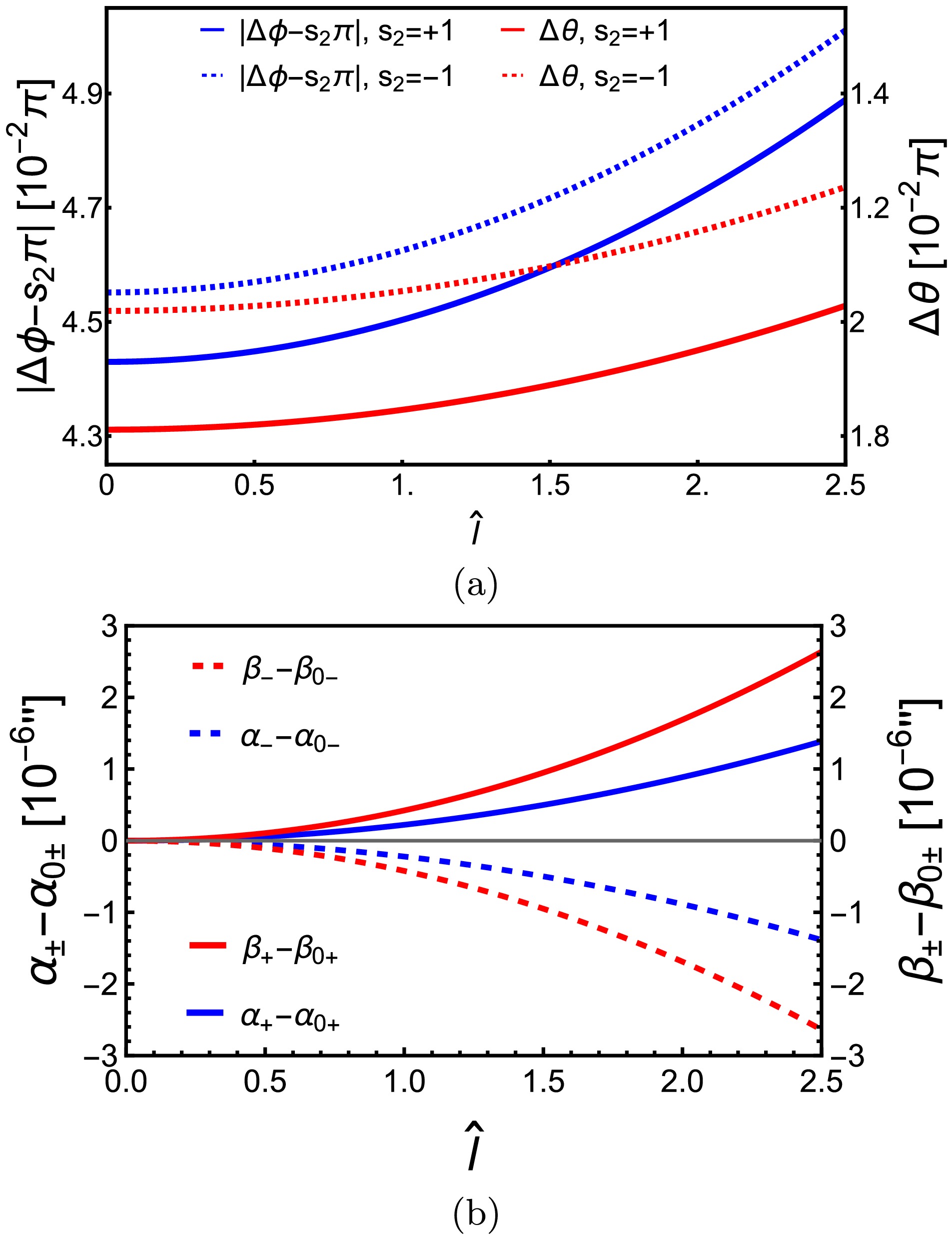

Figure 5.  (color online) Dependences of $ \Delta\phi $ and $ \Delta\theta $ (a) and α and β (b) on $ \hat{l} $ in RSV spacetime. In (a), $ r_s = r_d = 400M,\,\theta_m = \pi/5,\, $$ r_0 = 20M,\,\theta_s = \pi/4 $ are used to clearly show the effect. In (b), $ M = 4.1\times 10^6M_\odot,\,r_s = r_d = 8.34\; \mathrm{kpc},\, \delta \theta = 10^{-4\prime\prime},\,\delta \phi = 10^{-4\prime\prime},\,\theta_s = $$ \pi/6 $. In both plots, $ v = 1,\,\hat{a} = 1/2 $ are used.

After solving $ (r_0,\,\theta_m) $ and substituting into Eq. (49), we determine the apparent angles in the RSV spacetime to be

where $ \Theta_\pm $ is still given by Eq. (55), whereas its $ (L_\pm,\, K_\pm) $ depends on $ (r_{0\pm},\,\theta_{m\pm}) $ through Eqs. (22) and (23). The approximations of these apparent angles are

In Fig. 5 (b), we plot the dependences of the deflections $ (\Delta \phi_\mathrm{R},\, \Delta \theta_\mathrm{R}) $ and the apparent angles $ (\alpha_{\pm\mathrm{R}},\,\beta_{\pm\mathrm{R}}) $ on $ \hat{l} $. Unlike the effect of $ \hat{Q} $ in KN spacetime, here, $ \hat{l} $ increases $ r_{0\pm} $; consequently, the apparent angles of the images increase. The amount of reduction of either $ \alpha_{\pm R} $ or $ \beta_{\pm R} $ as $ \hat{l} $ increases to 2.5 is comparable to that for $ \hat{Q} $ in the KN case or $ \hat{b} $ in the KS case.

In this work, we have studied the off-equatorial deflections and GL of both null and timelike signals in general SAS spacetimes in the WDL, with the finite distance effect of the source and detector. We find that as long as the metric functions satisfy certain common separable variable conditions (10), which allows the existence of a GCC, the deflection angles in both the ϕ and θ directions can always be determined using the perturbative method. The results, as shown in Eqs. (41) and (44), are dual series of $ M/r_0 $ and $ r_0/r_{s,d} $, and can be directly used in a set of exact GL equations (46). These equations are then solved to determine the apparent angles of images in such spacetimes (49).

These results are then applied to the KN, KS, and RSV spacetimes to validate the correctness of the method and results and to determine the effect of the spacetime spin as well as that of the characteristic parameter (typically an effective charge) of these spacetimes. We find that both the spacetime spin and charge generally appear in the second order of both $ \Delta\phi $ and $ \Delta\theta $, whereas the non-equatorial effect appears from the very leading nontrivial order, as shown in Eqs. (52), (60) and (66).

For the image apparent angles, again both the spacetime spin and (effective) charge appear in the subleading, as manifested in Eqs. (56), (63), and (69). Therefore, these parameters are quite difficult to detect from the apparent angles in relativistic GL in the WDL.

To demonstrate the generality of our method, we supplement a few other spacetimes whose off-equatorial deflections can be determined using our method in Appendix B. We summarize the results computed in the main text and this appendix in Table 1 to clearly present the results and the effect of the main parameter(s) in the spacetime on the deflection and/or apparent angles.

Spacetime	Metric Eq.	Para.	Def. angle Eq.	Order	App. angle Eq.	Para. effect
Kerr-Newmann	(50)	Q	(52)	2	(56)	$ \searrow $
Kerr-Sen	(58)	b	(60)	2	(63)	$ \searrow $
Rotating Simpson-Visser	(64)	l	(66)	2	(69)	$ \nearrow $
Rotating Bardeen	(B1) with (B2)	g	(B7) with (B2)	3 or higher
Rotating Hayward	(B1) with (B3)	k	(B7) with (B3)	3 or higher
Rotating Ghosh	(B1) with (B4)	h	(B7) with (B4)	2
Rotating Tinchev	(B1) with (B5)	j	(B7) with (B5)	3 or higher

Table 1.  Spacetimes and their off equatorial deflections. From the second to last columns are the metric equation number, main parameter of the spacetime, deflection angles in that spacetime, lowest order in the deflection angle from which the main parameter appears, equation number of the image apparent angles for the spacetime studied in the main text, and effect of the parameter on the apparent angles, i.e., the monotonicity of the apparent angle as the parameter increases.

The results of this work can, in principle, be applied to any spacetime with a (non-spherical) axisymmetry. However, in the solar system, the only known object that can bend the light is the Sun, and yet its dimensionless spin parameter $ \hat{a} $ is only of order $ 10^{-20} $ [59]. Therefore, the effect of the spin or the off-equatorial plane effect in the deflection angle and/or apparent angle of images cannot be observed for the Sun in the foreseeable future. Instead, most spacetimes studied in this work are BH spacetimes. Therefore, the results are more applicable to more extreme rotating BHs, and particular examples are M87* [11] and Sgr A* [12], whose spin parameter $ \hat{a} $ can potentially reach a much larger order (roughly a fraction of one). We can also assume that such BHs carry extra parameters such as those appearing in the Kerr-Sen or rotating-Simpson-Visser spacetimes and attempt to use future observations to constrain the corresponding parameters.

A few potential extensions to this work that can be explored. The first is to study the magnification and time delays of the images in the off-equatorial GL. Ref. [33] shows that, for the Kerr spacetime, the spacetime spin might have a stronger effect on the time delay than on image locations. The second is that we might also attempt to study the off-equatorial deflection of charged particles in electromagnetic fields. However, the separation condition (10) must be re-investigated.

The authors are grateful for the helpful discussion with Tingyuan Jiang and Xiaoge Xu. The work of X. Ying is partially supported by the Undergraduate Training Programs for Innovation and Entrepreneurship of Wuhan University.

Here, we list some higher-order coefficients in the series appearing in the main text of the III. For Eq. (35), we present two more coefficients, which are also used in the computations in the main text:

where

The corresponding integral coefficients are

where

and

The second-order coefficient in Eq. (39) is

In addition to the spacetimes that we have discussed in detail in Sec. V, many spacetimes also satisfy the requirements of the separation of variables we establish in Sec. II A. Here, we briefly mention the off-equatorial deflections in these spacetimes.

The following line element describe a class of spacetimes satisfying these conditions

where

and $ a,\,m(r) $ are the spacetime spin and mass functions, respectively. This line element covers the Kerr spacetime when $ m(r) = M $ is a constant, the rotating Bardeen BH [43] when

the rotating Hayward BH [43] when

the rotating Ghosh BH [44] when

and the rotating Tinchev BH [45] when

Here, we have expanded $ m(r) $ into the following form:

and the coefficients $ m_n $ for each spacetime can be easily obtained from Eqs. (B2)－(B5). For the rotating Bardeen and Tinchev spacetimes, their characteristic parameter appears from the second order of the expansion, whereas the rotating Ghosh and Hayward ones appear from the first and third orders, respectively.

Using the line element (B1) and mass function (B6), we determine the deflection $ \Delta\theta $ and $ \Delta\phi $ as

where

and all $ m_i $ should be obtained from corresponding spacetime.

We also compute the deflection in the Konoplya-Zhidenko rotating non-Kerr spacetime whose metric is given by [42]

where

and η is the deformation parameter that describes the deviation from Kerr spacetime. However, we find that to order $ {\cal{O}}(M/r_0)^2 $, the parameter η does not appear in either $ \Delta\phi $ or $ \Delta\theta $. Therefore, the deflections to order $ {\cal{O}}(M/r_0)^2 $ in this spacetime is also given by Eq. (B7) with $ m_{n\geq 1} = 0 $.

For future reference, we also test the applicability of our methodology to SAS but non-asymptotically flat spacetimes, such as the KN-(anti)de Sitter spacetime described by [60]

where

and Kerr-Taub-NUT spacetime with metric [61]

where

We find that they also satisfy the separation requirements (10); therefore, the deflection of both null and timelike rays in the equatorial or off-equatorial plane in them can be treated using our method. Finally, for C-type metrics, which do not have the reflective symmetry about the equatorial plane, including the KN-(A)dS C-metric [62],

where

and its subcases with $ A\neq 0 $, we find that only for null but not the timelike rays, the separation requirements (10) can be satisfied. Therefore, the deflection can be studied using our approach. However, for these metrics, we will not list the formulas in the θ and ϕ directions until more valuable applications are determined.